
Chapter 2: Getting off the Ground with the First Deep Learning Model
Deep learning (DL) models have gained tremendous popularity in recent times and have caught the attention of data scientists in academia and industry alike. The reason behind their great success is their ability to solve the simplest yet oldest problem in computer science—computer vision. It had long been the dream of computer scientists to find an algorithm that would make machines see like humans do… or at least be able to recognize objects. DL models power not just object recognition but are used in everything, from predicting who is in an image, to natural language processing (NLP)—where they can be used for predicting and generating text and understanding speech—and even creating deepfakes, such as videos. At their core, all DL models are built using neural network (NN) algorithms; however, they are much more than just a NN. While NNs have been used since the 1950s, it's only in the last few years that DL has been able to make a big impact on the industry.
NNs were popularized in 1955 with a demonstration from International Business Machines Corporation (IBM) at the World Fair, where a machine made a prediction and the whole world saw the great potential of Artificial Intelligence (AI) to make machines learn anything and predict anything. That system was a perceptron-based network (a rudimentary cousin of what later became known as multilayer perceptrons (MLPs), which became the foundation for NNs and DL models).
With the success of NNs, many tried to use them for more advanced problems such as image recognition. The first such formal attempt at computer vision was made by a Massachusetts Institute of Technology (MIT) professor in 1965 (yes—machine learning (ML) was as big a thing back in the late 1950s and the early 1960s). He gave his students a summer assignment to find an algorithm for image recognition. No spoilers for guessing that despite their best efforts and unparalleled smartness, they failed to solve the problem that year. In fact, the problem of computer vision object recognition remained unsolved not just for years but for decades to come, a period popularly called the AI winter. The big breakthrough came in the mid-1990s with the invention of Convolutional Neural Networks (CNNs), a much-evolved form of NN. In 2012, when a more advanced version of a CNN trained at scale won the ImageNet competition and achieved accuracy rates as high as humans on the test set, it became the first choice for computer vision problems. After that, CNNs became not just the bedrock of image recognition problems but created a whole branch of ML called Deep Learning. Over the last few years, more advanced forms of CNNs have been devised, and new DL algorithms keep coming every single day that advance the state of the art (SOTA) and take human mastery of AI to new levels. In this chapter, we will examine the foundations of DL models, which are extremely important to understand, to make the best use of the latest algorithms. It is more than just a practice chapter, as MLPs and CNNs are still extremely useful for the majority of business applications. We will go through the following topics in this chapter:
- Getting started with NNs
- Building a Hello World MLP model
- Building our first DL model
- Working with a CNN model for image recognition
Technical requirements
The code for this chapter has been developed and tested on macOS with Anaconda or in Google Colaboratory (Google Colab) with Python 3.7. If you are using another environment, please make appropriate changes to your env variables.
In this chapter, we will primarily be using the following Python modules, mentioned with their versions:
- PyTorch Lightning (version: 1.5.2)
- Seaborn (version: 0.11.2)
- NumPy (version: 1.21.5)
- Torch (version: 1.10.0)
- pandas (version: 1.3.5)
!pip install torch==1.10.0 torchvision==0.11.1 torchtext==0.11.0 torchaudio==0.10.0 --quiet
!pip install pytorch-lightning==1.5.2 --quiet
In order to make sure that these modules work together and not go out of sync, we have used the specific version of torch, torchvision, torchtext, torchaudio with PyTorch Lightning 1.5.2. You can also use the latest version of PyTorch Lightning and torch compatible with each other. More details can be found on the GitHub link: https://github.com/PacktPublishing/Deep-Learning-with-PyTorch-Lightning
All the aforementioned packages are expected to be imported to Jupyter Notebook. You can refer to Chapter 1, PyTorch Lightning Adventure for guidance on importing packages.
You can find working examples of this chapter at the following GitHub link:
https://github.com/PacktPublishing/Deep-Learning-with-PyTorch-Lightning/tree/main/Chapter02
Here is the link to the Histopathologic Cancer Detection source dataset:
https://www.kaggle.com/c/histopathologic-cancer-detection
This dataset contains images of cancer tumors and images labeled with positive and negative identification. It consists of 327,680 color images, each with a size of 96x96 pixels (px), extracted from scans of lymph nodes. The data is provided under the Creative Commons (CC0) License. The link to the original dataset is https://github.com/basveeling/pcam; however, in this chapter, we will make use of the Kaggle source since it had been de-duplicated from the original set.
Getting started with Neural Networks
In this section, we will begin our journey by understanding the basics of Neural Networks.
Why Neural Networks?
Before we go deep into NNs, it is important to answer a simple question: Why do we even need a new classification algorithm when there are so many existing classification algorithms, such as decision trees? The simple answer is that there are some classification problems that decision trees would never be able to solve. As you might be aware, decision trees work by finding a set of objects in one class and then creating splits in the set to continue to create a pure class. This works well when there is a clear distinction between different classes in the dataset, but it fails when they are mixed. One such very basic problem that decision trees cannot ever solve is the XOR problem.
About the XOR operator
The XOR gate/operator is also known as exclusive OR. It is a digital logic in electronics. An XOR gate is a digital logic gate that produces a true output when it has dissimilar inputs. The following diagram shows the inputs and outputs (I/Os) generated by an XOR gate:
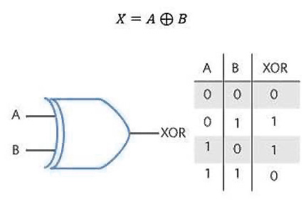
Figure 2.1 – XOR gate I/O truth table
In simple words, an XOR gate is a function that takes two inputs—for example, A and B—and generates a single output. From the preceding table, you can see that the XOR gate function gives us the following outputs:
- The output is 1 when the A and B inputs are different.
- The output is 0 when A and B are the same.
As you can see, if we want to build a decision-tree classifier, it will isolate 0 and 1 and will always give a prediction that is 50% wrong. There is no tree structure or logical boundary that can ever differentiate such a weird dataset. In other words, a decision-tree type of algorithm will never be able to solve this kind of classification problem. We need a fundamentally different approach to handle such a challenge.
In order to solve this problem, we need a fundamentally different kind of model that does not train on just input values but by conceptualizing I/O pairs and learning their relationship. That is the basis of the creation of NNs. It is not just another set of classifiers but a classifier that can solve problems others can't.
Neural Networks is an umbrella term for a range of classifiers under it, everything from a perceptron model to a DL model. One such basic yet incredibly powerful algorithm is MLP. The XOR problem mentioned here is one of the oldest yet very important problems to understand the origin story of NNs. You can think of XOR as a representation of all the problems that a decision-tree-type classifier can never solve since no visible boundary of classification is possible and we have to use a latent model to tackle it.
In this chapter, we will try to build our own simple MLP model to mimic the behavior of an XOR gate.
MLP architecture
Let's build an XOR NN architecture using the PyTorch Lightning framework. Our goal here is to build a simple MLP model, similar to the one shown in the following diagram:
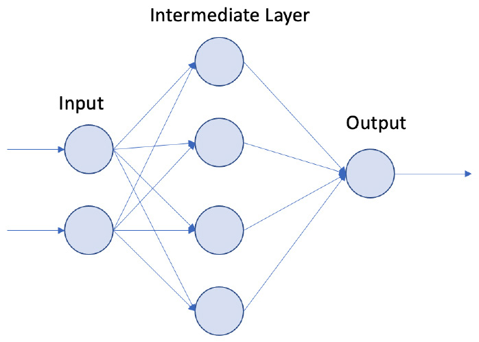
Figure 2.2 – MLP architecture
The preceding NN architecture diagram shows the following:
- An input layer, an intermediate layer, and an output layer.
- This architecture takes two inputs. This is where we pass the XOR inputs.
- The intermediate layer has four nodes.
- The final layer has a single node. This is where we expect the output of the XOR operation.
This NN that we will be building aims to mimic an XOR gate. Now, let's start coding our first PyTorch Lightning model!
Building a Hello World MLP model
Welcome to the world of PyTorch Lightning!
Finally, it's time for us to build our first model using PyTorch Lightning. In this section, we will build a simple MLP model to accomplish the XOR operator. This is like a Hello World introduction to the world of NNs as well as PyTorch Lightning. We will follow these steps to build our first XOR operator:
- Importing libraries
- Preparing the data
- Configuring the model
- Training the model
- Loading the model
- Making predictions
Importing libraries
We begin by first importing the necessary libraries and printing their package versions, as follows:
import pytorch_lightning as pl
import torch
from torch import nn, optim
from torch.autograd import Variable
import pytorch_lightning as pl
from pytorch_lightning.callbacks import ModelCheckpoint
from torch.utils.data import DataLoader
print("torch version:",torch.__version__)
print("pytorch ligthening version:",pl.__version__)
This code block should show the following output:
torch version: 1.10.0+cu111
pytorch ligthening version: 1.5.2
Once you have confirmed that you have the correct version, we are ready to start with the model.
Preparing the data
As you saw in Figure 2.1, an XOR gate takes two inputs and has four rows of data. In data science terms, we can call columns A and B our features and the Out column our target variable.
Before we start preparing our inputs and target data for XOR, it is important to understand that PyTorch Lightning accepts data loaders to train a model. In this section, we will build a simple data loader that has inputs and targets and will use it while training our model. We'll follow these next steps:
- It's time to build a truth table that matches the XOR gate. We will use the variables to create the dataset. The code for creating input features looks like this:
xor_inputs = [Variable(torch.Tensor([0, 0])),
Variable(torch.Tensor([0, 1])),
Variable(torch.Tensor([1, 0])),
Variable(torch.Tensor([1, 1]))]
Since PyTorch Lightning is built upon the PyTorch framework, all data that is being passed into the model must be in tensor form.
In the preceding code, we created four tensors, and each tensor had two values—that is, it had two features, A and B. We are ready with all the input features. A total of four rows are ready to be fed to our XOR model.
- Since the input features are ready, it's time to build our target variables, as shown in the following code snippet:
xor_targets = [Variable(torch.Tensor([0])),
Variable(torch.Tensor([1])),
Variable(torch.Tensor([1])),
Variable(torch.Tensor([0]))]
The preceding code for targets is similar to the input features' code. The only difference is that each target variable is a single value.
Inputs and targets will be ready in the final step of preparing our dataset. It's time to create a data loader. There are different ways in which we can create our dataset and pass it as a data loader to PyTorch Lightning. In the upcoming chapters, we will demonstrate different ways of using data loaders.
- Here, we will use the simplest way of building a dataset for our XOR model. The following code is used to do this:
xor_data = list(zip(xor_input, xor_target))
train_loader = DataLoader(xor_data, batch_size=1)
Data loaders in PyTorch Lightning look for two main things—the key and the value, which in our case are the features and target values. We are then using the DataLoader module from torch.utils.data to wrap the xor_data and create a Python iterable over the XOR data.
[(tensor([0., 0.]), tensor([0.])),
(tensor([0., 1.]), tensor([1.])),
(tensor([1., 0.]), tensor([1.])),
(tensor([1., 1.]), tensor([0.]))]
In the preceding code, we are creating a dataset that is a list of tuples, and each tuple has two values. The first values are the two features/inputs, and the second values are the target values for the given input.
Configuring the model
Finally, it's time to train our first PyTorch Lightning model. Models in PyTorch Lightning are built similarly to how they are built in PyTorch. One added advantage with PyTorch Lightning is that it will make your code more structured with its life cycle methods; most of the model training code is taken care of by the framework, which helps us avoid the boilerplate code.
Also, another great advantage of this framework is that we can easily scale DL models across multiple graphics processing units (GPUs) and tensor processing units (TPUs), which we will be using in the upcoming chapters.
Every model we build using PyTorch Lightning must be inherited from a class called LightningModule. This is a class that contains the boilerplate code, and this is also where we have Lightning life cycle methods. In simple terms, we can say that PyTorch LightningModule is the same as PyTorch nn.Module but with added life cycle methods and other operations. If we take a look at the source code, PyTorch LightningModule is inherited from PyTorch nn.Module. That means most of the functionality in PyTorch nn.Module is available in LightningModule as well.
Any PyTorch Lightning model needs at least two life cycle methods—one for the training loop to train the model (called training_step), and another to configure an optimizer for the model (called configure_optimizers). In addition to these two life cycle methods, we also use the forward method. This is where we take in the input data and pass it to the model.
Our XOR MLP model building follows this process, and we will go over each step in detail, as follows:
- Initializing the model
- Mapping inputs to the model
- Configuring the optimizer
- Setting up training parameters
Initializing the model
To initialize the model, follow these steps:
- Begin by creating a class called XOR that inherits from PyTorch LightningModule, which is shown in the following code snippet:
class XORModel(pl.LightningModule)
- We will start creating our layers. This can be initialized in the __init__ method, as demonstrated in the following code snippet:
def __init__(self):
super(XORModel,self).__init__()
self.input_layer = nn.Linear(2, 4)
self.output_layer = nn.Linear(4,1)
self.sigmoid = nn.Sigmoid()
self.loss = nn.MSELoss()
In the preceding code snippet, we performed the following actions:
- Setting up hidden layers, where the first layer takes in two inputs and returns four outputs, and that output becomes our intermediate layer. The intermediate layer merges with the single node, which becomes our output node.
- Initializing the activation function. Here, we are using the sigmoid function to build our XOR gate.
- Initializing the loss function. Here, we are using the mean squared error (MSE) loss function to build our XOR model.
Mapping inputs to the model
This is a simple step where we are using the forward method, which takes the inputs and generates the model's output. The following code snippet demonstrates the process:
def forward(self, input):
#print("INPUT:", input.shape)
x = self.input_layer(input)
#print("FIRST:", x.shape)
x = self.sigmoid(x)
#print("SECOND:", x.shape)
output = self.output_layer(x)
#print("THIRD:", output.shape)
return output
The forward method acts as a mapper or medium where data is passed between multiple layers and the activation function. In the preceding forward method, it's primarily doing the following operations:
- It takes the inputs for the XOR gate and passes them to our first input layer.
- Output generated from the first input layer is fed to the sigmoi activation function.
- Output from the sigmoid activation function is fed to the final layer, and the same output is being returned by the forward method.
- The commented-out print statements are for debugging and explanatory purposes. You can uncomment them and see how tensors are passed to the model and how model training works for deeper understanding.
Configuring the optimizer
All optimizers in PyTorch Lightning can be configured in a life cycle method called configure_optimizers. In this method, one or multiple optimizers can be configured. For this example, we can make use of single optimizers, and in future chapters, some models use multiple optimizers.
For our XOR model, we will use the Adam optimizer, and the following code snippet demonstrates our configure_optimizers life cycle methods:
def configure_optimizers(self):
params = self.parameters()
optimizer = optim.Adam(params=params, lr = 0.01)
return optimizer
All model parameters can be accessed by using the self object with the self.parameters() method. Here, we are creating an Adam optimizer that takes the model parameters with a learning rate (lr) of 0.01, and the same optimizer is being returned.
Important Note
To those who are not familiar with optimizers, it helps with the stochastic gradient descent (SGD) process and helps the model find global minima. You can learn more about how Adam works here: https://arxiv.org/abs/1412.6980.
Setting up training parameters
This is where all the model training occurs. Let's try to understand this method in detail. This is the code for training_step:
def training_step(self, batch, batch_idx):
xor_input, xor_target = batch
#print("XOR INPUT:", xor_input.shape)
#print("XOR TARGET:", xor_target.shape)
outputs = self(xor_input)
#print("XOR OUTPUT:", outputs.shape)
loss = self.loss(outputs, xor_target)
return loss
This training_step life cycle method takes the following two inputs:
- batch: Data that is being passed in the data loader is accessed in batches. This consists of two items: one is the input/features data, and the other item is targets.
- batch_idx: This is the index number or the sequence number for the batche of data.
In the preceding method, we are accessing our inputs and targets from the batch and then passing the inputs to the self method. When the input is passed to the self method, that indirectly invokes our forward method, which returns the XOR multilayer NN output. We are using the MSE loss function to calculate the loss and return the loss value for this method.
Important Note
Inputs passed to the self method indirectly invoke the forward method where the mapping of data happens between layers, and activation functions and output from the model are being generated.
Output from the training step is a single-loss value, whereas, in the upcoming chapter, we will cover different ways and tricks that will help us build and investigate our NN.
There are many other life cycle methods available in PyTorch Lightning. We will cover them in upcoming chapters, depending on the use case and scenario.
We have completed all the steps that are needed to build our first XOR MLP model. The complete code block for our XOR model looks like this:
class XORModel(pl.LightningModule):
def __init__(self):
super(XORModel,self).__init__()
self.input_layer = nn.Linear(2, 4)
self.output_layer = nn.Linear(4,1)
self.sigmoid = nn.Sigmoid()
self.loss = nn.MSELoss()
def forward(self, input):
#print("INPUT:", input.shape)
x = self.input_layer(input)
#print("FIRST:", x.shape)
x = self.sigmoid(x)
#print("SECOND:", x.shape)
output = self.output_layer(x)
#print("THIRD:", output.shape)
return output
def configure_optimizers(self):
params = self.parameters()
optimizer = optim.Adam(params=params, lr = 0.01)
return optimizer
def training_step(self, batch, batch_idx):
xor_input, xor_target = batch
#print("XOR INPUT:", xor_input.shape)
#print("XOR TARGET:", xor_target.shape)
outputs = self(xor_input)
#print("XOR OUTPUT:", outputs.shape)
loss = self.loss(outputs, xor_target)
return loss
To summarize, in the preceding code block, we have the following:
- The XOR model takes in XOR inputs of size 2.
- Data is being passed to the intermediate layer, which has four nodes and returns a single output.
- In this process, we are using sigmoid as our activation function, MSE as our loss function, and Adam as our optimizer.
If you observe, we have not set up any backpropagation, clearing gradients, or optimizer parameter updates and many other things are taken care of by the PyTorch Lightning framework.
Training the model
All models built in PyTorch Lightning can be trained using a Trainer class. Let's learn more about this class now.
The Trainer class is an abstraction of some key things, such as looping over the dataset, backpropagation, clearing gradients, and the optimizer step. All the boilerplate code from PyTorch is being taken by the Trainer class in PyTorch Lightning. Also, the Trainer class supports many other functionalities that help us to build our model easily, and some of those functionalities are various callbacks, model checkpoints, early stopping, dev runs for unit testing, support for GPUs and TPUs, loggers, logs, epochs, and many more. In various chapters in this book, we will try to cover most of the important features supported by the Trainer class.
The code for training our XOR model looks like this:
from pytorch_lightning.utilities.types import TRAIN_DATALOADERS
checkpoint_callback = ModelCheckpoint()
model = XORModel()
trainer = pl.Trainer(max_epochs=100, callbacks=[checkpoint_callback])
In the next step, we are creating a trainer object. We are running the model for a maximum of 100 epochs and also passing the model checkpoint as a callback. In the final step, once the model trainer is ready, we invoke the fit method by passing model and input data, which is shown in the following code snippet:
trainer.fit(model, train_dataloaders=train_loader)
In the preceding code snippet, we are training our model for 100 epochs and passing the data using the train_dataloaders argument.
We will get the following output after running the model for 100 epochs:

Figure 2.3 – Model output after 100 epochs
If we closely observe the progress of model training, at the end, we can see the loss value is being displayed. PyTorch Lightning supports a good and flexible way to configure values to be displayed on the progress bar, which we will cover in upcoming chapters.
To summarize this section, we have created an XOR model object and used the Trainer class to train the model for 100 epochs.
In PyTorch Lightning, one advantage we see is whenever we train a model multiple times, all the different model versions are saved to disk in a default folder called lightning_logs, and once all the models with different versions are made ready, we always have the opportunity to load the different model versions from the files and compare the results. For example, here, we have run the XOR model twice, and when we look at the lightning_logs folder, we can see two versions of the XOR model:
ls lightning_logs/
This should show the following output:
Figure 2.4 – List of files in the lightning_logs folder
Within these version subfolders, we have all the information about the model being trained and built, which can be easily loaded, and predictions can be performed. Files within these folders have some useful information, such as hyperparameters, which are saved as hparams.yaml, and we also have a subfolder called checkpoints. This is where our XOR model is stored in serialized form. Here is a screenshot of all the files within these version folders:
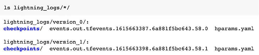
Figure 2.5 – List of subfolders and files within the lightning_logs folder
If you run multiple versions and want to load the latest version of the model from the preceding code snippet, the latest version of the model is stored in the version_1 folder. We can manually find the path to the latest version of the model or use model checkpoint callbacks.
Important Note
Please add ! for the shell commands run inside Colab.
Loading the model
Once we have built the model, the next step is to load that model. As mentioned in the preceding section, identifying the latest version of a model can be done using checkpoint_callback, created in the preceding step. Here, we have run two versions of the model to get the path of the latest version of the model, as shown in the following code snippet:
print(checkpoint_callback.best_model_path)
Here is the output of the preceding code, where the latest file path for the model is displayed. This is later used to load the model back from the checkpoint and make predictions:

Figure 2.6 – Output of the file path for the latest model version file
Loading the model from the checkpoint can easily be done using the load_from_checkpoint method from the model object by passing the model checkpoint path, which is shown in the following code snippet:
train_model = model.load_from_checkpoint(checkpoint_callback.best_model_path)
This preceding code will load the model from the checkpoint. In this step, we have built and trained the model for two different versions and loaded the latest model from the checkpoints.
Making predictions
Now that our model is ready, it's time to make some predictions. This process is demonstrated in the following code snippet:
test = torch.utils.data.DataLoader(xor_input, batch_size=1)
for val in xor_input:
_ = train_model(val)
print([int(val[0]),int(val[1])], int(_.round()))
This preceding code is an easy way to make predictions, iterating over our XOR dataset, passing the input values to the model, and making the prediction. This is the output of the preceding code snippet:

Figure 2.7 – XOR model output
From the preceding output, we can see that the input model had predicted the correct results. There are different ways and techniques to build a model, which we will cover in the upcoming chapters.
This may seem like a rather simple result but was a breakthrough in ML when it was first accomplished in the 1960s. We could make the machine learn behavior that does not follow a simple sequence of logical breakdowns such as decision trees and encapsulate the knowledge by simply observing I/O values. This core idea of observing I/O values and learning is exactly how an image recognition model using CNN works, whereby it matches an image representation with a label and learns to classify objects.
Building our first Deep Learning model
Now that we have built a basic NN, it's time to use our knowledge of creating an MLP to build a DL model. You will notice that the core framework will remain the same and is built upon the same foundation.
So, what makes it deep?
While the exact origins of who first used DL are often debated, a popular misconception is that DL just involves a really big NN model with hundreds or thousands of layers. While most DL models are big, it is important to understand that the real secret is a concept called backpropagation.
As we have seen, NNs such as MLPs have been around for a long time, and by themselves, they could solve previously unsolved classification problems such as XOR or give better predictions than traditional classifiers. However, they were still not accurate when dealing with large unstructured data such as images. In order to learn in high-dimensional spaces, a simple method called backpropagation is used, which gives feedback to the system. This feedback makes the model learn whether it is doing a good or bad job of predicting, and mistakes are penalized in every iteration of the model. Slowly, over lots of iterations using optimization methods, the system learns to minimize mistakes and achieves convergence. We converge by using the loss function for the feedback loop and continuously reduce the loss, thereby achieving the desired optimization. There are various loss functions available, with popular ones being log loss and cosine loss functions.
Backpropagation, when coupled with a massive amount of data and the computing power provided by the cloud, can do wonders, and that is what gave rise to the recent renaissance in ML. Since 2012, when a CNN architecture won the ImageNet competition with subsequent models achieving near-human accuracy, it has only got better. In this section, we will see how to build a CNN model. Let's start with an overview of a CNN architecture.
CNN architecture
As you all know, computers only understand the language of bits, which means they accept input in a numerical form. But how can you convert an image into a number? A CNN architecture is made of various layers that represent convolution. The simple objective of CNNs is to take a high-dimensional object, such as an image, and convert it into a lower-dimensional entity, such as a mathematical form of numbers, which is represented in matrix form (also known as a tensor).
Of course, a CNN does more than convert an image into a tensor. It also learns to recognize that object in an image using backpropagation and optimization methods. Once trained on the number of images, it can easily recognize unseen images accurately. The success of CNNs has been in their flexibility with regard to scale by simply adding more hardware and then giving a stellar performance in terms of accuracy the more they scale.
We will build a CNN model for the Histopathologic Cancer Detection dataset to identify metastatic cancer in small image patches taken from larger digital pathology scans. You can see an overview of this here:
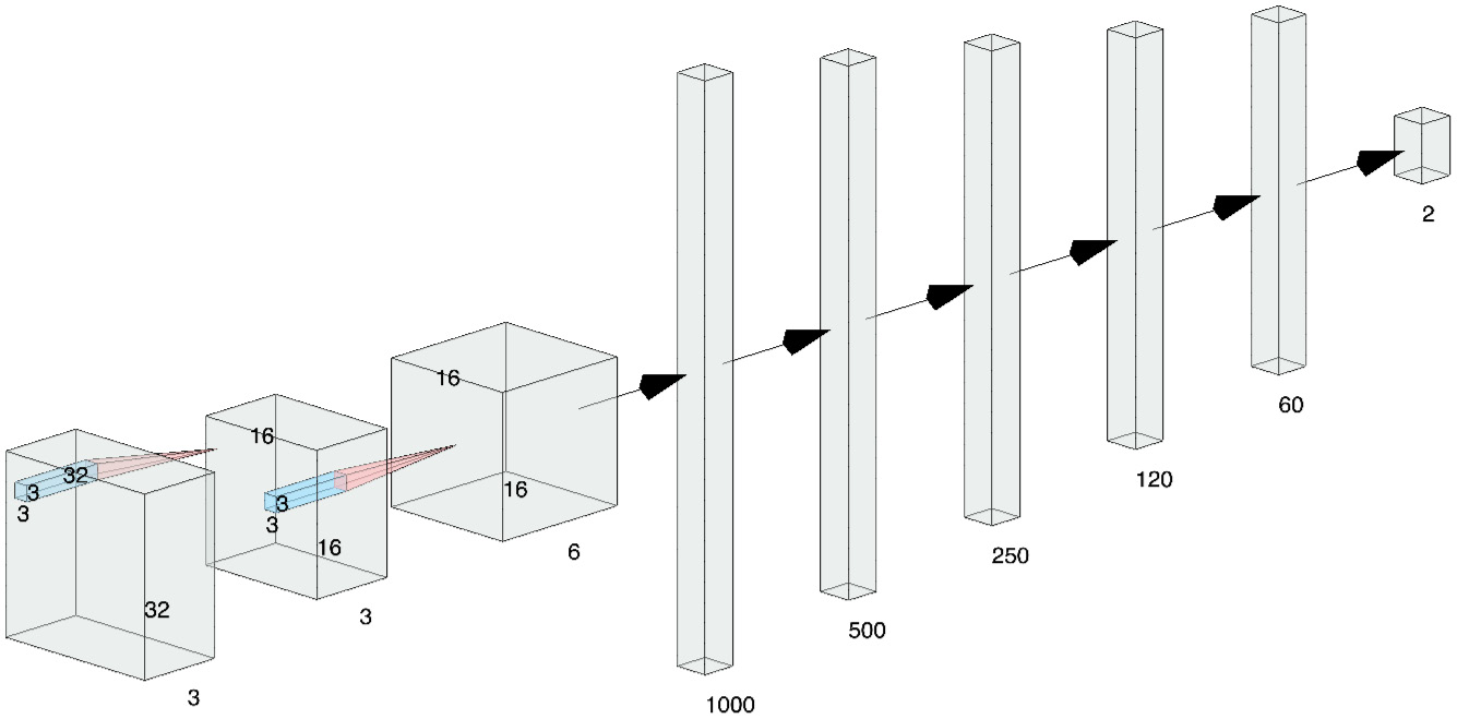
Figure 2.8 – CNN architecture for the Histopathologic Cancer Detection use case
We will use a simple 3 layer CNN architecture for our example.
The source image dataset starts with 96x96 images with three color channels. Cancer detection is based on the center 32x32px region if a patch contains at least one pixel of tumor tissue. Tumor tissue in the outer region of the patch does not influence the label. So, the original image is cropped to 32x32 size. We then do the following:
- We put it through the first convolution with a kernel size of 3 and a stride length of 1.
- The first convolution layer is followed by the MaxPool layer, where images are converted to lower-dimensional 16x16 objects.
- This is followed by another convolutional layer with six channels. This convolutional layer is followed by five fully connected layers of feature-length 1,000, 500, 250, 120, and 60 to finally get a SoftMax layer that gives the final predictions.
We will be using ReLU as our activation function, Adam as our optimizer, and Cross-Entropy as our loss function for training this model.
Building a CNN model for image recognition
PyTorch Lightning is a versatile framework, which makes training and scaling DL models easy by focusing on building models than writing complex programs. PyTorch Lightning is bundled with many useful features and options for building DL models. Since it is hard to cover all the topics in a single chapter, we will keep exploring different features of PyTorch Lightning in every chapter.
Here are the steps for building an image classifier using a CNN:
- Importing the packages
- Collecting the data
- Preparing the data
- Building the model
- Training the model
- Evaluating the accuracy of the model
Importing the packages
We will get started using the following steps:
- First things first—install and load the necessary packages, as follows:
!pip install torch==1.10.0 torchvision==0.11.1 torchtext==0.11.0 torchaudio==0.10.0 --quiet
!pip install pytorch-lightning==1.5.2 --quiet
!pip install opendatasets --upgrade --quiet
- Then, please import the following packages before getting started:
import os
import shutil
import opendatasets as od
import pandas as pd
import numpy as np
from PIL import Image
from sklearn.metrics import confusion_matrix
from sklearn.model_selection import train_test_split
import matplotlib.pyplot as plt
import torch
from torch import nn, optim
from torch.utils.data import DataLoader, Dataset
from torch.utils.data.sampler import SubsetRandomSampler
from torchvision.datasets import ImageFolder
import torchvision.transforms as T
from torchvision.utils import make_grid
from torchmetrics.functional import accuracy
import pytorch_lightning as pl
- The following commands should allow us to get started:
print("pandas version:",pd.__version__)
print("numpy version:",np.__version__)
#print("seaborn version:",sns.__version__)
print("torch version:",torch.__version__)
print("pytorch ligthening version:",pl.__version__)
- Executing the following code will ensure that you have the correct versions as well:
pandas version: 1.3.5
numpy version: 1.21.5
torch version: 1.10.0+cu111
pytorch ligthening version: 1.5.2
We can now start building our model by first collecting our data.
Collecting the data
We will now make use of Google Drive to store the dataset as well as to later save the checkpoint. You would need to mount the drive as shown in the GitHub notebook before you complete this step and provide the path where the dataset is downloaded. You can refer to Chapter 10, Scaling and Managing Training, on using cloud storage with Colab notebooks.
Firstly, we need to download the dataset from Kaggle, as shown here:
dataset_url = 'https://www.kaggle.com/c/histopathologic-cancer-detection'
od.download(dataset_url)
Here, we are downloading the PCam dataset from Kaggle using the credentials. You will be prompted to enter your username and key, which can be obtained from Kaggle's website:
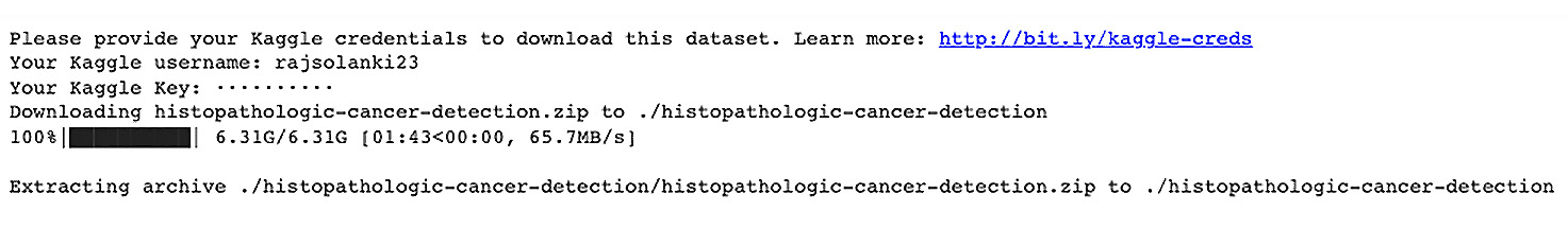
Figure 2.9 – Downloading the dataset from Kaggle
Important Note
To create an application programming interface (API) key in Kaggle, go to kaggle.com/ and open your Account settings page. Next scroll down to the API section and click on the Create New API Token button. This will download a file called Kaggle.json on your computer from which you can get your username and the key or else upload the Kaggle.json file directly to your Google Colab folder to use it in the notebook.
There is a separate file called train_labels.csv that contains image identifiers (IDs) and their respective label/ground truth. So, we will read this file into a pandas DataFrame, as shown here:
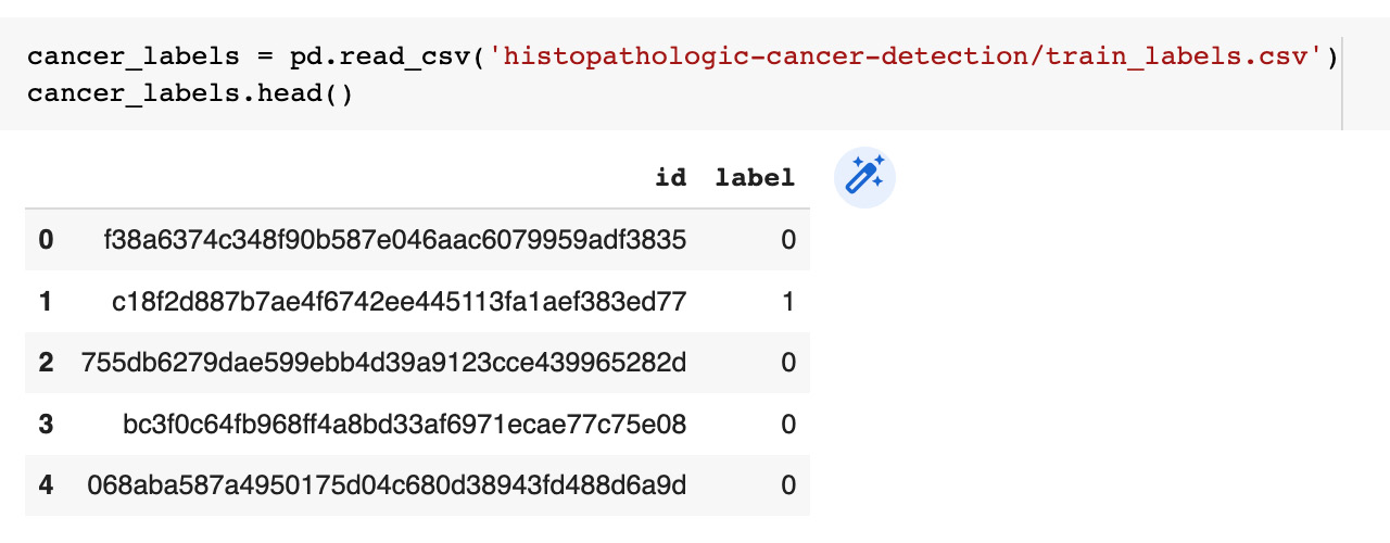
Figure 2.10 – Reading the labels file
You can observe from the output shown in Figure 2.11 that there are two labels for the images, 0 and 1, so it is a binary classification task.
Preparing the data
The data preparation process will itself consist of multiple steps, as follows:
- Downsampling the data
- Loading the dataset
- Augmenting the dataset
The PatchCamelyon (PCam) dataset for histopathological cancer detection consists of 327,680 color images extracted from histopathologic scans of lymph nodes. Each image is annotated with a binary label (positive or negative) indicating the presence of metastatic tissue. It has the following subfolders:
histopathologic-cancer-detection/train
histopathologic-cancer-detection/test
The first path has around 220,000 images of histopathologic scans, while the second path has around 57,000 images of histopathologic scans. The train_labels.csv file shown in the following snippet contains the ground truth for the images in the train folder:
histopathologic-cancer-detection/train_labels.csv
Here are some example images of histopathological scans:
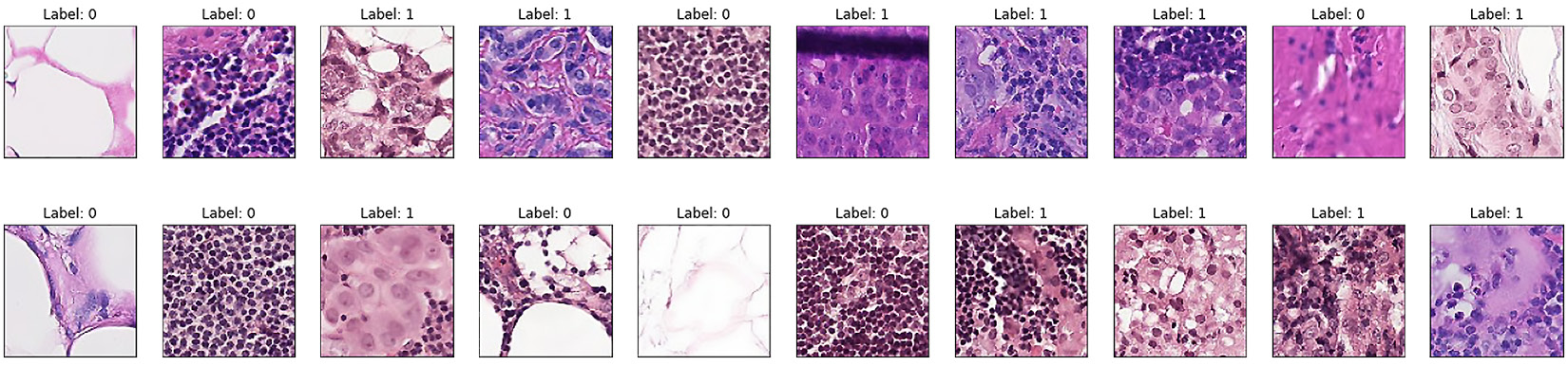
Figure 2.11 – Sample images of histopathological scans
Downsampling the dataset
A positive label indicates that the center 32x32 px region of a patch contains at least one px of tumor tissue. There are 130,908 normal cases (0) and 89,117 abnormal (or cancerous) tissue images (1). This is a huge dataset that will require a lot of time and compute resources to train on a full dataset, thus for the purpose of learning our first image classification model, we will downsample the 220,000 images in the train folder to 10,000 images and then split them into training and testing datasets, as shown in the following code block:
np.random.seed(0)
train_imgs_orig = os.listdir("histopathologic-cancer-detection/train")
selected_image_list = []
for img in np.random.choice(train_imgs_orig, 10000):
selected_image_list.append(img)
len(selected_image_list)
In the preceding code snippet, we are first setting the seed to make the results reproducible (feel free to use any number in the random.seed() method). Then, we are randomly selecting 10,000 images names (or IDs) from the train folder and storing them in selected_image_list. Once the 10,000 images are selected, we will split the data into train and test data, as shown here:
np.random.seed(0)
np.random.shuffle(selected_image_list)
cancer_train_idx = selected_image_list[:8000]
cancer_test_idx = selected_image_list[8000:]
print("Number of images in the downsampled training dataset: ", len(cancer_train_idx))
print("Number of images in the downsampled testing dataset: ", len(cancer_test_idx))
In the preceding code snippet, we are again setting the seed to make the results reproducible. Then, we are shuffling the image list and selecting 8000 image names (or IDs) that are stored in cancer_train_idx and the remaining 2000 image names in cancer_test_idx. The output is shown here:
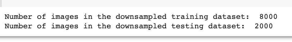
Figure 2.12 – Number of train and test images
Once the train and test image names are stored in cancer_train_idx and cancer_test_idx respectively, we need to store those 8,000 and 2,000 images on persistent storage on Google Drive so that we don't have to redo all of this during the model improvement exercise or when debugging the code. You can mount the persistent storage using the following code:
from google.colab import drive
drive.mount('/content/gdrive')
This results in the following output:
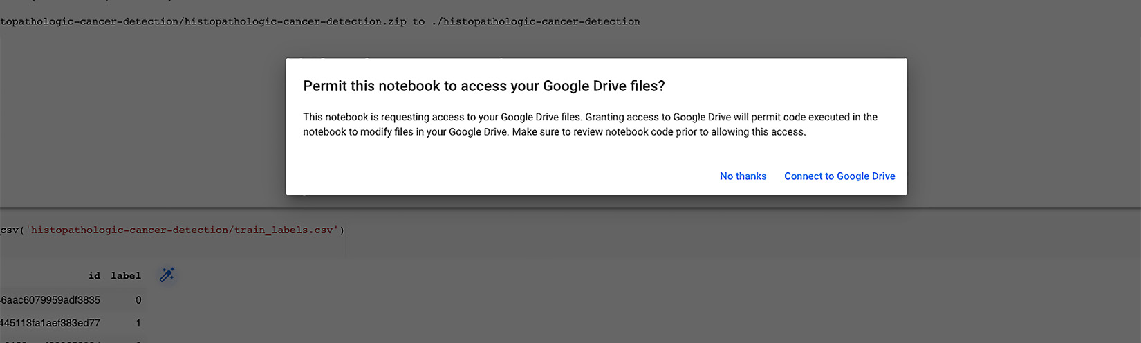
Figure 2.13 – Allowing access to Google Drive
You will be prompted to allow access to your drive; once you accept it, your drive will be mounted and you can access any of the data stored on persistent storage even after the session expires, and you can resume your work without having to download, downsample, and split the data again. The code for storing the images on persistent storage is shown here:
os.mkdir('/content/gdrive/My Drive/Colab Notebooks/histopathologic-cancer-detection/train_dataset/')
for fname in cancer_train_idx:
src = os.path.join('histopathologic-cancer-detection/train', fname)
dst = os.path.join('/content/gdrive/My Drive/Colab Notebooks/histopathologic-cancer-detection/train_dataset/', fname)
shutil.copyfile(src, dst)
In the preceding code snippet, we are first creating a folder called train_dataset on the following path:
content/gdrive/My Drive/Colab Notebooks/histopathologic-cancer-detection/
Then, we are looping over cancer_train_idx to get image names for the training data and copying all the files from local storage in the machine allotted to us at the time we created a notebook to persistent storage on our Google Drive using the shutils Python module. We will also repeat this exercise for the test dataset. The code is illustrated in the following snippet:
os.mkdir('/content/histopathologic-cancer-detection/test_dataset/')
for fname in test_idx:
src = os.path.join('histopathologic-cancer-detection/train', fname)
dst = os.path.join('/content/histopathologic-cancer-detection/test_dataset/', fname)
shutil.copyfile(src, dst)
print('No. of images in downsampled testing dataset: ', len(os.listdir("/content/histopathologic-cancer-detection/test_dataset/")))
As shown in the preceding code snippet, we are saving the training and testing dataset in the persistent storage on Google Drive for further use and to help in tuning the image classification model.
The labels for the images that were selected in the downsampled data will be extracted in a list that will be used for training and evaluating the image classification model, as shown here:
selected_image_labels = pd.DataFrame()
id_list = []
label_list = []
for img in selected_image_list:
label_tuple = df_labels.loc[df_labels['id'] == img.split('.')[0]]
id_list.append(label_tuple['id'].values[0])
label_list.append(label_tuple['label'].values[0])
Loading the dataset
PyTorch Lightning expects data to be in folders with the classes. So, we cannot use the DataLoader module directly when all train/test images are in one folder without subfolders. Therefore, we will write our custom class for loading the data, as follows:
class LoadCancerDataset(Dataset):
def __init__(self, data_folder,
transform = T.Compose([T.CenterCrop(32),T.ToTensor()]), dict_labels={}):
self.data_folder = data_folder
self.list_image_files = [s for s in os.listdir(data_folder)]
self.transform = transform
self.dict_labels = dict_labels
self.labels = [dict_labels[i.split('.')[0]] for i in self.list_image_files]
def __len__(self):
return len(self.list_image_files)
def __getitem__(self, idx):
img_name = os.path.join(self.data_folder, self.list_image_files[idx])
image = Image.open(img_name)
image = self.transform(image)
img_name_short = self.list_image_files[idx].split('.')[0]
label = self.dict_labels[img_name_short]
return image, label
In the preceding code block, we have defined a custom data loader.
The custom class defined earlier inherits from the torch.utils.data.Dataset module. The LoadCancerDataset custom class is initialized in the __init__ method and accepts three arguments: the path to the data folder, the transformer with a default value of cropping the image to size 32 and transforming it to a tensor, and a dictionary with the labels and IDs of the dataset.
The LoadCancerDataset class reads all the images in the folder and extracts the image name from the filename, which is also the ID for the images. This image name is then matched with the label in the dictionary with the labels and IDs.
The LoadCancerDataset class returns the images and their labels, which can then be used in the DataLoader module of the torch.utils.data library as it can now read the images with their corresponding label.
Now we need to create a dictionary with labels and IDs that will be used in our LoadCancerDataset class:
img_class_dict = {k:v for k, v in zip(selected_image_labels.id, selected_image_labels.label)}
The preceding code extracts the ID and labels from the selected_image_labels data frame and stores them in the img_class_dict dictionary.
Augmenting the dataset
Now that we have loaded the data, we will start the process of data preprocessing by augmenting the images, as follows:
data_T_train = T.Compose([
T.CenterCrop(32),
T.RandomHorizontalFlip(),
T.RandomVerticalFlip(),
T.ToTensor(),
])
data_T_test = T.Compose([
T.CenterCrop(32),
T.ToTensor(),
])
In the preceding code block, we have used transformations to crop the image to 32x32 by using Torchvision's built-in libraries. We then also augmented the data by flipping it horizontally and vertically, thereby creating two additional copies from the original image.
Now, we will call our LoadCancerDataset custom class with the path to the data folder, transformer, and the image label dictionary to convert it to the format accepted by the torch.utils.data.DataLoader module. The code to achieve this is illustrated in the following snippet:
train_set = LoadCancerDataset(data_folder='/content/gdrive/My Drive/Colab Notebooks/histopathologic-cancer-detection/train_dataset/',
# datatype='train',
transform=data_T_train, dict_labels=img_label_dict)
This will be repeated for the test data as well, and then, in the final step, we will create train_dataloader and test_dataloader data loaders using the output from our LoadCancerDataset custom class by leveraging the DataLoader module from the torch.utils.data library. The code to do so is illustrated in the following snippet:
batch_size = 256
train_dataloader = DataLoader(dataset, batch_size, num_workers=2, pin_memory=True, shuffle=True)
test_dataloader = DataLoader(test_set, batch_size, num_workers=2, pin_memory=True)
In the preceding code snippet, we have the following:
- We started with the original data without the subfolders as expected by the PyTorch Lightning module. The data was downsampled and saved on Google Drive's persistent storage.
- Using the LoadCancerDataset custom class, we created two datasets train_set and test_set, by reading images and their labels.
- In the process of creating datasets, we also used the Torchvision transform module to crop the images to the center, that is, converting images to the square of 32 x 32 px and also converting images to tensors.
- In the final step, the two train_set and test_set datasets that were created are used to create two train_dataloader and test_dataloader data loaders for them.
At this point, we are ready with our train_dataloader data loader with around 8,000 images, and test_dataloader with around 2,000 images. All the images are of size 32 x 32, converted to tensor form, and served in batches of 256 images. We will use the train data loader to train our model and the test data loader to measure our model's accuracy.
Building the model
To build our CNN image classifier, let's divide the process into multiple steps, as follows:
- Initializing the model
- Configuring the optimizer
- Configuring training and testing
Initializing the model
Similar to the XOR model, we will begin by creating a class called CNNImageClassifier that inherits from the PyTorch LightningModule class, as shown in the following code snippet:
class CNNImageClassifier(pl.LightningModule)
Important Note
Every model that is built in a PyTorch Lightning (PL) must inherit from PyTorch LightningModule, as we will see throughout this book.
- Let's start by setting up our CNN ImageClassifier class. This can be initialized in the __init__ method, as shown in the following code snippet. We will break this method into chunks to make it easier for you to understand:
def __init__(self, learning_rate = 0.001):
super().__init__()
self.learning_rate = learning_rate
In the preceding code snippet, the CNN ImageClassifier class accepts a single parameter—the learning rate, with a default value of 0.001.
Important Note
The learning rate determines "how well" and "how fast" an ML algorithm "learns". This job of optimizing the learning path is performed by an optimizer (Adam, in this case). There is often a trade-off between accuracy and speed. A very low learning rate may learn well but it may take too long and get stuck in local minima. A very high learning rate may reduce loss initially but then never converge. In reality, this is a hyperparameter setting that needs to be tuned for each model.
- Next, we will build two convolution layers. Here is the code for building two convolution layers, along with max pooling and activation functions:
#Input size (256, 3, 32, 32)
self.conv_layer1 = nn.Conv2d(in_channels=3,out_channels=3,kernel_size=3,stride=1,padding=1)
#output_shape: (256, 3, 32, 32)
self.relu1=nn.ReLU()
#output_shape: (256, 3, 32, 32)
self.pool=nn.MaxPool2d(kernel_size=2)
#output_shape: (256, 3, 16, 16)
self.conv_layer2 = nn.Conv2d(in_channels=3,out_channels=6,kernel_size=3,stride=1,padding=1)
#output_shape: (256, 3, 16, 16)
self.relu2=nn.ReLU()
#output_shape: (256, 6, 16, 16)
In the preceding code snippet, we primarily built two convolutional layers—conv_layer1 and conv_layer2. Our images from the data loaders are in batches of 256, which are colored, and thus it has three input channels (red-green-blue, or RGB) with a size of 32 x 32.
Our first convolution layer, called conv_layer1, takes an input of size (256, 3, 32, 32), which is 256 images with three channels (RGB) of size 32 in width and height. If we look at conv_layer1, it is a two-dimensional (2D) CNN that takes three input channels and outputs three channels, with a kernel size of 3 and a stride and padding of 1 px. We also initialized max pooling with a kernel size of 2.
The second convolution layer, conv_layer2, takes three input channels as input and outputs six channels with a kernel size of 3 and a stride and padding of 1. Here, we are using two ReLU activation functions initialized in variables as relu1 and relu2. In the next section, we will cover how we pass data over these layers.
- In the following snippet, we will build six fully connected linear layers followed by a loss function. The code for six fully linear layers along with the loss function looks like this:
self.fully_connected_1 =nn.Linear(in_features=16 * 16 * 6,out_features=1000)
self.fully_connected_2 =nn.Linear(in_features=1000,out_features=500)
self.fully_connected_3 =nn.Linear(in_features=500,out_features=250)
self.fully_connected_4 =nn.Linear(in_features=250,out_features=120)
self.fully_connected_5 =nn.Linear(in_features=120,out_features=60)
self.fully_connected_6 =nn.Linear(in_features=60,out_features=2)
self.loss = nn.CrossEntropyLoss()
In the preceding code snippet, we had six fully connected linear layers, as follows:
- The first linear layer—that is, self.fully_connected_1—takes the input, which is the output generated from conv_layer2, and this self.fully_connected_1 layer outputs 1,000 nodes.
- The second linear layer—that is, self.fully_connected_2—takes the output from the first linear layer and outputs 500 nodes.
- Similarly, the third linear layer—that is, self.fully_connected_3—takes the output from the second linear layer and outputs 250 nodes.
- Then, the fourth linear layer—that is, self.fully_connected_4—takes the output from the third linear layer and outputs 120 nodes.
- Subsequently, the fifth linear layer—that is, self.fully_connected_5—takes the output from the fourth linear layer and outputs 60 nodes.
- The final layer—that is, self.fully_connected_6—takes the output from the fifth layer and outputs two nodes.
Since this is a binary classification, the output of this NN architecture should be the probability for the two classes. Finally, we will initialize the loss function, which is cross-entropy loss.
Important Note – Loss Function
A loss function is a method by which we measure how well our model is converging. As the model is trained through various epochs, the loss should tend toward zero (though it may not or never should reach zero). The cross-entropy loss function is one of the many loss functions available in DL models and is a good choice for image recognition models. You can read about the theory of the cross-entropy loss function here: https://en.wikipedia.org/wiki/Cross_entropy.
- Our NN architecture is defined as a combination of CNN and fully connected linear networks, so it's time to pass in the data from the different layers and the activation functions. We will do this with the help of the forward method:
def forward(self, input):
output=self.conv_layer1(input)
output=self.relu1(output)
output=self.pool(output)
output=self.conv_layer2(output)
output=self.relu2(output)
output=output.view(-1, 6*16*16)
output = self.fully_connected_1(output)
output = self.fully_connected_2(output)
output = self.fully_connected_3(output)
output = self.fully_connected_4(output)
output = self.fully_connected_5(output)
output = self.fully_connected_6(output)
return output
In the preceding code block, we have used the forward method. To summarize, in the forward method, the input image data is first passed over the two convolution layers, and then the output from the convolution layers is passed over six fully connected layers. Finally, the output is returned. Let's understand this step by step, as follows:
- The data is passed to our first convolution layer (conv_layer1). The output from conv_layer1 is passed to the ReLU activation function, and the output from ReLU is passed to the max-pooling layer.
- Once the input data is being processed by the first convolution layer, the activation function undergoes the max-pooling layer.
- Then, the output is passed to our second convolution layer (conv_layer2), and the output from the second convolution layer is passed to our second ReLU activation function.
- Data is passed through the convolution layer, and the output from these layers, is multidimensional. To pass the output to our linear layers, it is converted to a single-dimensional form, which can be achieved using the tensor view method.
- Once the data is ready in single-dimensional form, it is passed over six fully connected layers and the final output is returned.
Important Note
Hyperparameters can be saved using a method called save_hyperparameters(). This technique will be covered in upcoming chapters.
Configuring the optimizer
We have seen earlier that we will be using the Adam optimizer in this architecture to minimize our loss and converge the model. In order to do so, we need to configure optimizers that are available as one of the life cycle methods in PyTorch Lightning work.
The code for the configure_optimizers life cycle method for our CNNImageClassifier model looks like this:
def configure_optimizers(self):
params = self.parameters()
optimizer = optim.Adam(params=params, lr = self.learning_rate)
return optimizer
In the preceding code snippet, we are using the Adam optimizer with a learning rate that has been initialized in the __init__() method, and we then return the optimizer from this method.
The configure_optimizers method can return up to six different outputs. As in the preceding example, it can also return a single list/tuple object. With multiple optimizers, it can return two separate lists: one for the optimizers, and a second consisting of the learning-rate scheduler.
Important Note
configure_optimizers can return six different outputs. We will not cover all the cases in this book, but some of them have been used in our upcoming chapters on advanced topics.
For example, when we build some complex NN architectures, such as generative adversarial network (GAN) models, there may be a need for multiple optimizers, and in some cases, we may need a learning rate scheduler along with optimizers. This can be addressed by configuring optimizers in a life cycle method.
Configuring the training and testing steps
In the XOR model we have covered, one of the life cycle methods that helps us to train our model on the training dataset is training_step. Similarly, if we want to test our model on the test dataset, we have a life cycle method called test_step.
For our CNNImageClassifier model, we have used the life cycle methods for training and also for testing.
The code for the PyTorch Lightning training_step life cycle method looks like this:
def training_step(self, batch, batch_idx):
inputs, targets = batch
outputs = self(inputs)
train_accuracy = accuracy(outputs, targets)
loss = self.loss(outputs, targets)
self.log('train_accuracy', train_accuracy, prog_bar=True)
self.log('train_loss', loss)
return {"loss":loss, "train_accuracy": train_accuracy }
In the preceding code block, we have the following:
- In the training_step life cycle method, batches of data are accessed a input parameters and input data is passed to the model.
- We then calculate loss using the self.loss function.
- The next step is to calculate accuracy. For this, we use a utility function called accuracy() from the torchmetrics.functional module. This method takes in the actual targets and the predicted output of the model as input and calculates the accuracy. The complete code for the accuracy method is available using the GitHub link for the book.
We will perform some additional steps here that were not done in our XOR model. We will use the self.log function and log some of the additional metrics. The following code will help us log our train_accuracy and also train_loss metrics:
self.log('train_accuracy', train_accuracy, prog_bar=True)
self.log('train_loss', loss)
In the preceding code snippet, the self.log method accepts the key/name of the metrics as the first parameter, the second parameter is the value for the metric, and the third parameter that we passed is prog_bar by default, which is always set to false.
We are logging accuracy and loss for our train dataset. These logged values can be later used for plotting our charts or for further investigation and will help us to tune the model. By setting the prog_bar parameter to true, it will display the train_accuracy metric on the progress bar for each epoch while training the model.
This life cycle method can return a dictionary as output with loss and test accuracy.
The code for the test_step life cycle method looks like this:
def test_step(self, batch, batch_idx):
inputs, targets = batch
outputs = self.forward(inputs)
test_accuracy = self.binary_accuracy(outputs,targets)
loss = self.loss(outputs, targets)
self.log('test_accuracy', test_accuracy)
return {"test_loss":loss, "test_accuracy": test_accuracy }
The code for the test_step life cycle method is similar to the training_step life cycle method; the only difference is that the data being passed to this method is the test dataset. We will see how this method is being triggered in the next section of this chapter.
In this model, we will focus on logging some additional metrics and also display some metrics on the progress bar while training the model.
Training the model
One of the key features of the PyTorch Lightning framework is the simplicity with which we can train the model. The trainer class comes in handy for doing training along with easy-to-use options such as picking the hardware (cpu/gpu/tpu), controlling training epochs, and all other nice things.
In PyTorch Lightning, to train the model, we first initialize the trainer class and then invoke the fit method to actually train the model. The code snippet for training our CNNImageClassifier model is shown here:
model = CNNImageClassifier()
trainer = pl.Trainer(max_epochs=500, progress_bar_refresh_rate=50, gpus=-1)
trainer.fit(model, train_dataloader=train_dataloader)
In the preceding code snippet, we started by initializing our CNNImageClassifier model with a default learning rate of 0.001.
Then, we initialized the trainer class object from the PyTorch Lightning framework with 500 epochs, making use of all the available GPUs and setting the progress bar rate to 50.
We ran our model, which is making use of the GPU for computation and running for a total of 500 epochs, which reduces the training time to 20 minutes. The results for both the 100-epochs run and 500-epochs run are captured.
Whenever we train any PyTorch Lightning model, mainly on Jupyter Notebook, the progress of training for each epoch is visualized in a progress bar. This parameter helps us to control the speed to update this progress bar. The fit method is where we are passing our model and the train data loader, which we created earlier in the previous section. The data from the train data loader is accessed in batches in our training_step life cycle method, and that is where we train and calculate the loss. The process is illustrated in the following screenshot:
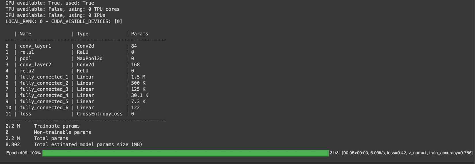
Figure 2.14 – Training image classifier for 500 epochs
The preceding screenshot shows the metrics used for training. You can see in the result set that two convolution layers followed by six fully connected layers' parameters are listed, and a cross-entropy loss is calculated.
In training_step, we logged the train_accuracy metric and set the prog_bar value to true. This enables the train_accuracy metric to be displayed on the progress bar for every epoch, as shown in the preceding results.
At this point, we have trained our model on the training dataset for 100 epochs and, as per the train_accuracy metric displayed on the progress bar, the training accuracy is 76%.
While the model is performing relatively well on the training dataset, it is important to check how well our model performs on the test dataset. The performance on the test dataset is an indication of how reliable the model will be in detecting unseen or new cancer-tissue images.
Evaluating the accuracy of the model
To calculate the accuracy of the model, we need to pass test data into our test data loader and check the accuracy on the test dataset. The following code snippet shows how to do this:
trainer.test(test_dataloaders=test_dataloader)
In the preceding code snippet, we are calling the test method from the trainer object and passing in the test data loader. When we do this, PyTorch Lightning internally invokes our test_step life cycle method and passes in the data in batches.
The output of the preceding code gives us the test accuracy, as shown here:
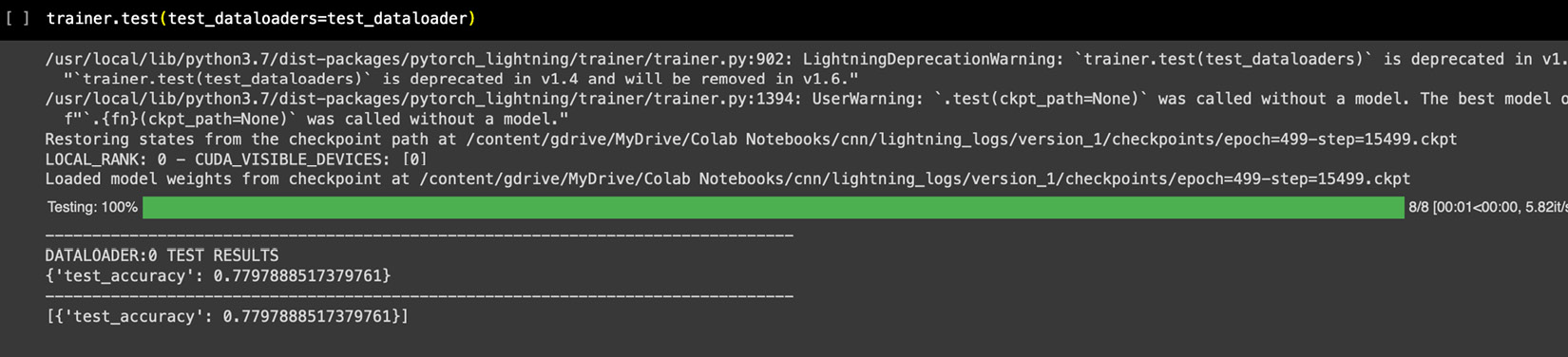
Figure 2.15 – Output of the test method
From the preceding output, our ImageClassifier model gives us an accuracy of 78% on our test dataset. This means that our model is performing really well on the test dataset as well, and we can use this model to correctly diagnose 8 of 10 cases of cancer tissues based on their image scans.
You may be wondering how this model actually gets deployed so that we can pass an unseen image scan of tissue and a user gets a prediction as to whether that image is cancerous or not. That process is called "scoring a model" and needs the deployment of an ML model—we will cover that in Chapter 9, Deploying and Scoring Models.
Important Note – Overfitting
You may have noticed that our model has really good accuracy on the train dataset as well as quite a good accuracy on the test dataset. This is a sign of a well-trained model. If you observe that accuracy between train and test scores is widely off (such as very good accuracy on the train set but very poor accuracy on the test set) then such behavior is normally known as overfitting. This typically happens when the model memorizes a training set while not generalizing on an unseen dataset. There are various methods to make models perform better on a test dataset, and such methods are called regularization methods. Batch normalization, dropout, and so on can be useful in regularizing the model. You can try them, and you will see improvement in test accuracy. We will also use them in future chapters.
Model improvement exercises
So, our first DL model is ready and is performing really well, considering the fact that we have trained it on just a sample set of a larger set. It was also relatively smooth to create this model using PyTorch Lightning, which made coding for CNN so straightforward. You can further try some of the following exercises to make this even better:
- Try running the model for more epochs and see how the accuracy improves. We have downsampled 10,000 images from the larger set. A DL model typically performs much better with larger datasets. You can try running it over a larger set and see the difference in accuracy (more GPU power may be needed).
- Try adjusting the batch size and see the results. A lower batch size can provide interesting results in some situations.
- You can also try changing the learning rate for the optimizer, or even using a different optimizer, such as AdaGrad, to see whether there is a change in performance. Typically, a lower learning rate means a longer time to train but avoids false convergences.
- We have tried two data augmentation methods in this model. You can also try different augmentation methods, such as T.RandomRotate(), color distortion or blurriness, and so on. Data augmentation methods create new entries to train a set from original images by modifying images. Such additional variations of the original images make a model learn better and improve its accuracy on unseen images. Adding T.HorizontalFlip()and T.VerticalFlip() methods increases the testing accuracy to 80% in the case of the preceding model, thus making the classifier more robust to unseen data as there is hardly any overfitting after augmenting the data.
- Later, you can try adding a third layer of convolution or an additional fully connected layer to see the impact on the model's accuracy. A boilerplate is shared here for your reference:
self.conv_layer1 = nn.Conv2d(3, 16, 3, padding=1)
self.conv_layer2 = nn.Conv2d(16, 32, 3, padding=1)
self.conv_layers3 = nn.Conv2d(32, 64, 3, padding=1)
self.pool = nn.MaxPool2d(2, 2)
self.relu = nn.ReLU(
self.fully_connected_1 = nn.Linear(64 * 4 * 4, 512)
self. fully_connected_2 = nn.Linear(512, 256)
self. fully_connected_3 = nn.Linear(256, 2)
self.dropout = nn.Dropout(0.2)
self.sig = nn.Sigmoid()
def forward(self, output):
output = self.pool(self.relu self. conv_layer1(output)))
output = self.pool(self.relu (self. conv_layer2(output)))
output = self.pool(self.relu (self. conv_layer3(output)))
output = output.view(-1, 64 * 4 * 4)
output = self.relu (fully_connected_1(output))
output = self.dropout(output)
output = self.relu (fully_connected_2(output))
output = self.sig(fully_connected_3(output))
return output
This architecture can lead up to 81% test accuracy when combined with data augmentation techniques. All these changes will improve the model. You may need to increase the number of GPUs enabled as well, as it may need more compute power.
Summary
We got a taste of basic MLPs and CNNs in this chapter, which are the building blocks of DL. We learned that by using the PyTorch Lightning framework, we can easily build our models. While MLPs and CNNs may sound like basic models, they are quite advanced in terms of business applications, and many companies are just warming up to their industrial use. Neural Networks are used very widely as classifiers on structured data for predicting users' likes or propensity to respond to an offer or for marketing campaign optimization, among many other things. CNNs are also widely used in many industrial applications, such as counting the number of objects in an image, recognizing car dents for insurance claims, facial recognition to identify criminals, and so on.
In this chapter, we saw how to build the simplest yet most important XOR operator using an MLP model. We further extended the concept of MLPs to build our first CNN DL model to recognize images. Using PyTorch Lightning, we saw how to build DL models with minimal coding and built-in functions.
While DL models are extremely powerful, they are also very compute-hungry. To achieve the accuracy rates that are normally seen in research papers, we need to scale the model for a massive volume of data and train it for thousands of epochs, which in turn requires a massive amount of investment in hardware or a shocking bill for cloud-compute usage. One way to get around this problem is to not train DL models from scratch rather use information from models trained by these big models and transfer it to our model. This method, also known as Transfer Learning (TL), is very popular in the domain as it helps save time and money.
In the next chapter, we will see how we can use TL to get really good results in a fraction of the epochs without the headache of full training from scratch.