Chapter 7: Semi-Supervised Learning

Machine learning has been used for a long time to recognize patterns. However, recently the idea that machines can be used to create patterns has caught the imagination of everyone. The idea of machines being able to create art by mimicking known artistic styles or, given any input, provide a human-like perspective as output has become the new frontier in machine learning.

Most of the Deep Learning models we have seen thus far have been either about recognizing images (using the Convolutional Neural Network (CNN) architecture), generating text (with Transformers), or generating images (Generative Adversarial Networks). However, we as humans don't always view objects purely as text or images in real life but rather as a combination of them. For example, an image in a Facebook post or a news article will likely be accompanied by some comments describing it. Memes are a popular way of creating humor by combining catchy images with smart text. A music video is a combination of images, video, audio, and text, all combined together. If we want machines to truly be intelligent, they need to be smart enough to interpret content in media and explain it in such a way that humans understand it. Such multimodal learning is a holy grail of machine intelligence.

As mentioned earlier, ImageNet prompted the revolution in Deep Learning by achieving near-human performance in image recognition. It also opened the door for imagining new possibilities of what machines can achieve. One such prospect was to ask machines to not just recognize images but describe what is happening inside an image in layman's terms. This prompted the creation of a new crowdsourced project by Microsoft called COCO, which has human-curated captions for images. This created a set of models where we train machines how to write (such as teaching a child a language by showing them a picture of an apple and then writing the word APPLE on a blackboard and hoping that the child will use this skill to write new words). This also opened a new frontier in Deep Learning called Semi-Supervised Learning. This form of learning relies on human-provided input to begin training, so it has a supervised component to it; however, the initial input is not quite used as a ground truth or label. Rather, the output can be generated in an unsupervised manner with or without any prompt. It lies somewhere in the middle of the supervised-to-unsupervised spectrum and hence is called Semi-Supervised Learning. The biggest potential for semi-supervised learning, though, lies in the possibility of teaching machines the concept of context in an image. For example, an image of a car means a different thing depending on whether it's moving or parked or in a showroom, and making a machine understand those differences allows it to interpret what is happening inside the image.

In this chapter, we will see how PyTorch Lightning can be used to solve semi-supervised learning problems. We will focus on a solution that combines the CNN and Recurrent Neural Network (RNN) architectures.

We'll cover the following topics in this chapter:

• Getting started with Semi-Supervised Learning
• Going through the CNN–RNN architecture
• Generating captions for images

Technical requirements

In this chapter, we will primarily be using the following Python modules listed with their versions:

• PyTorch Lightning (version 1.5.2)
• NumPy (version 1.19.5)
• torch (version 1.10)
• torchvision (version 0.10.0)
• NLTK (version 3.2.5)
• Matplotlib (version 3.2.2)

In order to make sure that these modules work together and not go out of sync, we have used the specific version of torch, torchvision, torchtext, torchaudio with PyTorch Lightning 1.5.2. You can also use the latest version of PyTorch Lightning and torch compatible with each other. More details can be found on the GitHub link: https://github.com/PacktPublishing/Deep-Learning-with-PyTorch-Lightning.

!pip install torch==1.10.0 torchvision==0.11.1 torchtext==0.11.0 torchaudio==0.10.0 --quiet

!pip install pytorch-lightning==1.5.2 --quiet

Working code examples for this chapter can be found at this GitHub link: https://github.com/PacktPublishing/Deep-Learning-with-PyTorch-Lightning/tree/main/Chapter07.

The following source dataset is used in this chapter:

• The Microsoft Common Objects in Context (COCO) dataset, available at https://cocodataset.org/#download.

Getting started with semi-supervised learning

As we saw in the introduction, one of the most amazing applications of semi-supervised learning is the possibility to teach machines how to interpret images. This can be done not just to create captions for some given images but also to ask the machine to write a poetic description of how it perceives the images.

Check out the following results. On the left are some random images passed to the model and on the right are some poems generated by the model. The following results are interesting, as it is hard to identify whether these lyrical stanzas were created by a machine or a human:

Figure 7.1 – Generating poems for a given image by analyzing context

For example, in the top image, the machine could detect the door and street and wrote a stanza about it. In the second image, it detected sunshine and wrote a lyrical stanza about sunsets and love. In the bottom image, the machine detected a couple kissing and wrote a few lines about kisses and love.

In this model, images and text are trained together so that by looking at an image, a machine can deduce the context. This internally uses various Deep Learning methods such as CNN and RNN with Long Short-Term Memory (LSTM). It gives a perspective prediction of the given object, based on the style of the trained data. For example, if there is an image of a wall, then we can use this to generate text, depending upon it may be spoken by Donald Trump or Hillary Clinton, or someone else. This fascinating new development brings machines closer to art and human perception.

To understand how this has been made possible, we need to understand the underlying neural network architecture. In Chapter 2, Getting off the Ground with First Deep Learning Model, we saw the CNN model, and in Chapter 5, Time Series Models, we saw an example of the LSTM model. We will be making use of both of them for this chapter.

Going through the CNN–RNN architecture

While there are many possible applications of semi-supervised learning and a number of possible neural architectures, we will start with one of the most popular, which is an architecture that combines CNN and RNN.

Simply put, we will be starting with an image, then use the CNN to recognize the image, and then pass the output of the CNN to an RNN, which in turn generates the text:

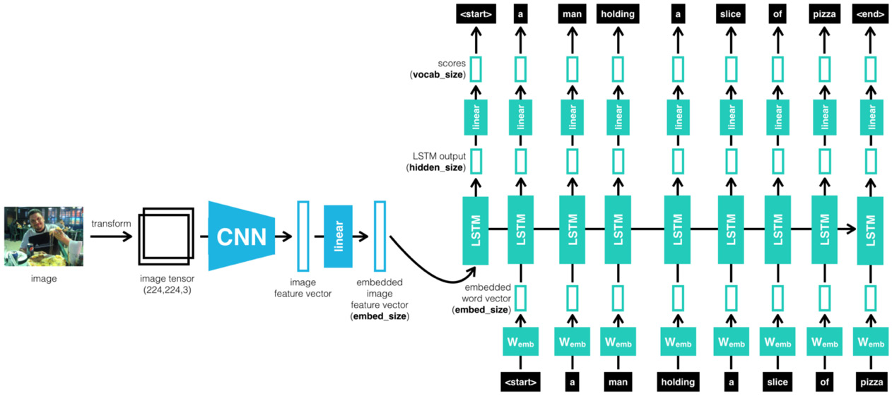
Figure 7.2 – CNN–RNN cascaded architecture

Intuitively speaking, the model is trained to recognize the images and their sentence descriptions so that it learns about the intermodal correspondence between language and visual data. It uses a CNN and a multimodal RNN to generate descriptions of the images. As mentioned above, LSTM is used for the implementation of the RNN.

This architecture was first proposed by Andrej Karpathy and his doctoral advisor Fei-Fei Li in their 2015 Stanford paper titled Generative Text Using Images and Deep Visual-Semantic Alignments for Generating Image Descriptions:

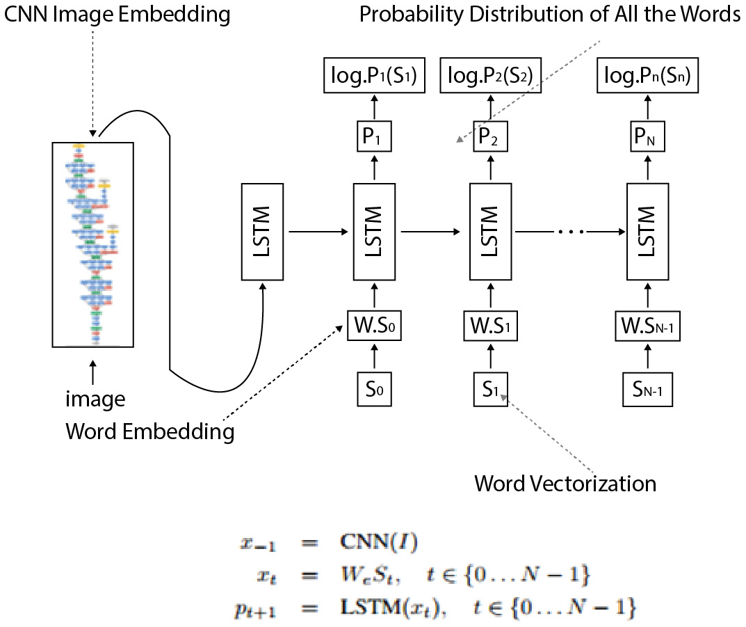
Figure 7.3 – LSTM and CNN working details (Image Credit- Andrej Karpathy)

Let's quickly go through the steps involved in the architecture described in the paper:

1. The dataset contains sentences that are written by people that describe what is happening in the images. The core idea relies on the fact that people will make frequent references to some objects but the context in which they occur. For example, the sentence Man is sitting on the bench has multiple parts, the man being the object, the bench being the location, and sitting being the action. Together, they define the context for the overall image.
2. Our objective is to generate text that describes what is happening in the image as a human would. In order to do so, we need to move the problem to a latent space and create a latent representation of image regions and words. Such a multimodal embedding will create a semantic map of similar contexts together and can generate text for unseen images.
3. In order to achieve it, we first use a CNN as an encoder and get a feature from the last layer before Softmax. In order to extract the relationship between the image and word, we will need to represent the words in the same form of image vector embedding. Thus, the tensor representation of an image is then passed on to an RNN modal.
4. The architecture uses an LSTM architecture to implement the RNN. The specific bidirectional RNN takes a sequence of words and transforms each word into a vector. The LSTM for text generation works a lot like what we saw for time series in Chapter 5, Time Series Models, by predicting the next word in a sentence. It does so by predicting each letter at a time given the entire history of previous letters, picking the letter with the maximum probability.
5. The LSTM activation function is set to a Rectified Linear Unit (ReLU), The training of the RNN is exactly the same as described in the previous model. Finally, an optimization method is used, which is the Stochastic Gradient Descent (SGD), with mini-batches to optimize the model.
6. Finally, in order to generate descriptive text or caption for unseen images, the model works by first using a CNN image recognition model to detect object areas and identify the objects. These objects then become a primer or a seed to our LSTM model and the model predicts the sentence. The sentence prediction happens one character at a time by picking up the maximum probability (Softmax) of a character over the distribution. The vocabulary supplied plays a key part in what text can be generated.
7. And if you change the vocabulary from, say, a caption to poems, then the model will learn to generate the poems. If you give it Shakespeare, it will generate sonnets, and whatever you can imagine!

Generating captions for images

This model will involve the following steps:

1. Downloading the dataset
2. Assembling the data
3. Training the model
4. Generating the caption

Downloading the dataset

In this step, we will download the COCO dataset that we will use to train our model.

COCO dataset

The COCO dataset is a large-scale object detection, segmentation, and captioning dataset (https://cocodataset.org). It has 1.5 million object instances, 80 object categories, and 5 captions per image. You can explore the dataset at https://cocodataset.org/#explore by filtering on one or more object types, such as the images of dogs shown in the following screenshot. Each image has tiles above it to show/hide URLs, segmentations, and captions:

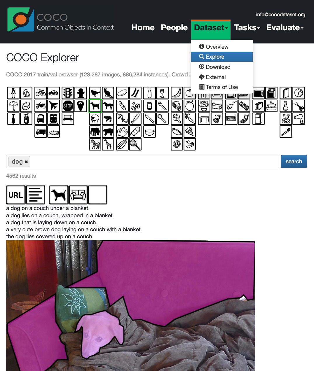
Figure 7.4 – COCO dataset

Here are a few more images from the dataset:

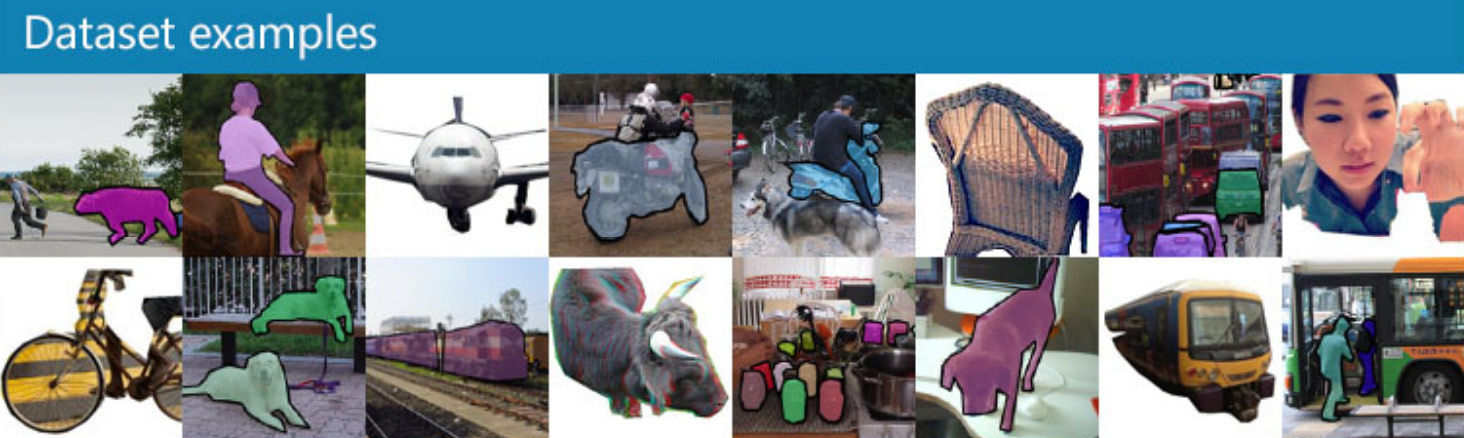
Figure 7.5 – Random dataset examples from the COCO website home page

Extracting the dataset

In this chapter, we will train our hybrid CNN–RNN model using 4,000 images in the COCO 2017 training dataset along with the captions for those images. The COCO 2017 dataset contains more than 118,000 images and more than 590,000 captions. Training a model using such a big dataset takes a very long time, so we filter out 4,000 images and their associated captions, which we will describe later. But first, the following are the steps in code (Downloading_the_dataset.ipynb notebook) for downloading all the images and captions to a folder named coco_data:

!wget http://images.cocodataset.org/zips/train2017.zip

!wget http://images.cocodataset.org/annotations/annotations_trainval2017.zip

!mkdir coco_data

!unzip ./train2017.zip -d ./coco_data/

!rm ./train2017.zip

!unzip ./annotations_trainval2017.zip -d ./coco_data/

!rm ./annotations_trainval2017.zip

!rm ./coco_data/annotations/instances_val2017.json

!rm ./coco_data/annotations/captions_val2017.json

!rm ./coco_data/annotations/person_keypoints_train2017.json

!rm ./coco_data/annotations/person_keypoints_val2017.json

In the preceding code snippet, we download the ZIP files from the COCO website using the wget command. This is equivalent to downloading the files, marked using red arrows in the following screenshot, taken from the download page of the COCO website (https://cocodataset.org/#download):

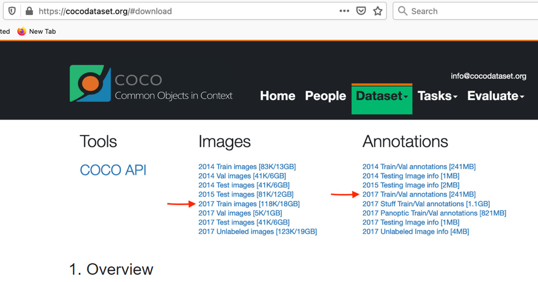
Figure 7.6 – Download page from the COCO website

We unzip the ZIP files and then delete them. We also delete some extracted files that we are not going to use, such as the files containing validation data.

The following screenshot shows the contents of the coco_data directory after running the code snippet:

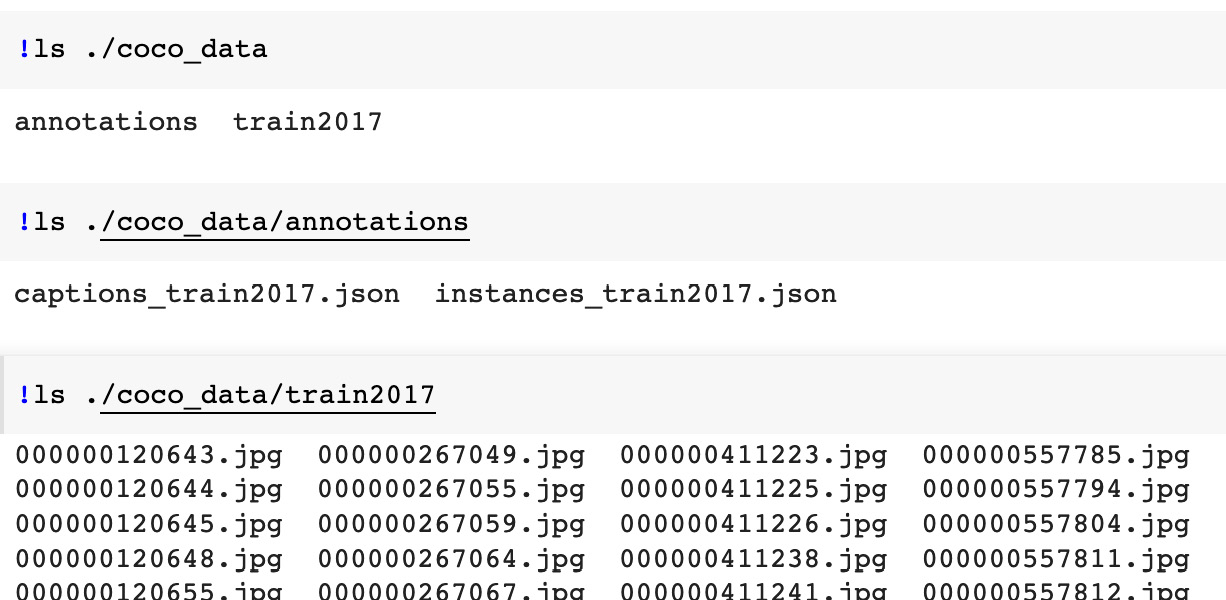
Figure 7.7 – Downloaded and extracted COCO data

Assembling the data

While Deep Learning usually involves large datasets, such as all images and captions in COCO 2017, training a model using such a big dataset requires powerful machines and lots of time. We limit the dataset to 4,000 images and their captions so that the model described in this chapter can be trained in days rather than weeks.

In this section, we will describe how we process the COCO 2017 data in order to filter out 4,000 images and their captions, resize the images, and create the vocabulary from the captions. We will work in the Assembling_the_data.ipynb notebook. We import the necessary packages into the first cell of the notebook, as shown in the following code block:

import os

import json

import random

import nltk

import pickle

from shutil import copyfile

from collections import Counter

from PIL import Image

from vocabulary import Vocabulary

Filtering the images and their captions

As mentioned in the previous section, we limit the size of the training dataset by filtering out 1,000 images each for four categories: motorcycle, airplane, elephant, and tennis racket. We also filter out captions for those images.

First, we process annotations in the instances_train2017.json metadata file. This file has the object detection information (you can refer to details of this and other COCO dataset annotations at the following web page: https://cocodataset.org/#format-data). We use category_id, image_id, and area fields in an object detection annotation for the following two purposes:

• To list various categories that are present in an image.
• To sort categories in an image in decreasing order of their areas. This helps us determine during filtering whether a category is prominent in an image or not. For example, the tennis racket marked in green color in the following figure in the COCO dataset is not as prominent as the people, cars, luggage, and so on. So captions for the image don't mention the tennis racket:

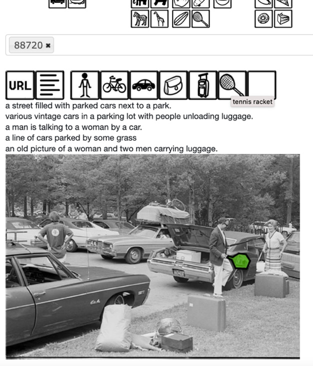
Figure 7.8 – Non-predominant category

Selecting images by categories

In the following code snippet, we start by reading the JSON file and initializing variables:

obj_fl = "./coco_data/annotations/instances_train2017.json"

with open(obj_fl) as json_file:

  object_detections = json.load(json_file)

CATEGORY_LIST = [4, 5, 22, 43]

COUNT_PER_CATEGORY = 1000

category_dict = dict()

for category_id in CATEGORY_LIST:

  category_dict[category_id] = dict()

all_images = dict()

filtered_images = set()

For CATEGORY_LIST, we manually looked up id of the four categories in the categories array in the JSON. For example, the following is an entry for a category (you can select any categories that you wish):

{"supercategory": "vehicle","id": 4,"name": "motorcycle"}

Then, we use the for loop in the following code block to populate the all_images and category_dict dictionaries:

for annotation in object_detections['annotations']:

  category_id = annotation['category_id']

  image_id = annotation['image_id']

  area = annotation['area']

  if category_id in CATEGORY_LIST:

    if image_id not in category_dict[category_id]:

      category_dict[category_id][image_id] = []

  if image_id not in all_images:

    all_images[image_id] = dict()

  if category_id not in all_images[image_id]:

    all_images[image_id][category_id] = area

  else:

    current_area = all_images[image_id][category_id]

    if area > current_area:

      all_images[image_id][category_id] = area

After execution of this for loop, the dictionaries are as follows:

• The all_images dictionary contains categories and their areas for each image in the dataset.
• The category_dict dictionary contains all images that have one or more of the four categories that we are interested in.

If COUNT_PER_CATEGORY is set to -1, it means that you want to filter all images of the categories specified in CATEGORY_LIST. So, in the if block, we just use category_dict to get images.

Otherwise, in the else block, we filter out the COUNT_PER_CATEGORY number of prominent images for each of the four categories. We use two for loops in the else block. The first for loop, shown in the following code block, uses image-specific categories and areas information in the all_images dictionary to sort category_ids for each image in decreasing order of their areas. In other words, after this for loop, a value in the dictionary is a list of categories in decreasing order of their prominence in the image:

for image_id in all_images:

    areas = list(all_images[image_id].values())

    categories = list(all_images[image_id].keys())

    sorted_areas = sorted(areas, reverse=True)

    sorted_categories = []

    for area in sorted_areas:

      sorted_categories.append(categories[areas.index(area)])

    all_images[image_id] = sorted_categories

The second for loop in the else block iterates over images for the four categories stored in category_dict and uses the information stored in the all_images dictionary to filter out the COUNT_PER_CATEGORY number of most prominent images. This for loop prints the following results:

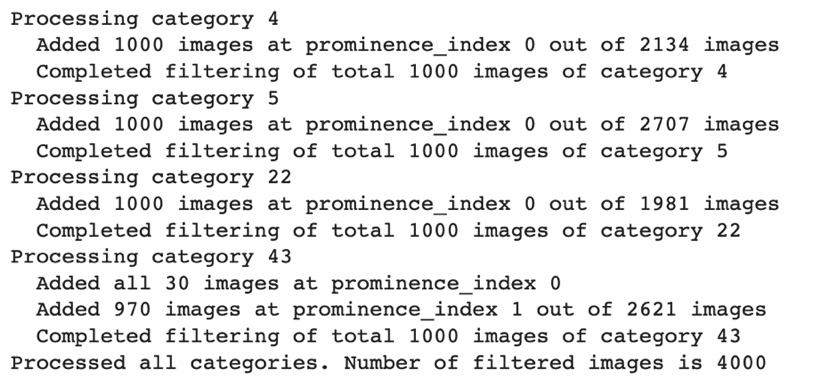
Figure 7.9 – Output from the image filtering code

Selecting captions

In the next cell of the notebook, we start working with the captions stored in the captions_train2017.json metadata file. We separate out captions associated with the images that we filtered in the preceding notebook cell, as shown in the following code block:

filtered_annotations = []

for annotation in captions['annotations']:

  if annotation['image_id'] in filtered_images:

    filtered_annotations.append(annotation)

captions['annotations'] = filtered_annotations

In the JSON file, captions are stored in an array named annotations. A caption entry in the array looks like this:

{"image_id": 173799,"id": 665512,"caption": "Two men herding a pack of elephants across a field."}

We separate out captions whose image_id value is in the filtered_images set.

The captions JSON file also has an array named images. In the next for loop, we shorten the images array to store entries for only the filtered images:

images = []

filtered_image_file_names = set()

for image in captions['images']:

  if image['id'] in filtered_images:

    images.append(image)

    filtered_image_file_names.add(image['file_name'])

captions['images'] = images

Finally, we save the filtered captions in a new file named coco_data/captions.json and we copy filtered image files (using the copyfile function) to a new directory named coco_data/images:

Figure 7.10 – Output from the image filtering code

This completes our data assembly step and gives us a training dataset of 4,000 images and 20,000 captions across 4 categories.

Resizing the images

All images in the COCO dataset are colored, but they can be of various sizes. As described next, all the images are transformed to a uniform size of 3 x 256 x 256 and stored in a folder named images. The following code block is from the resize_images function defined in the Assembling_the_data.ipynb notebook:

def resize_images(input_path, output_path, new_size):

    if not os.path.exists(output_path):

        os.makedirs(output_path)

    image_files = os.listdir(input_path)

    num_images = len(image_files)

    for i, img in enumerate(image_files):

        img_full_path = os.path.join(input_path, img)

        with open(img_full_path, 'r+b') as f:

            with Image.open(f) as image:

                image = image.resize(new_size, Image.ANTIALIAS)

                img_sv_full_path = os.path.join(output_path, img)

                image.save(img_sv_full_path, image.format)

        if (i+1) % 100 == 0 or (i+1) == num_images:

            print("Resized {} out of {} total images.".format(i+1, num_images))

We pass the following arguments to the resize_images function shown in the preceding code block:

• input_path: the coco_data/images folder where we saved 4,000 filtered images from the COCO 2017 training dataset
• output_path: thecoco_data/resized_images folder
• new_size: dimensions [256 x 256]

In the preceding code snippet, we iterate over all images in input_path and resize each image by calling its resize method. We save each resized image to the output_path folder.

Here are the print messages emitted by the resize_images function:

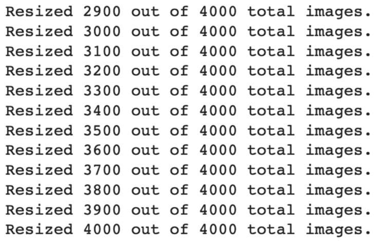
Figure 7.11 – Output for image resizing

Then, in that same notebook cell, we use the following commands to move the resized images into the coco_data/images directory:

!rm -rf ./coco_data/images

!mv ./coco_data/resized_images ./coco_data/images

After the images are resized, we build the vocabulary.

Building the vocabulary

In the last cell of the Assembling_the_data.ipynb notebook, we process the captions associated with the filtered COCO dataset images using the build_vocabulary function. This function creates an instance of the Vocabulary class. The Vocabulary class is defined in a separate file, vocabulary.py, so that the definition can be reused during the training and the prediction phases, as described later. This is why we have added the from vocabulary import Vocabulary statement in the first cell of this notebook.

The following code block shows the Vocabulary class definition in the vocabulary.py file:

class Vocabulary(object):

  def __init__(self):

    self.token_to_int = {}

    self.int_to_token = {}

    self.current_index = 0

  def __call__(self, token):

    if not token in self.token_to_int:

      return self.token_to_int['<unk>']

    return self.token_to_int[token]

  def __len__(self):

    return len(self.token_to_int)

  def add_token(self, token):

    if not token in self.token_to_int:

      self.token_to_int[token] = self.current_index

      self.int_to_token[self.current_index] = token

      self.current_index += 1

We map each unique word – called a token – in the captions to an integer. The Vocabulary object has a dictionary named token_to_int to retrieve the integer corresponding to a token and a dictionary named int_to_token to retrieve the token corresponding to an integer.

The following code snippet shows the definition of the build_vocabulary function in the last cell of the Assembling_the_data.ipynb notebook:

def build_vocabulary(json_path, threshold):

  with open(json_path) as json_file:

    captions = json.load(json_file)

  counter = Counter()

  i = 0

  for annotation in captions['annotations']:

    i = i + 1

    caption = annotation['caption']

    tokens = nltk.tokenize.word_tokenize(caption.lower())

    counter.update(tokens)

    if i % 1000 == 0 or i == len(captions['annotations']):

      print("Tokenized {} out of total {} captions.".format(i, len(captions['annotations'])))

  tokens = [tkn for tkn, i in counter.items() if i >= threshold]

  vocabulary = Vocabulary()

  vocabulary.add_token('<pad>')

  vocabulary.add_token('<start>')

  vocabulary.add_token('<end>')

  vocabulary.add_token('<unk>')

  for i, token in enumerate(tokens):

    vocabulary.add_token(token)

  return vocabulary

vocabulary = build_vocabulary(json_path='coco_data/captions.json', threshold=4)

vocabulary_path = './coco_data/vocabulary.pkl'

with open(vocabulary_path, 'wb') as f:

    pickle.dump(vocabulary, f)

print("Total vocabulary size: {}".format(len(vocabulary)))

We pass the location of the captions JSON (coco_data/captions.json) as the json_path argument to the function and the 4 value as the threshold argument.

First, we use json.load to load the JSON. nltk stands for Natural Language Toolkit. We use NLTK's tokenize.word_tokenize method to split caption sentences into words and punctuation. We use the collections.Counter dictionary object to count the number of occurrences for each token. After processing all captions inside the for loop, we discard the tokens that appear less frequently than the threshold.

We then instantiate the Vocabulary object and add some special tokens to it – <start> and <end> for the start and end of a sentence, <pad> for padding, and <unk>, which is used as the return value when the __call__ method of the Vocabulary object is asked to return an integer for a token that doesn't exist in the token_to_int dictionary. We then add the rest of the tokens to Vocabulary in a for loop.

Important Note

It is important to add the <pad> token to the vocabulary before any other tokens are added because it ensures that 0 is assigned as the integer value for that token. This makes the definition of the <pad> token consistent with the programming logic in coco_collate_fn, where zeros are directly used (torch.zeros()) when creating a batch of padded captions.

Finally, the vocabulary is persisted in the coco_data directory using the pickle.dump method.

Here are the print messages emitted by the build_vocabulary function:

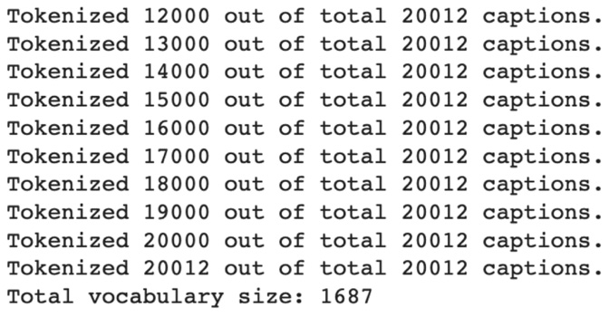
Figure 7.12 – Output of tokenization

After this step, we are ready to start training the model.

Important Note

Downloading the dataset and assembling the data are one-time processing steps. If you are rerunning the model to resume or restart the training, then you do not need to repeat the steps up to this point and can start beyond this point.

Training the model

In this section, we describe the model training. It involves loading data using the torch.utils.data.Dataset and torch.utils.data.DataLoader classes, defining the model using the pytorch_lightning.LightningModule class, setting the training configuration, and launching the training process using the PyTorch Lightning framework's Trainer. We will work in the Training_the_model.ipynb notebook and the model.py file in this section.

We import the necessary packages into the first cell of the Training_the_model.ipynb notebook, as shown in the following code block:

import os

import json

import pickle

import nltk

from PIL import Image

import torch

import torch.utils.data as data

import torchvision.transforms as transforms

import pytorch_lightning as pl

from model import HybridModel

from vocabulary import Vocabulary

Dataset

Next, we define the CocoDataset class, which extends the torch.utils.data.Dataset class. CocoDataset is a map-style dataset, so we define the __getitem__() and __len__() methods in the class. The __len__() method returns a total number of samples in the dataset, whereas the __getitem__() method returns a sample at a given index (the idx parameter of the method, as shown in the following code block):

class CocoDataset(data.Dataset):

    def __init__(self, data_path, json_path, vocabulary, transform=None):

        self.image_dir = data_path

        self.vocabulary = vocabulary

        self.transform = transform

        with open(json_path) as json_file:

            self.coco = json.load(json_file)

        self.image_id_file_name = dict()

        for image in self.coco['images']:

            self.image_id_file_name[image['id']] = image['file_name']

    def __getitem__(self, idx):

        annotation = self.coco['annotations'][idx]

        caption = annotation['caption']

        tkns = nltk.tokenize.word_tokenize(str(caption).lower())

        caption = []

        caption.append(self.vocabulary('<start>'))

        caption.extend([self.vocabulary(tkn) for tkn in tkns])

        caption.append(self.vocabulary('<end>'))

        image_id = annotation['image_id']

        image_file = self.image_id_file_name[image_id]

        image_path = os.path.join(self.image_dir, image_file)

        image = Image.open(image_path).convert('RGB')

        if self.transform is not None:

            image = self.transform(image)

        return image, torch.Tensor(caption)

    def __len__(self):

        return len(self.coco['annotations'])

As described later in this section, __init__ receives the images directory (coco_data/images) as the data_path parameter and the captions JSON (coco_data/captions.json) as the json_path parameter. It also receives the Vocabulary object. The captions JSON is loaded using json.load and stored in the self.coco variable. The for loop in __init__ creates a dictionary named self.image_id_file_name that maps the image ID to a filename.

__len__() returns the total length of the dataset, as shown previously.

Important Note

The COCO dataset has five captions per image. Since our model processes each image-caption pair, the length of the dataset equals the total number of captions, not the total number of images.

The __getitem__() method in the preceding code block returns an image–caption pair for a given index. It retrieves the caption corresponding to the idx index, tokenizes the captions, and uses vocabulary to convert the tokens into their corresponding integers. Then, it retrieves the image ID corresponding to idx, uses the self.image_id_file_name dictionary to get the image's filename, loads the image from the file, and transforms the image based on the transforms parameter.

The CocoDataset object is passed as an argument to DataLoader, as described later in this section. But DataLoader also requires a collate function, which we will describe next.

The collate function

We define the collate function named coco_collate_fn() in the next cell of the Training_the_model.ipynb notebook. As shown in the following code snippet, coco_collate_fn() receives a batch of images and their corresponding captions as input, named data_batch. It adds padding to the captions in the batch:

def coco_collate_fn(data_batch):

  data_batch.sort(key=lambda d: len(d[1]), reverse=True)

  imgs, caps = zip(*data_batch)

  imgs = torch.stack(imgs, 0)

  cap_lens = [len(cap) for cap in caps]

  padded_caps = torch.zeros(len(caps), max(cap_lens)).long()

  for i, cap in enumerate(caps):

    end = cap_lens[i]

    padded_caps[i, :end] = cap[:end]

  return imgs, padded_caps, cap_lens

We first sort data_batch by caption length in descending order, and then we separate the image (imgs) and caption (caps) lists.

Let's denote the length of the imgs list using <batch_size>. It contains 3 x 256 x 256-dimensional images. It is converted into a single tensor of <batch_size> x 3 x 256 x 256 size using the torch.stack() function.

Similarly, the caps list has a total of <batch_size> number of entries and it contains captions of various length. Let's denote the length of the longest caption in a batch using <max_caption_length>. The for loop converts the caps list into a single tensor named padded_caps of <batch_size> x <max_caption_length> size. Captions that are shorter than <max_caption_length> get padded with zeros.

Finally, the function returns imgs, padded_caps, and cap_lens; the cap_lens list contains actual (non-padded) lengths of captions in the batch.

The CocoDataset object and coco_collate_fn() are passed as arguments to DataLoader, as described in the next section.

DataLoader

The get_loader() function is defined in the next cell of the Training_the_model.ipynb notebook, as shown in the following code block:

def get_loader(data_path, json_path, vocabulary, transform, batch_size, shuffle, num_workers=0):

    coco_ds = CocoDataset(data_path=data_path,

                        json_path=json_path,

                        vocabulary=vocabulary,

                        transform=transform)

    coco_dl = data.DataLoader(dataset=coco_ds,

                            batch_size=batch_size,

                            shuffle=shuffle,

                            num_workers=num_workers,

                            collate_fn=coco_collate_fn)

    return coco_dl

The function instantiates a CocoDataset object named coco_ds and passes it, as well as the coco_collate_fn function, as arguments during the instantiation of an object named coco_dl of torch.utils.data.DataLoader type. Finally, the function returns the coco_dl object.

Hybrid CNN–RNN model

The model is defined in a separate file named model.py so that we can reuse the code during the prediction step, as described later. As can be seen in the model.py file, first we import the necessary packages:

import torch

import torch.nn as nn

from torch.nn.utils.rnn import pack_padded_sequence as pk_pdd_seq

import torchvision.models as models

import pytorch_lightning as pl

As always, our HybridModel class extends LightningModule. In the rest of this section, we will describe the CNN and RNN layers, as well as training configurations such as optimizer settings, learning rate, training loss, and batch size.

CNN and RNN layers

Our model is a hybrid of a CNN model and an RNN model. We define sequential layers of both models in __init__() of our HybridModel class definition, as shown in the following code block:

def __init__(self, cnn_embdng_sz, lstm_embdng_sz, lstm_hidden_lyr_sz, lstm_vocab_sz, lstm_num_lyrs, max_seq_len=20):

  super(HybridModel, self).__init__()

  resnet = models.resnet152(pretrained=False)

  module_list = list(resnet.children())[:-1]

  self.cnn_resnet = nn.Sequential(*module_list)

  self.cnn_linear = nn.Linear(resnet.fc.in_features,

                              cnn_embdng_sz)

  self.cnn_batch_norm = nn.BatchNorm1d(cnn_embdng_sz,

                                       momentum=0.01)

  self.lstm_embdng_lyr = nn.Embedding(lstm_vocab_sz,

                                      lstm_embdng_sz)

  self.lstm_lyr = nn.LSTM(lstm_embdng_sz,

                          lstm_hidden_lyr_sz,

                          lstm_num_lyrs,

                          batch_first=True)

  self.lstm_linear = nn.Linear(lstm_hidden_lyr_sz,

                              lstm_vocab_sz)

  self.max_seq_len = max_seq_len

  self.save_hyperparameters()

For the CNN portion, we use the ResNet-152 architecture. We will use a readily available torchvision.models.resnet152 model. However, for output from the CNN model, we don't want a probability prediction that an image is of a given class type such as an elephant or an airplane. Rather, we will use the learned representation of an image output by the CNN, and then it will be passed on as input to the RNN model.

Thus, we remove the last Fully Connected (FC) Softmax layer of the model using the list(resnet.children())[:-1] statement, and then we reconnect all other layers using nn.Sequential(). Then, we add a linear layer named self.cnn_linear, followed by a batch normalization layer named self.cnn_batch_norm. Batch normalization is used as a regularization technique to avoid overfitting and to make the model layers more stable.

Important Note

Note that we pass pretrained=False when instantiating the predefined torchvision.models.resnet152 model in the preceding code snippet. This is because the pretrained ResNet-152 has been trained using the ImageNet dataset, not the COCO dataset, as documented under the ResNet section here: https://pytorch.org/vision/stable/models.html#id10.

You can definitely try using the pretrained=True option as well and explore the accuracy of the model. While a model trained on ImageNet may extract some classes, as shared in Chapter 3, Transfer Learning Using Pre-Trained Models, the overall accuracy may suffer as the complexity of images is quite different in the two datasets. In this section, we have decided to train the model from scratch by using pretrained=False.

For the RNN portion of __init__(), we define LSTM layers, as shown in the preceding code block. The LSTM layers take an encoded image representation from the CNN and output a sequence of words – a sentence containing at most self.max_seq_len words. We use the default value of 20 for the max_seq_len parameter.

Next, we describe the training configuration defined in the HybridModel class in the model.py file.

Optimizer setting

The torch.optim.Adam optimizer is returned by the configure_optimizers method of the HybridModel class, as shown in the following code snippet:

def configure_optimizers(self):

    params = list(self.lstm_embdng_lyr.parameters()) +

             list(self.lstm_lyr.parameters()) +

             list(self.lstm_linear.parameters()) +

             list(self.cnn_linear.parameters()) +

                 list(self.cnn_batch_norm.parameters())

    optimizer = torch.optim.Adam(parameters, lr=0.0003)

    return optimizer

We pass lr=0.0003 as an argument when instantiating the torch.optim.Adam optimizer. lr stands for learning rate.

Important Note

There are dozens of optimizers you can use. The choice of an optimizer is a very important hyperparameter and has a big impact on how a model is trained. Getting stuck in local minima is often a problem, and a change of optimizer is the first thing to try in such cases. You can find a list of all supported optimizers here: https://pytorch.org/docs/stable/optim.html

Changing to an RMSprop optimizer

You can also change the Adam optimizer in the preceding statement to RMSprop, as shown in the following:

optimizer = torch.optim.RMSprop(parameters, lr=0.0003)

RMSprop has a special relationship with sequence generation models such as this one. The centered version first appears in a paper by Geoffrey Hinton titled Generating Sequences With Recurrent Neural Networks (https://arxiv.org/pdf/1308.0850v5.pdf) and has given really good results for caption generation-type problems. It works great in avoiding the local minima for this kind of model. The implementation takes the square root of the gradient average before adding epsilon.

Why one optimizer works better in some cases than others is still a bit of mystery in Deep Learning. In this chapter, for your learning, we have implemented the training using both Adam and RMSprop optimizers. This should prepare you for future endeavors and when trying out various other optimizers.

Training loss

Now, we will define the training loss, for which we will use the cross-entropy loss function.

The training_step() method of the HybridModel class uses torch.nn.CrossEntropyLoss to calculate the loss, as shown in the following code block:

def training_step(self, batch, batch_idx):

    loss_criterion = nn.CrossEntropyLoss()

    imgs, caps, lens = batch

    outputs = self(imgs, caps, lens)

    targets = pk_pdd_seq(caps, lens, batch_first=True)[0]

    loss = loss_criterion(outputs, targets)

    self.log('train_loss', loss, on_epoch=True)

    return loss

The batch parameter of the training_step() method is nothing but the values returned by coco_collate_fn described earlier, so we assign those values as such. They are then passed to the forward method to generate the outputs, as can be seen in the outputs = self(imgs, caps, lens) statement. The targets variable is used to calculate the loss.

The self.log statement uses the logging feature of the PyTorch Lightning framework to record the loss. That is how we are able to retrieve the loss curve, shown later when we describe the training process.

Important Note

Refer to the Managing training section of Chapter 10, Scaling and Managing Training for details of how the loss curve is visualized in TensorBoard.

Learning rate

As we mentioned earlier, you can change the lr learning rate in the following statement in the configure_optimizers() method of the HybridModel class:

optimizer = torch.optim.Adam(params, lr=0.0003)

Important Note

As documented at https://pytorch.org/docs/stable/generated/torch.optim.Adam.html#torch.optim.Adam, the default lr value is 1e-3, that is, 0.001. We have changed the lr value to 0.0003 to converge better.

Batch size

On the other hand, using a bigger batch size enables you to use a higher learning rate that reduces the training time. You can change the batch size at the following statement in Training_the_model.ipynb where the get_loader() function is used to instantiate DataLoader:

coco_data_loader = get_loader('coco_data/images',

                              'coco_data/captions.json',

                              vocabulary,

                              transform,

                              256,

                              shuffle=True,

                              num_workers=4)

The batch size in the preceding code snippet is 256.

The sentence output by the LSTM should ideally describe the image input to the CNN after HybridModel is trained. In the next step, we describe how the Trainer provided by the PyTorch Lightning framework is used to launch model training. We also describe how coco_data_loader, described in the preceding code snippet, is passed as an argument to Trainer.

Launching model training

We worked on the model.py file in the previous section regarding the HybridModel class. Now, back in the Training_the_model.ipynb notebook, we will work in the last cell of the notebook, as shown in the following code block:

transform = transforms.Compose([

    transforms.RandomCrop(224),

    transforms.RandomHorizontalFlip(),

    transforms.ToTensor(),

    transforms.Normalize((0.485, 0.456, 0.406),

                          (0.229, 0.224, 0.225))])

with open('coco_data/vocabulary.pkl', 'rb') as f:

    vocabulary = pickle.load(f)

coco_data_loader = get_loader('coco_data/images',

                              'coco_data/captions.json',

                              vocabulary,

                              transform,

                              128,

                              shuffle=True,

                              num_workers=4)

hybrid_model = HybridModel(256, 256, 512,

                           len(vocabulary), 1)

trainer = pl.Trainer(max_epochs=5)

trainer.fit(hybrid_model, coco_data_loader)

During training, image preprocessing and normalization transforms specified in the transform variable are performed as required for the pretrained ResNet CNN model. The transform variable is passed as an argument to the get_loader() function that we described in a previous section.

Then, Vocabulary, persisted using pickle, is loaded from the coco_data/vocabulary.pkl file.

Next, a DataLoader object named coco_data_loader is created by calling the get_loader function described earlier.

Then, an instance of HybridModel named hybrid_model is created, and the model training is kicked off using trainer.fit(). As shown in the preceding code block, we pass hybrid_model as well as coco_data_loader as arguments to the fit method. The following is a screenshot of output produced by PyTorch Lightning during the training:

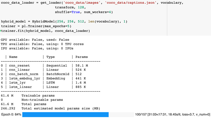
Figure 7.13 – Training output

Important Note

As you may have noticed, we only train the model for five epochs by setting max_epochs=5 during instantiation of pl.Trainer, as shown in the preceding code snippet. For realistic results, the model would need to be trained for thousands of epochs on a GPU machine in order to converge, as shown in the next section.

Training progress

In order to boost the speed of model training, we used GPUs and turned on the 16-bit precision setting of the PyTorch Lightning Trainer, as shown in the following code statement. If your underlying infrastructure has GPUs, then that option can be enabled using the gpu=n option where n is the number of GPUs to be used. To use all available GPUs, specify gpu=-1, as shown here:

trainer = pl.Trainer(max_epochs=50000,

                     precision=16, gpus=-1)

Using a lower learning rate helps the model train better, but training takes more time. The following chart shows the loss curve for lr=0.0003 using black- colored arrows, compared to the other curve for lr=0.001:

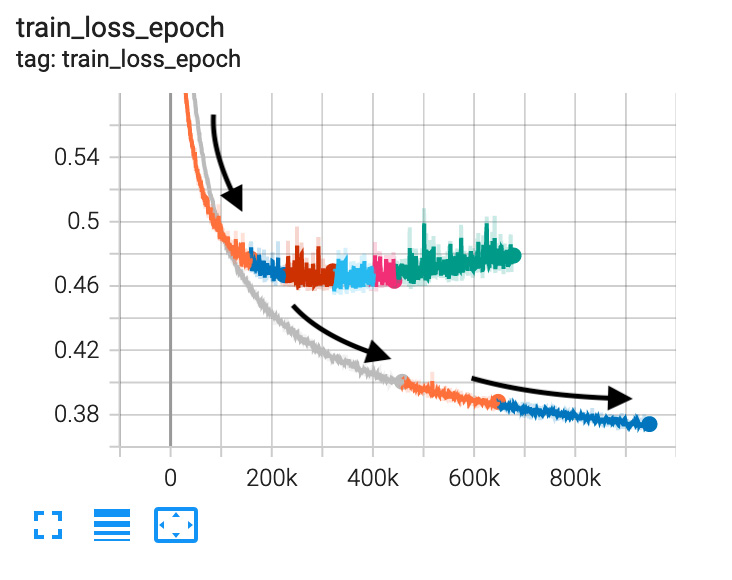
Figure 7.14 – Loss trajectory with different learning rates – the lower the better

Training with the RMSprop optimizer shows us a good decline in the loss rate, as shown in the following chart:

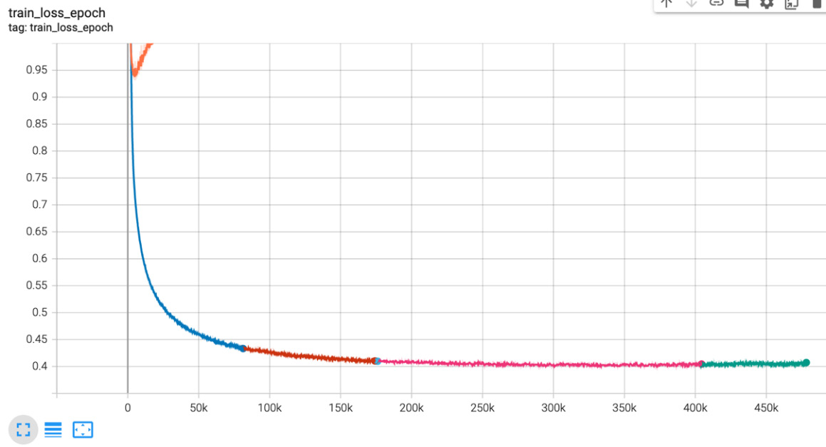
Figure 7.15 – Training loss with RMSprop

Generating the caption

Our HybridModel definition in the model.py file has a couple of peculiar implementation details necessary for it to be used for prediction. We will describe those peculiarities first, and then we will describe the code in the Generating_the_caption.ipynb notebook.

There is the get_caption method in the HybridModel class, which will be called to generate a caption for an image. This method takes an image as input, makes a forward pass through the CNN to generate the input features for LSTM, and then uses a greedy search to generate the caption with the maximum probability:

def get_caption(self, img, lstm_sts=None):

  """CNN"""

  features = self.forward_cnn_no_batch_norm(img)

  """LSTM: Generate captions using greedy search."""

  token_ints = []

  inputs = features.unsqueeze(1)

  for i in range(self.max_seq_len):

    hddn_vars, lstm_sts = self.lstm_lyr(inputs, lstm_sts)

    model_outputs = self.lstm_linear(hddn_vars.squeeze(1))

    _, predicted_outputs = model_outputs.max(1)

    token_ints.append(predicted_outputs)

    inputs = self.lstm_embdng_lyr(predicted_outputs)

    inputs = inputs.unsqueeze(1)

  token_ints = torch.stack(token_ints, 1)

  return token_ints

Also, we have separated part of the CNN's forward logic in a separate method named forward_cnn_no_batch_norm() in the HybridModel class. As shown in the preceding code snippet, this is the method that get_caption uses for the forward pass through CNN in order to generate the input features for LSTM because the cnn_batch_norm module is to be omitted during the prediction phase of a CNN:

def forward_cnn_no_batch_norm(self, input_images):

    with torch.no_grad():

        features = self.cnn_resnet(input_images)

    features = features.reshape(features.size(0), -1)

    return self.cnn_linear(features)

For the remainder of this section, we will work in the Generating_the_caption.ipynb notebook. First, we import the necessary packages in the first cell of the notebook, as shown in the following code block:

import pickle

import numpy as np

from PIL import Image

import matplotlib.pyplot as plt

import torchvision.transforms as transforms

from model import HybridModel

from vocabulary import Vocabulary

In the second cell of the notebook, we use the load_image function to load the image, transform it, and display it, as shown in the following code snippet:

def load_image(image_file_path, transform=None):

    img = Image.open(image_file_path).convert('RGB')

    img = img.resize([224, 224], Image.LANCZOS)

    plt.imshow(np.asarray(img))

    if transform is not None:

        img = transform(img).unsqueeze(0)

    return img

# Prepare an image

image_file_path = 'sample.png'

transform = transforms.Compose([

    transforms.ToTensor(),

    transforms.Normalize((0.485, 0.456, 0.406),

                         (0.229, 0.224, 0.225))])

img = load_image(image_file_path, transform)

Then, we create an instance of HybridModel by passing the checkpoint to HybridModel.load_from_checkpoint(), as shown in the following code block:

hybrid_model = HybridModel.load_from_checkpoint("lightning_logs/version_0/checkpoints/epoch=4-step=784.ckpt")

token_ints = hybrid_model.get_caption(img)

token_ints = token_ints[0].cpu().numpy()

# Convert ints to strings

with open('coco_data/vocabulary.pkl', 'rb') as f:

    vocabulary = pickle.load(f)

predicted_caption = []

for token_int in token_ints:

    token = vocabulary.int_to_token[token_int]

    predicted_caption.append(token)

    if token == '<end>':

        break

predicted_sentence = ' '.join(predicted_caption)

# Print out the generated caption

print(predicted_sentence)

We pass the transformed image to the get_caption method of the model. The get_caption method returns integers corresponding to tokens in the caption, so we use vocabulary to get the tokens and generate the caption sentence. We finally print the caption.

Image caption predictions

Now we can pass an unseen image (which was not part of the training set) and ask the model to generate the caption for us. While the sentence generated by our model is not yet perfect (it might take tens of thousands of epochs to converge), a quick search in the captions.json file for this entire sentence reveals that the model created the sentence on its own. The sentence is not part of the input data that we used to train the model.

Intermediate results

The model works by understanding classes from the image and then generating the text using the RNN LSTM model for those classes and subclass actions. You will notice some noise in earlier predictions.

The following are the results after 200 epochs:

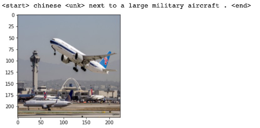
Figure 7.16 – Results after 200 epochs

The following are the results after 1,000 epochs:

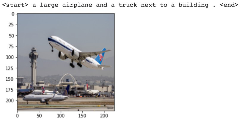
Figure 7.17 – Results after 1,000 epochs

The following are the results after 2,000 epochs:

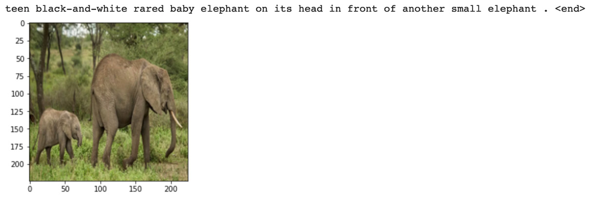
Figure 7.18 – Additional results after 2000 epochs

Results

You may find that after 10,000 epochs, generated captions start getting more human-like. The results will continue to get better with even more epochs. However, don't forget that we have trained this model on only a 4,000-image set. That limits the scope of all the contexts and English vocabulary it can learn from. If this were to train on millions of images, then results on unseen images would be much better.

We trained this model on a GPU server and it took us over 4 days to complete. Here are some caption predictions on RMSprop after 7,000 epochs with a batch size of 256 and learning rate of 0.001:

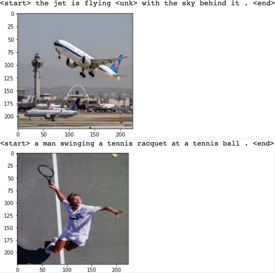
Figure 7.19 – Results after 7000 epochs with RMSprop

The results for the same after 10,000 epochs comes out to be the following:

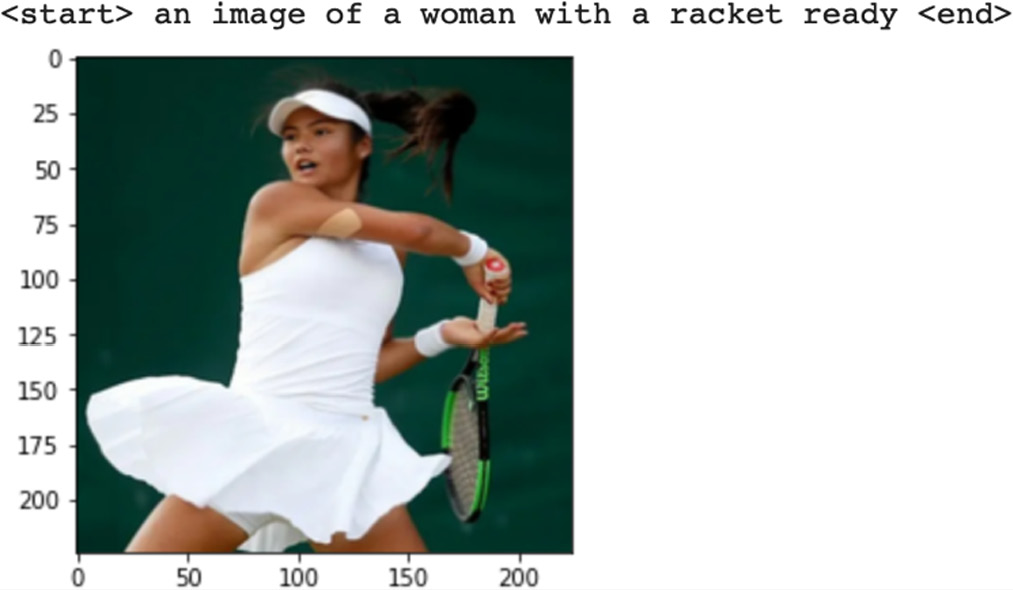
Figure 7.20 – Results after 10,000 epochs

As you can see, we are getting interesting results for our model, especially with higher epochs. Now we can ask the machine to generate captions as a human would.

Next steps

Now that we have shown how a machine can generate captions for images, as an additional exercise, you can try the following to improve your skills:

• Try various other training parameter combinations, such as a different optimizer, learning rate, or a number of epochs.
• Try changing the CNN architecture from ResNet-152 to ResNet-50 or other like AlexNet or VGGNet.
• Try the project with a different dataset. There are other datasets available in the semi-supervised domain with application-specific captions, such as the manufacturing sector or medical images.
• As shown in an earlier section regarding the introduction of semi-supervised learning, instead of generating captions in plain English, you can use any style, such as poems or texts by Shakespeare, by first training the model on those texts and then using a style-transfer mechanism to generate the caption. To recreate the results shown earlier, you could train on a lyrics dataset and ask machine to emulate their poetic style.
• Finally, to expand your horizons even more, you could try combining other models. Audio is also a form of sequence, and you can try models that generate audio commentary automatically for some given images.

Summary

We have seen in this chapter how PyTorch Lightning can be used to create semi-supervised learning models easily with a lot of out-of-the-box capabilities. We have seen an example of how to use machines to generate the captions for images as if they were written by humans. We have also seen an implementation of code for an advanced neural network architecture that combines the CNN and RNN architectures.

Creating art using machine learning algorithms opens new possibilities for what can be done in this field. What we have done in this project is a modest wrapper around recently developed algorithms in this field, extending them to different areas. One challenge in generated text that often comes up is a contextual accuracy parameter, which measures the accuracy of created lyrics based on the question, does it make sense to humans? The proposal of some sort of technical criterion to be used to measure the accuracy of such models in this regard is a very important area of research for the future.

This idea of multi-modal learning can also be extended to video with audio. There is a strong correlation in movies between the action taking place onscreen (such as a fight, romance, violence, or comedy) and the background music played. Eventually, it should be possible to extend multimodal learning into the audiovisual domain, predicting/generating background musical scores for short videos (maybe even recreating a Charlie Chaplin movie with its background score generated by machine learning!).

In the next chapter, we will see the newest and perhaps the most advanced learning method, called Self-Supervised Learning. This method makes it possible to do machine learning even on unlabeled data by self-generating its own labels and thereby opening up a whole new frontier in the domain. PyTorch Lightning is perhaps the first framework to have built-in support for Self-Supervised Learning models to make them easily accessible to the data science community, as we will see in the next chapter.