5

Pseudo-randomized Quantizing

Some of the effects caused by the deliberate injection of randomness into signal digitizing procedures are beneficial and some are harmful, increasing statistical errors. Fortunately, the targeted benefits are often obtained at low levels of randomization. Therefore the randomization level should be controlled to suppress additional errors and excessive randomization must, of course, be avoided in all cases. Yet another useful approach to obtaining the desirable effects is substitution of randomization by making deterministic signal digitization processes simply irregular. Such an approach is less harmful and usually leads to obtaining the same positive effects that are expected from the randomization. Pseudo-randomization of quantizing, considered in this chapter, actually represents such an irregularization. Pseudo-randomized quantizing is evidently a fully deterministic process. A description of it in probabilistic and statistical terms is a convenient way to explain that. It is further shown that skilful application of pseudo-randomization techniques leads to quite good results.

5.1 Pseudo-randomization Approach

It may be a little confusing to understand where the line separating randomized and pseudo-randomized quantization should be drawn. To randomize or pseudorandomize quantizing, an element of randomness either has to be added at the input of the used ADC or it has to be used for randomizing the positions of the reference threshold levels used for quantizing, as shown in Figures 5.1(a) and (b) respectively. Pseudo-random number generators (PRNGs) with digital-to-analog converters (DACs) added are typically used for generation of the analog auxiliary pseudo-random processes needed for that. At first glance all three quantizers shown in Figure 5.1 look equivalent. However, there are significant differences between the first two schemes and the third, shown in Figure 5.1(c). While both of the first two schemes depict a randomized quantizer, the third diagram is a scheme of a pseudo-randomized quantizer.

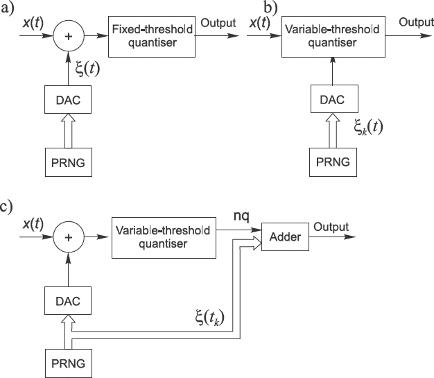
Figure 5.1 Quantizers illustrated by schemes (a) and (b) are randomized and the pseudorandomized quantizer is illustrated by scheme (c)

In all of the illustrated cases the quantizing operation is based on comparing signal instantaneous values with variable thresholds generated by a PRNG together with a DAC. When the quantizing operation is performed in this way, the positions of the threshold levels at all {t_k} are in fact known. Whether this information is used or not is another question, but it is there, given at each t_k even in the digital form. Evidently, this information is not used at randomized quantization when the quantized signal is simply defined as n_kq.

The quantizer shown in Figure 5.1(c) differs distinctly from the other schemes illustrated. There are two components in the output. The quantized signal values provided are defined as a function depending both on n_k and ξ_k (or q_0k). Evidently the auxiliary pseudo-random process in this case is used in quite a different way. It is added to the input signal (this is equivalent to shifting the set of reference threshold levels up or down) and then the same process is used to form the output signal values. As shown below, such a pseudo-randomized quantizer has outstanding properties that cannot be obtained either from deterministic or randomized quantizers. It has the advantages of randomized quantizers without their basic disadvantages.

The question, of course, is exactly how the ξ_k values should be used in the definition of the pseudo-randomized quantization output. To find the answer to this question, an attempt will be made to discover the conditions under which the pseudo-ramdomized quantization operation might be considered to be optimal.

5.2 Optimal Quantizing

Quantizing will be considered optimal if this operation provides the best conditions for estimating the mean value m_x of a signal x(t) ∊ [0, X]. Without loss of generality, an analysis of optimal quantization can be carried out under the assumption that x(t) = x = constant and that only a single threshold level is used for quantization.

5.2.1 Single-threshold Quantizing

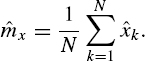
Consider pseudo-randomized quantizing with the information provided by {ξ_k} taken into account. The quantized signal then can be defined as

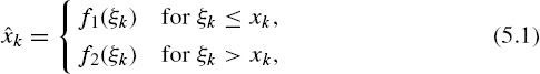
and the estimate of m_x as

Such quantizing should be performed in a way ensuring that the estimate _x is unbiased, i.e. that the following equality holds:

Then

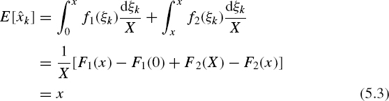
where

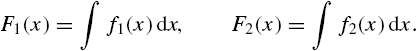
It follows from Equation (5.3) that the functions F₁(x) and F₂(x) should meet the conditions

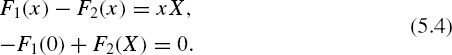
Any functions f₁(ξ) and f₂(ξ) that satisfy Equations (5.4) can be applied in order to define the quantized signal according to Equation (5.1), and all of them will provide unbiased estimates of x. Assume that f₁(ξ) and f₂(ξ) are linear functions

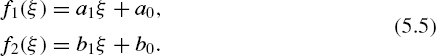
In this case,

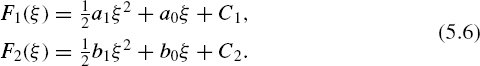
As can be seen from equation (5.3), E[_k] does not depend on the constants C₁ and C₂ and, therefore, they can be considered as equal to zero. Substituting Equation (5.6) into Equation (5.4) gives

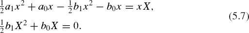
The first of these equations is satisfied for any x if the following conditions are met:

Taking these expressions into account, it follows from Equation (5.7) that

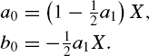
The quantized signal can be defined as follows:

Definition (5.9) holds for a₁ varying within large margins. For instance, when a₁ = 0, this definition describes randomized quantization. Although the estimate _x with a₁ varying remains unbiased, other properties of the quantized signal, including the random error, of course depend on a₁. It is therefore essential to optimize such quantization or, in other words, to find the value of a₁ that provides the minimum of some criterion K.

As the variance Var[] in general depends on x, optimization can be carried out with respect to

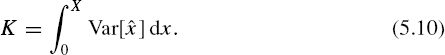
It can be written that

Substituting Equation (5.11) into Equation (5.10) gives

and it is clear that the minimum K_min = X³ is achieved at a₁ = 1. Thus pseudo randomized quantizing provides the minimum of the variance Var[] averaged over x if the quantized signal is defined in the following way:

It can be seen from Equation (5.10) that such quantization is characterized by

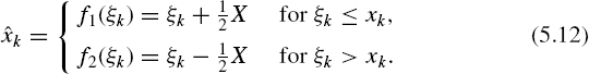
What is important is that this variance does not depend on x. This remarkable property makes the quantization model considered here exceptional. All other quantization models defined by Equation (5.9) are characterized by Var[] depending on x, as shown in Figure 5.2. The curves given there are for the normalized signal values varying within the range of (−1, 1) and five quantization models corresponding to various values of 0 ≤ a₁ ≤ 2.

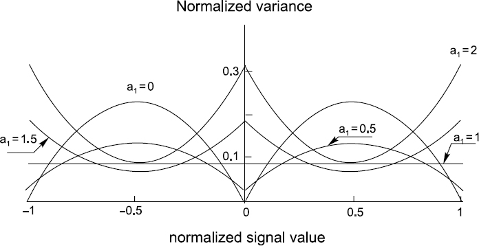
Figure 5.2 Variances of a signal quantized pseudo-randomly in various ways

As optimization of the pseudo-randomized quantization is carried out under the assumption that the functions f₁(ξ_k) and f₂(ξ_k) are linear, it is not clear whether the results are also optimal when these functions are nonlinear. This question has been investigated and it was found that the quantization performed in accordance with equation (5.12) is also optimal when the functions f₁(ξ_k) and f₂(ξ_k) are nonlinear.

5.2.2 Multithreshold Quantizing

Since the quantized signals obtained in the course of pseudo-randomized quantizing are unbiased, no matter how coarse the quantization procedure, all essential relationships characterizing such quantizing are the same both for a single and a multithreshold quantization. In the latter case, it follows from Equation (5.12) that

It is sometimes more convenient to use another version of Equation (5.14):

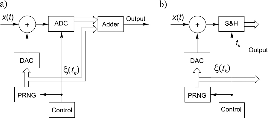
Figure 5.3 Schemes for realizing pseudo-randomized quantizing

As mentioned above, such quantizing is unbiased. Indeed,

Although in this case the reference threshold sets are also formed as described by the quantization Model 2, there is a considerable difference between the quantization performed according to this model and the pseudo-randomized quantization. The quantized signal defined by Equations (5.14) or (5.15) also assumes values, which belong to some discrete levels, but in this case intervals between them are small and equal to the smallest digit of q_0k.

5.2.3 Implementation Approaches

To implement the pseudo-randomized quantization method, it is not necessary to design a completely new type of analog-to-digital converter. Conventional deterministic ADCs can be used to carry out this kind of quantizing, as shown in Figure 5.3. Note that the ADC used should be a high-speed device with a sufficiently small aperture time. To perform pseudo-randomized quantizing according to the scheme given in Figure 5.3(a), the auxiliary random process generated by the pseudo-random number generator (PRNG) is converted by a DAC and the analog random process obtained is added to the input signal. The ADC converts this additive mixture and the digital random variables {ξ_k} are subtracted from the respective values of the ADC's output signal. Thus one and the same random process is added to the input signal and later subtracted from the quantized signal.

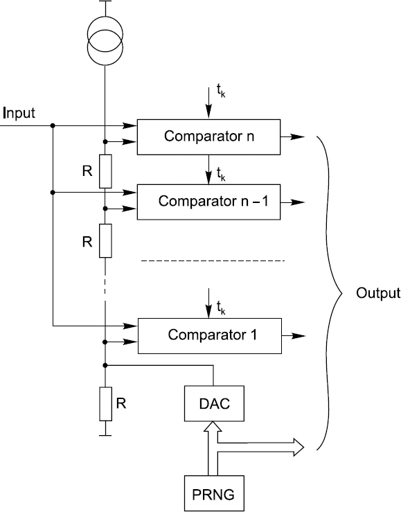
Figure 5.4 A scheme for pseudo-randomized quantising based on application of a flash converter

The operational principle of this scheme is the same as for the optimized quantization mode considered above. When the ADCs used are relatively slow, the scheme in Figure 5.3(a) can be modified as shown in Figure 5.3(b) by adding a sample-and-hold (S&H) circuit.

Another implementation approach is based on the principle of changing the reference threshold levels during the quantization process. A scheme realizing this principle is shown in Figure 5.4. The most vital elements in it are the voltage comparators strobed by short pulses at the sampling time instants {t_k}. The input signal is fed to all inputs of these comparators. The reference inputs are connected to a chain of resistors. Current from a constant current source flowing through this chain of resistors determines the reference voltages or the threshold levels. They depend not only on this current but also on the random voltage across the lowest in the chain resistor R₁, generated by the PRNG in connection with the DAC. The threshold levels at all the comparator reference inputs follow random voltage changes, thus providing the correct operational mode for pseudo-randomized quantizing.

Note that the schemes in Figures 5.3(b) and 5.4 have two rather than one output. This is essential. Output signals of such quantizers can often be processed in two differing ways. They might be passed partly through one processing channel and partly through another. Separate algorithms are used for processing the information carried by the sequence {n_kq} and the information given by the sequence {ξ_k}. It is possible to speed up processing and to simplify the hardware in this way, lessening the negative impact of the main disadvantage of this kind of quantizing: the increased quantity of bits needed for encoding the pseudo-randomly quantized signals.

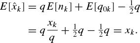
5.3 Input–Output Relationships

Both instantaneous and expected input–output relationships for pseudorandomized quantizing are linear. The point is that the input–expected output relationship is defined in a remarkable way, specifically E [] = x. Instantaneous values of for any value of x all are within a certain area. This means that for all values of x, the respective values are distanced from the corresponding values of E[] by an interval not exceeding ±0.5q. For instance, when x = x₀, the quantized value ₀ can with equal probability assume any value within the interval [x₀ ± 0.5q].

5.4 Quantization Errors

Assume that the quantized signal

Then the conditional probability density function

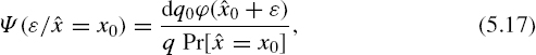
where Pr[ = x₀] is the probability that the quantized signal is equal to x₀. It is obvious that

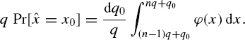
To obtain the unconditional probability density function of ∊, function (5.17) should be averaged over all possible digital values of n = 0, 1, 2,... and over all values of q₀ that are considered to be continuous. Then

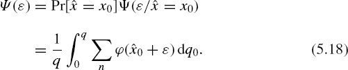
The sum can be expressed by means of δ functions. This can be written as

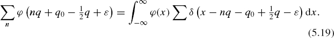
The Fourier transform of the sum of δ functions can be shown to be

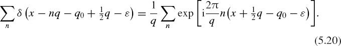
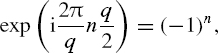
Substituting Equation (5.20) into Equation (5.19) and substituting the result into Equation (5.18) gives

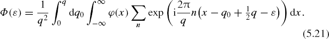
Taking into account the fact that

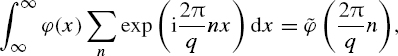
where ((2π/q)n)is the value of the signal characteristic function at the argument equal to (2π/q)n, and that

Equation (5.21) can be rewritten as

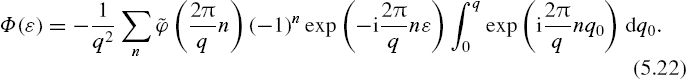
Note that

and (0) = 1. Finally,

This result leads to the following very important conclusion:

Consequently,

Independence of the quantization errors from the input signal simplifies the task of deriving the variance of quantized signals considerably. In this case, it is obvious that

5.5 Quantization Noise

A realization of pseudo-randomized quantization noise is shown in Figure 5.5(d). To obtain an impression of the main properties of this noise, compare it with the deterministic and randomized quantization noises, also given in Figures 5.5(b) and (c).

Comparison of these time diagrams leads to the following conclusions:

1. Pseudo-randomized quantization noise is distributed in an interval [−0.5q, +0.5q]. Therefore, the quantization noise for the pseudo-randomized quantizing does not exceed the boundaries characterizing deterministic quantizing and is distributed in an interval twice smaller than in the case of the noise observed at randomized quantizing of the same signal.
2. An error of pseudo-randomized quantizing at any quantization instant t_k assumes with equal probability any value from the interval [−0.5q, +0.5q].
3. There is no (visible) dependence of the pseudo-randomized quantization noise on the signal being quantized.

The latter conclusion, of course, cannot be based on visual observation. This feature of the pseudo-randomized quantization procedure has to be proved.

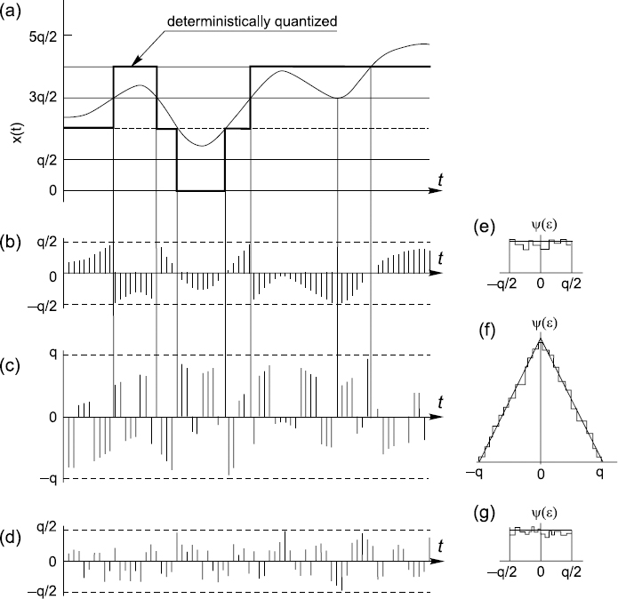
Figure 5.5 Quantizing of a signal in three different ways: (a) input signal with quantization noise and its probability density function; (b), (e) for deterministic quantizing; (c), (f) for randomized; and (d), (g) for pseudo-randomized quantizing

Thus it turns out that pseudo-randomized quantizing is unique. No other known quantization technique has such advantageous properties. At the same time, as might be expected, this quantization approach also has its drawbacks. The most serious disadvantage is the increased number of bits required for representing the quantized signals. At first glance it seems that as a result of this disadvantage the hardware for processing signals quantized in this way should be considerably more complicated than usual. Fortunately, this is not so. As shown in the following chapters, if signal processing is organized on the basis of special algorithms, well matched to the specifics of pseudo-randomized quantizing, the main disadvantage of this kind of quantizing becomes less significant.

5.5.1 Covariance between Signal and Quantization Noise

The quantization noise {∊_k} is divided into two processes, {∊⁽⁺⁾_k and {∊⁽⁻⁾_k} The first process contains only zeroes and positive errors and the second process, similarly, contains zeroes and negative errors. Formally, it can be written that

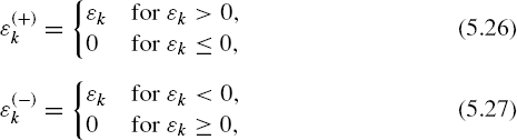
and

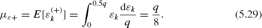
As the pseudo-randomized quantizing errors are distributed uniformly within the interval [−0.5q, +0.5q] independently of the input signal, the expected value of the process {∊⁽⁺⁾_k} is

The covariance between the input signal and the first component of the quantization noise {∊⁽⁺⁾_k} is as follows:

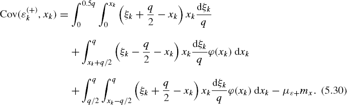
After due integration, and taking into account result (5.29),

Similarly, it can be shown that

Since the input signal is uncorrelated with either noise component, it is obviously also uncorrelated with the quantization noise itself.

5.5.2 Spectrum of the Pseudo-randomized Quantization Noise

In order to determine the spectrum of pseudo-randomized quantization noise, first its autocovariance function C^(p)_∊∊ (mT) will be obtained. As the mean value of this noise m_∊ = 0, then

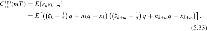
The random variable (ξ_k – ½)q is uniformly distributed within the interval [−0.5q, +0.5q]. Assume that the variables (ξ_k – ½) q and (ξ_k+m – ½)q at m ≠ 0 are mutually independent. Note that (n_kq – x_k) represents errors of randomized quantization.

If these moments are taken into account, it follows from Equation (5.33) that

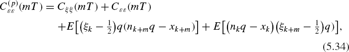
where the autocovariance function of the auxiliary random process C^(p)_∊∊ (mT) = 0 for m ≠ 0, and the autocovariance function of randomized quantization noise C^(p)_∊∊ (mD_t) = 0 for m ≠ 0, as shown in Chapter 4. Then

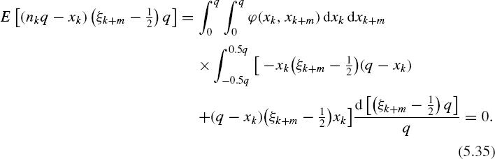
Likewise,

Substituting Equations (5.35) and (5.36) into Equation (5.33) yields

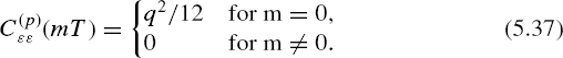
Thus the autocovariance function of the pseudo-randomized quantization noise does not depend on the input signal and is invariable. Consequently, the spectral density function of this noise is

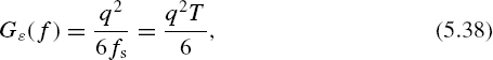
i.e. it is constant over the frequency range [0, 0.5 f_s].

This result leads to the following significant conclusion:

In other words:

No other quantization scheme has a similar property. It is true that randomized quantizing can also be realized in such a way that the quantization noise is white. However, the mean power of this noise depends to some extent on the variance of the input signal. The spectrum of deterministic quantization in principle largely depends on the input signal and this dependence can be weakened only by decreasing the size of the quantization step.

Note that formula (5.38), describing the spectrum of the quantization noise being discussed, is obtained under the assumption that the input signal is sampled periodically. When the signal is sampled randomly, obtaining an analytical description of the respective spectral density function is much more complicated. However, computer simulations show that when expression (5.38) is used for engineering evaluations of the noise spectra, the mean sampling rate f_s can be substituted for the sampling frequency f_s in Equation (5.38).

5.5.3 Noise Reduction by Oversampling

Assume that the spectral density function of a signal x(t) being quantized is confined to the frequency range [0, f₀], f₀ < f_s/2. The power P_∊ of the corresponding rounding-off noise spectrum is distributed evenly over the whole frequency range [0, f_s/2], no matter how rough the quantization is. The spectral density function of this noise can be subdivided into two parts. The first part covers the signal bandwidth and the second part is outside this range. Accordingly, the mean power P_∊ is also divided into two respective parts P₁ and P₂. The mean power of that part of the noise spectrum that belongs to the signal spectrum range is denoted by P₁ and the remaining part by P₂.

Referring to Equation (5.38),

If the quantized signal is passed through a low-pass filter with the cut-off frequency f₀, the second part of the rounding-off noise spectrum power P₂ is filtered out and the resulting quantization accuracy, characterized by the signal-to-noise ratio (SNR) 10 log(P_x/P₁), increases. The SNR can be improved in this way by socalled signal oversampling. If the sampling frequency is increased four times and appropriate filtering applied, the quantization accuracy is improved by one effective bit. This approach is popular and it is used also in the cases of rough deterministic quantization. However then it might be less effective as the power of the deterministic quantization noise at a small number of reference levels used is concentrated more in the low frequency region while it is not so at pseudorandomized quantizing.

5.6 Some Properties of Quantized Signals

The properties of quantized signals naturally differ from the properties of the original signals. These differences depend on the quantization mode applied. This phenomenon has been extensively studied for deterministic quantization applications. This problem has been considered for the case when quantizing is carried out pseudo-randomly.

The moments a_s,r and the central moments μ_s,r of a system of random variables (x,∊) are defined as follows:

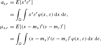
where m_x and m_∊ are the mean values of x and ∊ respectively, ϕ(x, ∊) is the probability density function of the system of the random variables (x, ∊) and Ω is the space of x, ∊ on the plane (x, ∊). As the probability density function of the quantization error ∊ is constant in the interval [−0.5q, 0.5q] and does not depend on ϕ(x), then ϕ(x, ∊) = ϕ(x)Ψ(∊) and

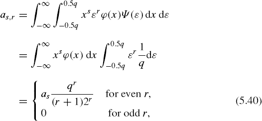
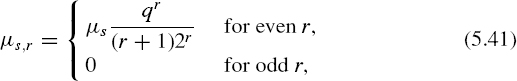
where a_s is the sth moment ϕ(x). Taking into account the fact that m_∊ = 0, then similarly

where μ_s is the 5th central moment of ϕ(x). Now E[^s] can be defined. According to the definition ∊ = x – and

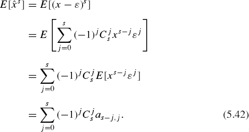
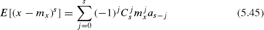
Substituting Equation (5.40) into Equation (5.42) and taking into account the fact that at odd j the moment a_s−j,j is equal to zero and that the sum in Equation (5.42) should be determined only for even j, gives

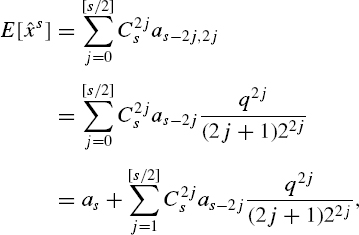
where [s/2] is the integer part of s/2. Hence

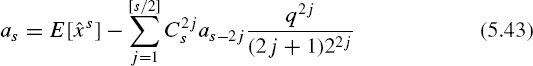
On the basis of Equation (5.43), the following corrections, essential for many engineering calculations, are obtained:

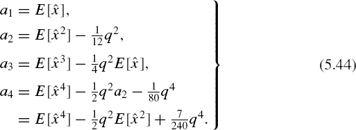
These corrections are the same as those obtained for deterministic quantization, but their meaning is quite different. In the case of deterministically quantized signals, they reduce the bias of the estimates â_s, but their application does not guarantee its elimination. How efficient they are depends on ϕ(x) and on the value of q. When Equations (5.44) are applied for correction of the estimates â_s obtained by processing pseudo-randomly quantized signals, these corrections eliminate bias errors completely, no matter what is the probability density function of the signal or the size of the quantization step q.

To obtain equations describing the estimates â_s of the corresponding moments a_s, the estimates (1/N)Σ^N_k=1 should be substituted for E[_s]. It can be shown that the estimates â_s defined in this way are unbiased. To obtain equations defining the estimates of the central moments μ_s note that on grounds of Equation (5.42),

Table 5.1

and the equation obtained should then be substituted into Equation (5.44). The variance of the estimates ^s is given by

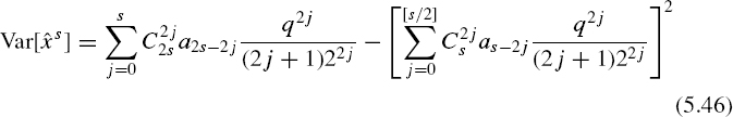
To evaluate the errors of estimating a_s and μ_s, the variance Var[(1/N)Σ^N_{k=1 s}] should be determined first by applying Equation (5.46).

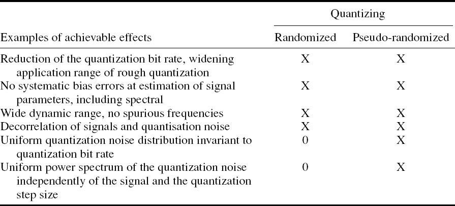
5.7 Benefits

The randomization and pseudo-randomization techniques, considered in Chapters 4 and 5, represent an effective tool for making quantizing flexibly adaptable to specific requirements of an application. Skilful application of randomized and pseudo-randomized quantizing might lead to significant benefits. The most characteristic ones are indicated in Table 5.1.

Although deliberate randomizing and/or pseudo-randomizing of quantizing apparently complicate to some extent the execution of this operation, the approach is also fruitful. The point is that it makes quantizing much better adjusted to the needs and conditions of specific applications and that in turn helps to improve the organization of digital signal processing tasks at hand.

Bibliography

Bennet, W.R. (1948) Spectra of quantized signals. Bell Syst. Tech. J., 27(7), 446–72.

Bilinskis, I. (1976) Stochastic signal quantization error spectrum (in Russian). Autom. Control Comput. Sci., 3, 55–60.

Bilinskis, I. (1977) Quasi-stochastic coding of continuous signals. Pr. Przem. Inst. Elektron., 64, 53–9.

Bilinskis, I. and Mikelsons, A. (1975) Quantizing of signals by parallel stochastic weighting (in Russian). Autom. Control Comput. Sci., 4, 34–8.

Bilinskis, I. and Mikelsons, A. (1992) Randomized Signal Processing. Prentice Hall International (UK) Ltd.

Bilinskis, I., Mikelsons, A. and Nemirovski, R.F. (1974) Application of random point processes for quantizing of time intervals (in Russian). Autom. Control Comput. Sci., 6, 79–85.

Brodsky, P.I., Verjushsky, V.V., Klyushnikov, S.N. and Lutchenko, A.E. (1970) Statistical quantization technique using auxiliary random signals (in Russian). Voprosy Radioelektroniki Ser. obshchetekhnic, 3, 46–53.

Demas, G.D., Barkana, A. and Cook, G. (1973) Experimental verification on the improvement of resolution when applying perturbation theory to a quantizer. IEEE Trans Industr. Electron. Control Instr., IECI20(4), 236–9.

Jayant, N. and Rabiner, L. (1972) The application of dither to the quantization of speech signals. Bell Syst. Tech. J., 51(6), 1293–304.

Roberts, L.G. (1962) Picture coding using pseudo-random noise. IRE Trans. Inf. Theory, IT-8, 145–54.

Veselova, G.P. (1975) On amplitude quantization with overlapping of interpolating signals (in Russian). Avtomatika i Telemekhanika, 5, 52–9.