
CHAPTER 3
Refining Mattes
Regardless of the method used to pull a matte, there are a variety of operations that can be applied to refine the quality of any matte. In this chapter several operations are explored that, among other things, reduce grain noise, soften the edges, and expand or contract the matte size to get a better composite.
3.1 The Matte Monitor
Before we begin, this is a good time to introduce the matte monitor, which you can make with your own color curve tool. Many of the various matte extraction processes result in a raw matte that has to be scaled up to full density. When scaling raw mattes up to full density there can be stray pixels in both the white and black regions of the matte that are hard to see, but will suddenly become very visible in the composite. This can also happen with the mattes from keyers, like Ultimatte. You need a way to see that both your whites and blacks are solid, with no contamination. Here is a little tool you can make with your color curve tool that will make those pesky pixels pop out for you to see—and pound down.
Figure 3-1 shows a supposedly “clean” matte that has hidden bad pixels in both the white and black areas. Figure 3-2 shows how to set up the color curve tool to make a matte monitor. Connect a color curve node to the fully scaled matte or the matte output of a keyer in order to monitor the results. Next, add the two new points shown in Figure 3-2, moving them very close to the left and right margins as shown. Voilà! The bad white and black pixels suddenly become visible like those in Figure 3-3. The zero black and 100 percent white pixels must stay undisturbed, so make certain that both of the end points stay at exactly zero and one.
What this color curve does is find any pixels in the whites that are very nearly white but are hard to see, and pushes them down sharply away from the pure white pixels to make them light gray. Similarly, in the blacks the color curve will push any non-zero pixels up sharply from the true zero black pixels and make them visible. You can leave this node hanging right after a matte scaling operation to make sure you have cleared out all suspect pixels. Of course, the output image is for diagnostic viewing only and is not used in the actual composite. If you are working with proxies, this is an operation that needs to be done at full resolution. Proxies are the low-resolution copies of the full-resolution frames that film compositors create to speed up shot development by avoiding working with the larger (and much slower) full-size frames.
3.2 Garbage Matting
One of the first preprocessing operations to be done on virtually any bluescreen matte extraction process is garbage matting the backing color. The basic idea is to replace the backing area all the way out to the edges of the frame with a clean, uniform color so that when the matte is extracted the backing region will be clean and solid all the way out to the edges of the frame. There are two important criteria to this operation. First, it must replace the bluescreen a safe distance away from the edges of the foreground object. You must make sure that it is the matte extraction process that takes care of the foreground object edges, not the garbage matte. The second criterion is that it not take too much time.
Color Plate 35 shows the original bluescreen plate with an uneven backing color getting darker toward the top of the frame. Color Plate 36 is the garbage matte to be used, and Color Plate 37 is the resulting garbage matted bluescreen. The backing region is now filled with a nice uniform blue, prepped for matte extraction. Notice also that the garbage matte did not come too close to the edges of the foreground.
There are basically two ways to generate the garbage matte (or “g-matte”): procedurally (using rules), and by hand (rotoscope). Obviously, the procedural approach is preferred because it will take very little time. As an opening gambit, try using a chroma-key node to pull a simple chroma-key matte on the backing color. If chromakey is not a viable solution for some reason, you can always use the second method of drawing the garbage mattes by hand, which obviously will be more time consuming. Because we are trying not to get too close to the edges of the foreground object, the rotos can be loosely drawn and perhaps spaced out every 10 frames or so. The two methods can also be combined by using a chroma-key matte for most of the backing region plus a single garbage matte for the far outer edges of the screen, which are often badly lit or have no bluescreen at all.
However you wind up creating it, once the g-matte is ready, simply composite the foreground object over a solid plate of blue. But what blue to use? The RGB values of the backing vary everywhere across its surface. As you can see in the garbage matted bluescreen of Color Plate 37, the color of the filled area is darker than the remaining bluescreen in some areas and lighter in others. You should sample the actual bluescreen RGB values near the most visually important parts of the greenscreen, typically around the head if there is a person in the plate. This way the best matte edges will end up in the most visually important part of the picture.
3.3 Filtering the Matte
In this section we will explore the filtering (a fancy word for blurring) of the matte. There are two main reasons to apply a gentle blur operation to a matte. First, it smooths down the inevitable grain noise. This allows us to reduce somewhat how hard the matte has to be scaled up later to eliminate any “holes” in the finished matte. Second, it softens the edges of the matte. The tendency for all mattes extracted from images is to have too hard an edge. This we can fix, but first let us look into how a gentle blur helps our cause.
3.3.1 Noise Suppression
Even if a bluescreen is degrained before matte extraction there will still be some residual grain noise. If the grain noise needs further suppression, the raw matte can be blurred before it is scaled to full density. The blur operation helps reduce the amount of scaling required to get a clean matte in the first place, and minimal scaling is always desirable.
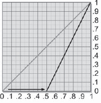
Figure 3-4 is a slice graph of a noisy (grainy) raw matte. The noise causes the pixel values to chatter both up and down. This tends to close the useable gap between the leading region (around 0.3) and the foreground region (near 0), to only about 0.2. This 0.2 region is all that is available for the final scaled matte if you are trying to eliminate the noise by scaling alone.
Figure 3-5 shows the effects of a blur operation. It has smoothed out the noise in both the backing and foreground regions. As a result, the gap has opened up to 0.3, increasing the available raw matte density range by 50 percent. (All numbers have been exaggerated for demo purposes—your results may vary.) If you pull a matte on a nicely shot greenscreen with a minimum amount of noise, you may not have to perform this operation on the raw matte, so feel free to skip it when possible. Remember, the blur operation destroys fine detail in the matte edges, so use it sparingly. A median filter can also be used, which has the advantage of not softening the edges of the matte.
Figure 3-6 shows a flowgraph of a generic matte extraction operation with the blur operation for grain suppression inserted before the matte scaling operation.
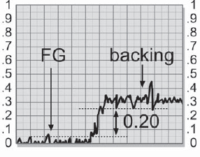
Figure 3-4: Slice Graph of Noisy Raw Matte
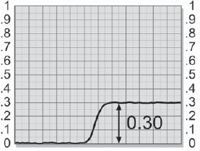
Figure 3-5: Raw Matte after Blur Operation

Figure 3-6: Blur Operation on Raw Matte to Suppress Grain Noise
3.3.2 Softer Edges
When softer edges are needed, the blur operation is performed on the final matte after it has been scaled to full density. The blur softens the composited edge transition in two ways. First, it mellows out any sharp transitions, and second, it widens the edge, which is normally good. It is important to understand what is going on, however, so that when it does introduce problems you will know what to do about them.
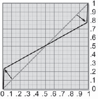
Figure 3-7 shows a slice graph of a matte's edge transition between the white and black regions. The dotted line represents the matte before a blur operation, with the short arrow at the top of the graph marking the width of the edge transition. The steep slope of the dotted line indicates that it is a hard edge. The solid black line represents the matte after a blur operation, and the longer arrow at the bottom marks the new width of the edge transition. The slope of the solid line is shallower, indicating a softer edge. In addition to the softer edge it is also a wider edge.
The blur operation has taken some of the gray pixels of the transition region and mixed them with the black pixels from the backing region, pulling them up from black. Similarly, the white pixels of the foreground region have been mixed with the gray transition pixels, pulling them down. As a result, the edge has spread both inward and outward equally, shrinking the core of the matte while expanding its edges.
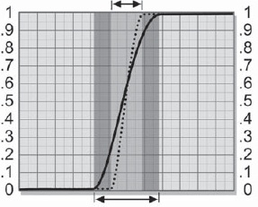
Figure 3-7: Slice Graph of Blurred Final Matte
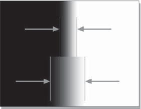
Figure 3-8: Edge Width Before and After Blur Operation
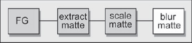
Figure 3-9: Blur Operation on Final Matte to Soften Edges
This edge spreading effect can be seen very clearly in Figure 3-8. The top half is the original edge, and the bottom half is the blurred edge. The borders of the edge have been marked in each version, and the much wider edge after the blur is very apparent. This edge expansion often helps the final composite, but occasionally it hurts it. You need to be able to increase or decrease the amount of blur and shift the edge in and out as necessary for the final composite—and all of this with great precision and control. Not surprisingly, the next section is about such precision and control.
Figure 3-9 shows a flowgraph with the blur operation added after the matte scaling operation for softening the edges of the final matte.
3.3.3 Controlling the Blur Operation
In order to apply the gentlest possible blur operation that will fix the grain problem it is important to understand how blur operations work. There are typically two parameters (controls) used to adjust the effects of a blur operation: the blur radius and the blur percentage. And now, we digress to the nomenclature game. Although most software packages will refer to the blur radius as the “radius” (a few may call it “kernel size”), the parameter I am calling the blur “percentage” can go by many names. Your particular package may call it the “blur factor” or “blur amount,” or something else even less helpful like “more blur.” Let's take a look at each of these two parameters, radius and percentage, and see how they affect the blur operation and how to set them for best results. The main problem we are addressing here is how to knock down the grain without knocking out other important matte details we want to keep. This requires a delicate touch.
3.3.3.1 The Blur Radius
A blur operation works by replacing each pixel in the image with an average of the pixels in its immediate vicinity. The first question is, what is the immediate vicinity? This is what the blur radius parameter is about. The larger the radius, the larger the “immediate vicinity.” To take a clear example, a blur of a radius of 3 will reach out 3 pixels all around the current pixel, average all those pixel values together, then put the results into the current pixel's location. A blur radius of 10 will reach out 10 pixels in all directions, and so on. Not all blur operations use a simple average. There are a number of blur algorithms, each giving a slightly different blur effect. It would be worthwhile to run a few tests with your blur options to see how they behave.
Those packages that refer to “kernel size” will be talking about a square region of pixels with the current pixel at the center, like those in Figure 3-10. For example, a 7 × 7 kernel will have the current pixel in the center of a 7 × 7 grid, and will “reach out” 3 pixels all around it. In other words, it is equivalent to a radius of 3. Note that since the kernel always has the current pixel in the center and gets larger by adding another pixel all around the perimeter, it will only come in odd sizes (3 × 3, 5 × 5, 7 × 7, etc.). While it is technically possible to create kernels of non-odd-integer dimensions (i.e., a 4.2 × 4.2 kernel), some packages don't support it.
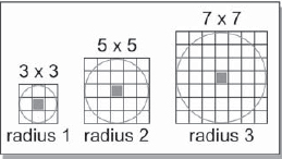
Figure 3-10: Blur Radius versus Blur Kernel
So what is the effect of changing the radius (or kernel size) of the blur, and how will it affect our noisy mattes? The larger the blur radius, the larger the details that will get hammered (smoothed). The grain is a small detail, so we need a small blur radius. If you are working in video, the “grain” size will probably be down to only one pixel or so, so look for floating point blur radius options such as 0.4 or 0.7. Working at film resolutions, the grain size can be in the range of 3 to 10 pixels in size, so the blur radius will be proportionally larger.
Figure 3-11 shows a slice of an image with the results of various blur radiuses. Each version has been shifted down the graph for readability. The top line represents a raw matte with noise. The middle line shows the results of a small radius blur that smoothed out the tallest small spikes, but left some local variation. A larger blur radius would result in the lower line, with the local variation smoothed out and just a large overall variation left.
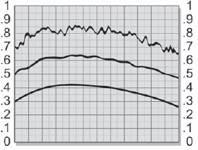
Figure 3-11: Smoothing Effects of Increasing the Blur Radius
The problem is that there is usually desirable matte edge detail that is at or near the same size as the grain we are trying to eliminate, so as the grain is eliminated so is our desirable detail. We therefore need the smallest blur radius that will attack the grain problem and leave the desirable detail.
3.3.3.2 The Blur Percentage
The second blur parameter, which I am calling the blur percentage, can be thought of as a “mix-back” percentage. It goes like this: Take an image and make a blurred copy. You now have two images: the original, and the blurred. Next, do a dissolve between the blurred image and the original image—say, a 50 percent dissolve. You are mixing back the original image 50 percent with the blurred image, hence a “mix-back” percentage. That's all there is to it. If your package does not offer a “percentage” parameter (by this or some other name) you now know how to make your own. Use a dissolve operation to create your own percentage parameter, as shown in Figure 3-12. It will add an extra node, but gives you an extra control knob over the strength of the blur, and control is the name of the game here.
If you do not have a dissolve operation, then scale the RGB values of the un-blurred version by (say) 30 percent and the blurred version by 70 percent, and then sum them together with an add node to make 100 percent. Changing the ratios (so they always total 100 percent, of course) allows any range of blur percentage.
3.3.4 Blurring Selected Regions
Even the minimum amount of blurring will sometimes destroy the fine detail in the matte edge. The only solution then is to perform a masked blurring operation that protects the regions with the fine detail from the blur operation. If the hair, for example, was getting blended away by the blurring operation, a mask could be created to hold off the blur from around the hair. The mask could be created either by hand (roto mask) or procedurally (chroma-key, as one example). Now the entire matte is blurred except for the hair region. There is another possibility. Rather than blurring the entire matte except for the holdout mask region, you might do the inverse by creating a mask that enables the blur in just one selected region. For example, let's say that composite tests have shown that the grain is objectionable only in the edges around a dark shirt. Create a mask for the dark shirt and enable the blur only in that region.
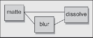
Figure 3-12: Creating Your Own Blur Percentage Feature
So your package does not support maskable blur operations? No problem. We'll make our own using a compositing substitute. Let's take the holdout mask for the hair as an example of the region we want to protect from a blur operation. First, make a blurred version of the entire matte. Then, using the hair mask, composite the unblurred version of the matte over the blurred version. The result is that the region within the hair mask is unblurred while the rest of the matte is blurred.
3.4 Adjusting the Matte Size
Very often the finished matte is “too large” around the perimeter, revealing dark edges around the finished composite. The fix here is to erode (shrink) the matte by moving the edges in toward the center. Many software packages have an “erode” (or shrink) and “expand” (or dilate) operation. Use ‘em if you got ‘em, but keep in mind that these edge processing nodes destroy edge detail, too. These nodes are edge processing operations that “walk” around the matte edge adding or subtracting pixels to expand or contract the region. These operations do retain the soft edge (rolloff) characteristics of the matte, but keep in mind that the edge details will still get lost. Figure 3-13 illustrates the progressive loss of edge detail with increasing matte erosion. Note especially the loss of the fine hair detail.
If you don't have these edge processing nodes, or they only move in unacceptably large integer (whole pixel) amounts, following are some work-arounds that may help. They show how to expand or contract a soft-edge matte with very fine control.
Figure 3-14 represents a finished matte that needs some refinement, either to expand or contract. The edge has been made very soft in order to make the results more visible. The following techniques show how to convert the gray edge pixels into either black transparency or white opacity regions, thus expanding or eroding the matte.
3.4.1 Shrinking the Matte with Blur and Scale
Figure 3-15 shows how to adjust the color curve to erode (shrink) the soft-edged matte shown in Figure 3-14 with the results shown in Figure 3-16. By pulling down on the blacks, the gray pixels that were part of the edge have become black and are now part of the black transparency region. By moving the color curve only slightly, very fine control over the matte edge can be achieved. The foreground region has shrunk, tucking the matte in all the way around the edges, but the edges have also become harder. If the harder edges are a problem, then go back to the original blur operation and increase it a bit. This will widen the edge transition region a bit more, giving you more room to shrink the matte and still leave some softness in the edge— at the expense of some loss of edge detail. Note the loss of detail in Figure 3-16 after the erode operation. The inner corners (crotches) are more rounded than in the original. This is why the minimum amount of this operation is applied to achieve the desired results.
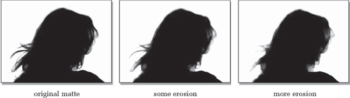
Figure 3-13: Progressive Loss of Edge Detail as the Matte Is Eroded


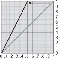
To see the difference between using an edge processing operation or the color curve tool to erode the matte, Figure 3-17 shows a slice graph of the edge of a soft matte that has been shifted by an edge processing operation. Note how the edge has moved inwards but has retained its slope, which indicates that the softness of the original edge was retained. Compared to Figure 3-18, the same edge was scaled with a color curve as described above. While the matte did shrink, it also increased its slope, and therefore its hardness increased. Normally, only small changes are required so the increase in edge hardness is usually not a problem. However, if an edge processing operation is available and offers the necessary fine control it is the best tool for the job.
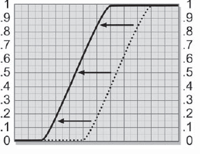
Figure 3-17: Erode by Edge Processing Operation
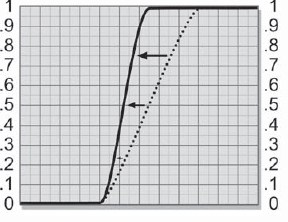
Figure 3-18: Erode by Scale Operation


3.4.2 Expanding the Matte with Blur and Scale
Figure 3-20 shows how to adjust the color curve to expand the soft-edged matte shown in Figure 3-19 (the same matte as in Figure 3-14), with the results shown in Figure 3-21. By pulling up on the whites, the gray pixels that were part of the inner edge have become white and are now part of the foreground white opacity region. The opaque region has expanded, and the edges have become harder. Again, if the harder edges are a problem, go back and increase the blur a bit. And yet again, watch for the loss of detail. Note how the star points are now more rounded than in the original.
The above operations were described as eroding and expanding the matte, but in fact they were actually eroding and expanding the whites, which happened to be the foreground matte color in this case. If you are dealing with black mattes instead, such as when pulling your own color difference mattes, then the color curve operations would simply be reversed or the matte inverted.