
CHAPTER 8
Action
Many shots are complete when the lightspace and camera attributes of the compositing layers match, but some shots will require you to match the action, or motion, as well. Motion tracking is one of the key tools for this, and is used to track one element onto another to create a match move. Yet another application of motion tracking is to stabilize a shot. Both of these processes and their variations are described in this chapter, along with some helpful tips, tricks, and techniques.
Geometric transformations, both 2D and 3D, are used to change the shape, size, and orientation of images as well as to animate them over time, as in the case of motion tracking. An understanding of the effects of pivot points and filter choices will protect you from degraded or unexpected results. The discussion of pivot points leads to some helpful techniques for the sometimes onerous task of lining one image up onto another. And as long as we are pushing images around, a discussion of image warps and morphs is in order.
8.1 Geometric Transformations
Geometric transformations are the processes of altering the size, position, shape, or orientation of an image. This might be required to resize or reposition an element to make it suitable for a shot, or to animate an element over time. Geometric transformations are also used after motion tracking to animate an element to stay locked onto a moving target as well as for shot stabilizing.
8.1.1 2D Transformations
2D transformations are called “2D” because they only alter the image in the X and Y planes, whereas the 3D transformations put the image into a three-dimensional world within which it can be manipulated. The 2D transformations—translation, rotation, scale, skew, and corner pinning—all bring with them hazards and artifacts. Understanding the sources of these artifacts and how to minimize them is an important component of all good composites.
8.1.1.1 Translation
Translation is the technical term for moving an image in X (horizontally) or Y (vertically), but may also be referred to as a pan or reposition by some less formal software packages. Figure 8-1 shows an example of a simple image pan from left to right, which simulates a camera panning from right to left.

Figure 8-1: Image Panning from Left to Right
Some software packages offer a “wraparound” option for their panning operations. The pixels that get pushed out of frame on one side will “wrap around” to be seen on the other side of the frame. One of the main uses of a wraparound feature is in a paint program. By blending away the seam in a wrapped-around image, a “tile” can be made that can be used repeatedly to seamlessly tile a region.
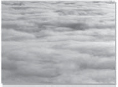
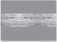
Figure 8-2 shows an original cloud image. In Figure 8-3 it has been panned in wraparound mode, which created a seam down the middle of the picture. The seam has been blended away in Figure 8-4, and the resulting image tiled three times horizontally in Figure 8-5. If you took the blended image in Figure 8-4, wrapped it around vertically, then painted out the horizontal seam, you would have an image that could be tiled infinitely both horizontally and vertically.
8.1.1.1.1 Floating Point versus Integer
You may find that your software offers two different pan operations, one that is integer and one that is floating point. The integer version may go by another name, such as “pixel shift.” The difference is that the integer version can position the image only on exact pixel boundaries, such as moving it by exactly 100 pixels in X. The floating point version, however, can move the image by any fractional amount, such as 100.731 pixels in X.
The integer version should never be used in animation because the picture will “hop” from pixel to pixel with a jerky motion. For animation, the floating point version is the only choice because it can move the picture smoothly at any speed to any position. The integer version, however, is the tool of choice if you need to simply reposition a plate to a new fixed location. The integer operation is not only much faster but it also will not soften the image with filtering operations as the floating point version will. The softening of images due to filtering is discussed in Section 8.1.3, “Filtering.”
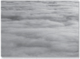
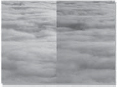
Figure 8-3: Wraparound Version
8.1.1.1.2 Source and Destination Movement
With some software packages you simply enter the amount to pan the image in X and Y and off it goes. We might call these absolute pan operations. Others have a source and destination type format, which is a relative pan operation. An example of a relative pan is shown in Figure 8-6. The relative pan operation is a bit more obtuse but can be more useful, as we will see in the image stabilizing and difference tracking operations. The source and destination values work by moving the point that is located at source X,Y to the position located at destination X,Y, dragging the whole image with it, of course. In the example in Figure 8-6, the point at source location 100, 200 will be moved to destination location 150, 300. This means that the image will move 50 pixels in X and 100 pixels in Y. It is also true that if the source were 1100, 1200 and the destination were 1150, 1300 it would still move 50 pixels in X and 100 pixels in Y. In other words, the image is moved the relative distance from the source to the destination. So what good is all this source and destination relative positioning stuff?
Suppose you wanted to move an image from point A to point B. With the absolute pan you have to do the arithmetic yourself to find how much to move the image. You will get out your calculator and subtract the X position of point A from the X position of point B to get the absolute movement in X, then subtract the Y position of point A from the Y position of point B to get the absolute movement in Y. You may now enter your numbers in the absolute pan node and move your picture. With the relative pan node, you simply enter the X and Y position of point A as the source, then the X and Y position of point B as the destination, and off you go. The computer does all the arithmetic, which, I believe, is why computers were invented in the first place.
8.1.1.2 Rotation
Rotation seems to be the only image processing operation in history to have been spared multiple names, so it will undoubtedly appear as rotation in your software. Most rotation operations are described in terms of degrees, so no discussion is needed here unless you would like to be reminded that 360 degrees makes a full circle. However, you may encounter a software package that refers to rotation in radians, a more sophisticated and elitist unit of rotation for the trigonometry enthusiast.
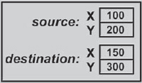
Figure 8-6: Source and Destination Type Pan
While very handy for calculating the length of an arc section on the perimeter of a circle, radians are not at all an intuitive form of angular measurement when the mission is to straighten up a tilted image. What you would probably really like to know is how big a radian is so that you can enter a plausible starting value and avoid whip-sawing the image around as you grope your way toward the desired angle. One radian is roughly 60 degrees. For somewhat greater precision, here is the official conversion between degrees and radians:
360 degrees = 2π radians (Eq. 8-1)
Not very helpful, was it? Although 2π radians might be equal to 360 degrees, you are still half a dozen calculator strokes away from any useful information. Here are a few precalculated reference points that you may actually find useful when confronted with a radian rotator.
| Radians to degrees | Degrees to radians |
| 1 radian ≅ 57.3 degrees | 10 degrees ≅ 0.17 radians |
| 0.1 radian ≅ 5.7 degrees | 90 degrees ≅ 1.57 radians |
At least now you know that if you want to tilt your picture by a couple of degrees it will be somewhere around 0.03 radians. Since 90 degrees is about 1.57 radians, then 180 degrees must be about 3.14 radians. You are now cleared to solo with radian rotators.
8.1.1.2.1 Pivot Points
Rotate operations have a pivot point, the point that is the center of the rotation operation. The location of the pivot point dramatically affects the results of the transformation, so it is important to know where it is, its effects on the rotation operation, and how to reposition it when necessary.
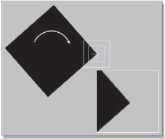
The rotated rectangle in Figure 8-7 has its pivot point in its center, so the results of the rotation are completely intuitive. In Figure 8-8, however, the pivot point is down in the lower right-hand corner and the results of the rotation operation are quite different. The degree of rotation is identical between the two rectangles, but the final position has been shifted up and to the right by comparison. Rotating an object around an off-center pivot point also displaces it in space. If the pivot point were placed far enough away from the rectangle it could actually rotate completely out of frame!
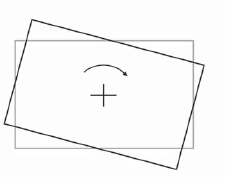
Figure 8-7: Centered Pivot Point
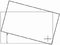
Figure 8-8: Off-Center Pivot Point
8.1.1.3 Scaling and Zooming
Scaling, resizing, and zooming are tragically interchangeable terms in many software packages. Regardless of the terminology, there are two possible ways that these operations can behave. A scale or resize operation most often means that the size of the image changes while the framing of the picture is unchanged, as in the examples in Figure 8-9.
A zoom most often means that the image size stays the same dimensions in X and Y, but the picture within it changes framing to become larger or smaller as though the camera were zoomed in or out, as in the example in Figure 8-10.
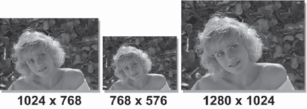
Figure 8-9: Image Scaling Operation: Image Size Changes but Framing Stays Constant
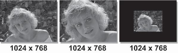
Figure 8-10: Image Zoom Operation: Image Size Stays Constant but Framing Changes
8.1.1.3.1 Pivot Points
The resize operation does not have a pivot point because it simply changes the dimensions of the image in X and Y. The scale and zoom operations, however, are like the rotation in that they must have a center about which the operation occurs. This is often referred to as the pivot point, or perhaps the center of scale, or maybe the center of zoom.
The scaled rectangle in Figure 8-11 has its pivot point in the center of the outline, so the results of the scale are unsurprising. In Figure 8-12, however, the pivot point is down in the lower right-hand corner, and the results of the scale operation are quite different. The amount of scale is identical with Figure 8-11, but the final position of the rectangle has been shifted down and to the right in comparison. Scaling an object around an off-center pivot point also displaces it in space. Again, if the pivot point were placed far enough away from an object it could actually scale itself completely out of the frame.
8.1.1.4 Skew
The overall shape of an image may also be deformed with a skew or shear, as in the examples in Figure 8-13. The skew shifts one edge of the image relative to its opposite edge—the top edge of the image relative to the bottom edge in a horizontal skew, or the left and right edges in a vertical skew. The skew normally does not have a pivot point because moving one edge relative to the other uses the opposite edge as the “center of action.” The skew is occasionally useful for deforming a matte or alpha channel to be used as a shadow on the ground, but corner pinning will give you more control over the shadow's shape and allow the introduction of perspective, as well.
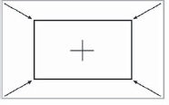
Figure 8-11: Centered Pivot Point

Figure 8-12: Off-Centered Pivot Point
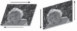
Figure 8-13: Horizontal and Vertical Skews
8.1.1.5 Corner Pinning
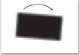
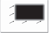
Corner pinning, shown in Figure 8-14, is an important image deformation tool because it allows you to arbitrarily alter the overall shape of an image. This is especially useful when the element you want to add to a shot isn't exactly the right shape or needs a subtle perspective shift. The image can be deformed as if it were mounted on a sheet of rubber where any or all of the four corners can be moved in any direction. The arrows in Figure 8-14 show the direction each corner point was moved in each example. The corner locations can also be animated over time so that the perspective change can follow a moving target in a motion tracking application.
Always keep in mind that corner pinning does not actually change the perspective in the image itself. The only way that the perspective can really be changed is to view the original scene from a different camera position. All corner pinning can do is deform the image plane the picture is on, which can appear as a fairly convincing perspective change, if it isn't pushed too far.
An example of a perspective change can be seen starting with Figure 8-15. The building was shot with a wide angle lens from a short distance away, so the picture has a noticeable perspective that tapers the building inward at the top. Figure 8-16 shows the taper taken out of the building by stretching the two top corners apart with corner pinning. The perspective change makes the building appear as though it were shot from a greater distance with a longer lens—unless you look closely, that is. There are still a few clues in the picture that reveal the close camera position if you know what to look for, but the casual observer won't notice them, especially if the picture is only on screen briefly.
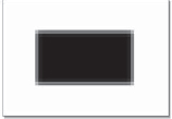
Another application of the perspective change is to lay an element on top of a flat surface, illustrated in Figures 8-17 through 8-20. The sign graphic in Figure 8-17 is to be added to the railroad car in Figure 8-18. The sign graphic has been deformed with four-corner pinning in Figure 8-19 to match the perspective. In Figure 8-20 the sign has been comped over the railroad car and now looks like it belongs in the scene. Most motion tracking software will also track four corners so that the camera or target surface can move during the shot. The corner pinned element will track on the target and change perspective over the length of the shot. This technique is most famously used to track a picture onto the screens of monitors and TV sets instead of trying to film them on the set.
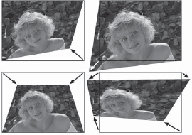
Figure 8-14: Corner Pinning Examples
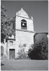
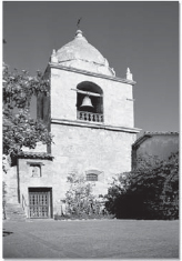
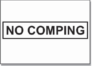
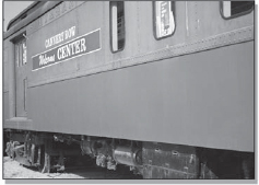
Figure 8-18: Original Background

Figure 8-19: Four-Corner Pinning to Create Perspective
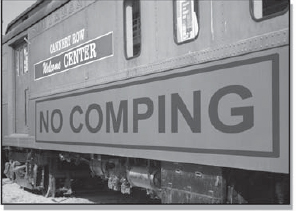
Figure 8-20: Perspective Graphic on Background
8.1.2 3D Transformations
3D transformations are so named because the image behaves as though it exists in three dimensions. You can think of it as though the picture were placed on a piece of cardboard. The cardboard can then be rotated and translated in any of the three dimensions and rendered with the new perspective. The traditional placement of the three-dimensional axes are shown in Figure 8-21. The X axis goes left to right, the Y axis up and down, and the Z axis is perpendicular to the screen, going into the picture.
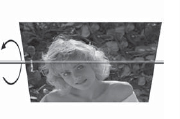
If an image is translated in X it will move left and right. If it is rotated in X (rotated about the X axis) it will rotate like the example in Figure 8-22. If the image is translated in Y it will move vertically. If it is rotated in Y it will rotate like the example in Figure 8-23. When translated in Z the image will get larger or smaller like a zoom as it moves toward or away from the camera. When rotated around Z (Figure 8-24) it rotates like a conventional 2D rotation. The 3D transformation node will have rotate, scale, and translate operations in the same node so that they can all be choreographed together with one set of motion curves.
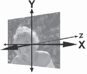
Figure 8-21: Three-Dimensional Axis


The time to use 3D transformations is when you want to “fly” something around the screen. Take a simple example like flying a logo in from the upper corner of the screen. The logo needs to translate from the corner of the screen to the center, and at the same time zoom from small to large. Coordinating these two movements so that they look natural together using conventional 2D scales and translations is tough. This is because the problem is in reality a three-dimensional problem and you are trying to fake it with separate two-dimensional tools. Better to use a 3D transformation node to perform a true 3D move on the logo.
8.1.3 Filtering
Whenever an image is transformed its pixels are re-sampled, or “filtered” to create the pixels for the new version of the image. These filtering operations can dramatically affect the results of a transformation, so an understanding of how they work and which ones to use under what circumstances can be very important.
8.1.3.1 The Effects of Filtering
In most cases, the filtering operation will soften the image because the new version is created by blending together percentages of adjacent pixels to create each new pixel. This is an irreversible degradation of the image. If you rotate an image a few degrees and then rotate it back, it will not return to its original sharpness.
An example can be seen starting with an extreme close-up of a small rectangular detail in the original image in Figure 8-25. It has a one-pixel border of anti-aliasing pixels at the outset. In Figure 8-26 the image has been rotated 5 degrees, and the re-sampled pixels can be seen all around the perimeter. Figure 8-27 illustrates a simple floating point translation of the original image and shows how the edge pixels have become blurred by the filtering operation. Of course, scaling an image up softens it even more because in addition to the filtering operation you have fewer pixels to spread out over more picture space.
A low-resolution image such as a frame of video will have sharp edges that are one pixel wide on most objects in the picture, while the sharp edges in a 2k resolution film frame naturally span several pixels. As a result, the effects of softening are much more noticeable on low-resolution images. If you have stacked up several transformations on an image and the softening becomes objectionable, see if you have a multifunction node that has all (or most) of the transformations in the one node. These nodes concatenate all of the different transformations (rotate, scale, translate) into a single operation, so the amount of softening is greatly reduced because the image is only filtered once.
Pixel shift operations do not soften the image because they do no filtering. The pixels are just picked up and placed into their new location without any processing, which is also why it is such a fast operation. Of course, as mentioned earlier, this makes it an integer operation, which should never be used for animation, but it is fine for the repositioning of a background plate.
The one case where filtering does not soften the image is when scaling an image down. Here the pixels are still being filtered, but they are also being squeezed down into a smaller image space, which tends to sharpen the whole picture. In film work, the scaled image could become so sharp that it actually needs to be softened to match the rest of the shot. This usually does not happen with video since the edges are normally one pixel wide already, and you can't get any sharper than that.
8.1.3.1.1 Twinkling Starfields
One situation where pixel filtering commonly causes problems is the “twinkling starfield” phenomenon. You've created a lovely starfield and then you go to animate it—either rotating it or perhaps panning it around—only to discover that the stars are twinkling! Their brightness is fluctuating during the move for some mysterious reason, and when the move stops, the twinkling stops.
What's happening is that the stars are very small, only 1 or 2 pixels in size, and when they are animated they become filtered with the surrounding black pixels. If a given star were to land on an exact pixel location, it might retain its original brightness. If it landed on the “crack” between two pixels it might be averaged across them and drop to 50 percent brightness on each pixel. The brightness of the star then fluctuates depending on where it lands each frame—it twinkles as it moves.
This is not to be confused with interlace flicker in video, although they can look similar. The distinction is that interlace flicker only shows up when the image is displayed on an interlaced video monitor, not the progressive scan monitors of most workstations. Another distinction is that interlace flicker persists even with a static image.
So what's the fix? Bigger stars, I'm afraid. The basic problem is that the stars are at or very near the size of a pixel, so they are badly hammered by the filtering operation. Make a starfield that is twice the size needed for the shot so that the stars are two or three pixels in diameter. Perform the rotation on the oversized starfield, then size it down for the shot. Stars that are several pixels in diameter are much more resistant to the effects of being filtered with the surrounding black.
The problem is exacerbated by the fact that the stars are very small, very bright, and surrounded by black—truly a worst-case scenario. Of course, this phenomenon is happening to your regular images, too; it's just that the effect is minimized by the fact that the picture content does not contain the extremes of high contrast and tiny features that are in a starfield.
8.1.3.2 Choosing a Filter
There are a variety of filters that have been developed for pixel re-sampling, each with its own virtues and vices. Some of the more common ones are listed here, but you should read your user guide to know what your software provides. The better software packages will allow you to choose the most appropriate filter for your transformation operations. The internal mathematical workings of the filters are not described because that is a ponderous and ultimately unhelpful topic for the compositor. Instead, the effects of the filter and its most appropriate application are offered.
Bicubic: High-quality filter for scaling images up. It actually incorporates an edge sharpening process so the scaled up image doesn't go soft so quickly. Under some conditions the edge sharpening operation can introduce “ringing” artifacts that degrade the results. Most appropriate use is scaling images up in size or zooming in.
Bilinear: Simple filter for scaling images up or down. Runs faster than the bicubic because it uses simpler math and has no edge sharpening. As a result, images get soft sooner. Best use is for scaling images down since it does not sharpen edges.
Impulse: A.k.a. “nearest neighbor,” a very fast, very low-quality filter. Not really a filter, it just “pixel plucks” from the source image—that is, it simply selects the nearest appropriate pixel from the source image to be used in the output image. Most appropriate use is for quickly making lower-resolution motion test of a shot. Also used to scale images up to give them a “pixelized” look.
Mitchell: A type of bicubic filter in which the filtering parameters have been refined for the best look on most images. Also does edge sharpening, but less prone to edge artifacts than a plain bicubic filter. Most appropriate use is to replace bicubic filter when it introduces edge artifacts.
Gaussian: Another high-quality filter for scaling images up. It does not have an edge enhancement process. As a result, the output images are not as sharp, but they also do not have any ringing artifacts. Most appropriate use is to substitute for the Mitchell filter when it introduces ringing artifacts.
Sinc: A special high-quality filter for downsizing images. Other filters tend to lose small details or introduce aliasing when scaling down. This filter retains small details with good anti-aliasing. Most appropriate use is for scaling images down or zooming out.
8.1.4 Lining Up Images
There are many occasions where you need to precisely line up one image on top of another. Most compositing packages offer some kind of “A/B” image comparison capability that can be helpful for lineup. Two images are loaded into a display window, then you can wipe or toggle between them to check and correct their alignment. This approach can be completely adequate for many situations, but there are times when you really want to see both images simultaneously rather than wiping or toggling between them.
The problem becomes trying to see what you are doing, because one layer covers the other. A simple 50 percent dissolve between the two layers is hopelessly confusing to look at, and overlaying the layers while wiping between them with one hand while you nudge their positions with the other is slow and awkward. What is really needed is some way of displaying both images simultaneously that still keeps them visually distinguished while you nudge them into position. Two different lineup display methods are offered here that will help you to do just that.
8.1.4.1 Offset Mask Lineup Display
The offset mask method combines a monochrome version of two images in such a way that if the two images are not perfectly aligned an embossed outline shows up, as in the example in Figure 8-28. The embossing marks all pixels that are not identical between the two images. If they are exactly lined up on each other the embossing disappears and it becomes a featureless gray picture.
To make the lineup mask, a monochrome version is first made of the two images to be lined up. One of the mono images is scaled down in brightness by 50 percent and the other is first inverted (in brightness, of course), then also scaled down in brightness by 50 percent. It does not matter which image is the inverted one. The two 50 percent brightness versions are then simply added together. A pictographic flowgraph of the whole process is shown in Figure 8-29. A good way to familiarize yourself with this procedure is to use the same image for both input images until you are comfortable that you have it set up right and can “read” the signs of mis-alignment. Once set up correctly, substitute the real image to be lined up for one of the inputs.

Figure 8-28: Embossed Effect from Offset Images
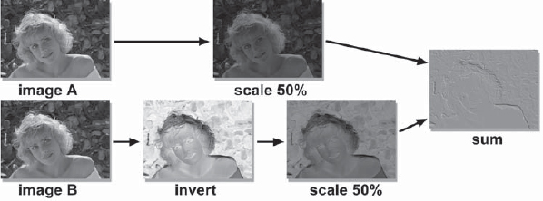
Figure 8-29: Pictographic Flowgraph of the Offset Mask Lineup Procedure
Once set up, the procedure is to simply reposition one of the images until the offset mask becomes a smooth gray in the region you want lined up. This is a very precise “offset detector” that will reveal the slightest difference between the two images, but it suffers from the drawback that it does not tell you directly which way to move which image to line them up. It simply indicates that they are not perfectly aligned. Of course, you can experimentally slide the image in one direction, and if the embossing gets worse, go back the other way. With a little practice you should be able to stay clear on which image is which.
8.1.4.2 Edge Detection Lineup Display
Lineup method number two is the edge detection method. The beauty of this method is that it makes it perfectly clear which image to move in which direction to achieve the lineup. The basic idea is to use an edge detection operation on a monochrome version of the two images to make an “outline” version of each image. One image is placed in the red channel, the other in the green channel, and the blue channel is filled with black, as shown in the flowgraph in Figure 8-30. When the red and green outline images are correctly lined up on each other, the lines turn yellow. If they slide off from each other, you see red lines and green lines again, which tell you exactly how far and in what direction to move in order to line them up.
Examples of this lineup method can be seen in Color Plate 61 through Color Plate 64. They show the monochrome image and its edge detection version, then how the colors change when the edges are unaligned (Color Plate 63) versus aligned (Color Plate 64).
One of the difficulties of an image lineup procedure is trying to stay clear in your mind as to which image is being moved and in what direction. You have an image being repositioned (the repo image) and a target image that you are trying to line it up to. If you put the target image in the red channel and the repo image in the green channel as in the example in Figure 8-30, then you can just remember the little mnemonic—”move the green to the red.” Since the color green is associated with “go” and the color red with “stop” for traffic lights, it is easy to stay clear on what is being moved (green) versus what is the static target (red). While this method makes it easier to see what you are doing, it is sometimes less precise than the offset mask method.
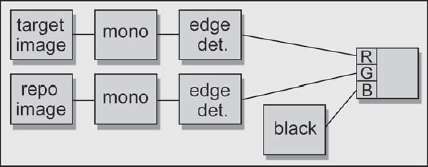
Figure 8-30: Flowgraph of Lineup Edges
8.1.4.3 The Pivot Point Lineup Procedure
Now that we have a couple of good ways to see what we are doing when we want to line up two images, this is a good time to discuss an efficient method of achieving the actual lineup itself. The effects of the pivot point location can be used to excellent advantage when trying to line up two elements that are dissimilar in size, position, and orientation. It can take quite a bit of trial and error in scaling, positioning, rotating, repositioning, rescaling, repositioning, and so on, to get two elements lined up. By using a strategically placed pivot point and a specific procedure, however, a complex lineup can be done without all of the trial and error. Here's how.
The mission: Line up the smaller, dark, four-point star with the larger gray star. The smaller star is out of position, rotated, and scaled differently in X and Y compared to the target star. Select a point that the two objects have in common to use as the pivot point. For this demo the lower left-hand corner will be the common point.

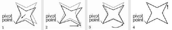
Step 1: Reposition the element so that its common point is on top of the target's common point. Set this common point as the pivot point for all subsequent operations.
Step 2: Scale the element in X from the pivot point until its right edge aligns with the target.
Step 3: Rotate the element around the pivot point to orient it with the target.
Step 4: Scale the element in Y from the pivot point until its top edge aligns with the target. Done. Take a break.
8.2 Motion Tracking
Motion tracking is one of the most magical things that computers can do with pictures. With relentless accuracy and repeatability, the computer can track one object on top of another with remarkable smoothness or stabilize a bouncy shot to rock-solid steadiness. The reason to stabilize a shot is self-evident, but the uses of motion tracking are infinitely varied. An element can be added to a shot that moves convincingly with another element and even follows a camera move, or, conversely, an element in the scene can be removed by tracking a piece of the background over it.
Motion tracking starts by finding the track, or the path of a target object in the picture. This track data is then used to either remove the motion from a shot in the case of stabilizing, or to add motion to a static element so it will travel with the target object. It is the same tracking data, but it can be applied two different ways. There are even variations in the applications, such as smoothing the motion of a shot rather than totally stabilizing it, and difference tracking, where one moving object is tracked over another moving object.
8.2.1 The Tracking Operation
Motion tracking is a two-step process. The first step is the actual tracking of the target object in the frame, which is a data collection operation only. Later, the tracking data will be converted into motion data. This motion data may take the form of stabilizing the shot or tracking a new element onto a moving target in a background plate. Most compositing software will track the entire shot first, then export all of the motion data to some kind of motion node to be used in a subsequent render. Some systems, like Flame, track and export motion data one frame at a time so that you can watch it stabilize or track as it goes, but this is an implementation detail and not a fundamental difference in the process.
The first operation is to plant tracking points on key parts of the picture, which serve as the tracking targets, like those in Figure 8-31. The computer will then step through all of the frames in the shot, moving the tracking points in each frame to keep them locked onto the tracking targets. This is the data collection phase, so collecting good tracking data is obviously a prerequisite to a good motion track.
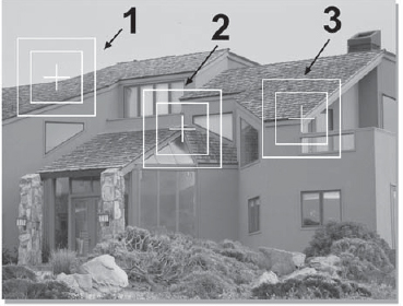
Figure 8-31: Tracking Points on Tracking Targets
You may have noticed that the tracking points in Figure 8-31 are surrounded by two boxes. The inner box is the match box. It is the pixels within this box that are analyzed for a match. The outer box is the search box, and it defines the area the computer will search looking for a match in each frame. The larger these boxes are the more computing time will be required for each frame, so they need to be as small as possible. If the motion in the frame is large, the search box must also be large because the target will have moved a lot between frames and the target needs to stay within the search box in each frame to be found. The larger the target, the larger the match box must be, so hopefully your shots will have small targets that move slowly. Motion tracking can become a time-consuming process.
The actual algorithms vary, but the approach is the same for all motion trackers. On the first frame of the tracking, the pixels inside the match box are set aside as the match reference. On the second frame, the match box is repeatedly repositioned within the bounds of the search box and the pixels within it compared to the match reference. At each match box position a correlation routine calculates and saves a correlation number that represents how closely those pixels match the reference.
After the match box has covered the entire search box, the accumulated correlation numbers are examined to find which match box position had the highest correlation number. If the highest correlation number is greater than the minimum required correlation (preferably selectable by you), we have a match and the computer moves on to the next frame. If no match is found, most systems will halt and complain that they are lost and could you please help them find the target. After you help it find the target, the automatic tracking resumes until it gets lost again, or the shot ends, or you shoot the computer (this can be frustrating work).
8.2.1.1 Selecting Good Tracking Targets
One of the most important issues at the tracking stage is the selection of appropriate tracking targets. Some things do not work well as tracking targets. Most tracking algorithms work by following the edge contrasts in the picture, so high-contrast edges are preferred. The second thing is that the tracking target needs good edges in both X and Y. In Figure 8-31 tracking points #2 and #3 are over targets with good edges in both directions, but point #1 is not. The problem for the tracker becomes trying to tell if the match box has slipped left or right on the roof edge since there are no good vertical edges to lock onto. Circular objects (light bulbs, door knobs, etc.) make good tracking targets because they have nice edges both horizontally and vertically.
A second issue is to select tracking targets that are as close as possible to the locking point, the point in the picture that you wish the tracked item to lock to. Take the fountain in Figure 8-32, for example. Let's say that you want to track someone sitting on the fountain wall at the locking point indicated and the shot has a camera move. There are potential tracking points all over the frame, but the camera move will cause the other points in the picture to shift relative to the locking point, and for a variety of reasons.
If the camera's position is moved with a truck, dolly, or boom there will be noticeable parallax shifts in the shot that cause points in the foreground to move differently from those in the background. However, even if the camera is just panned or tilted, there can still be subtle parallax shifts between points in the foreground and background.
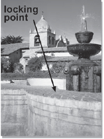
Figure 8-32: The Locking Point
Another variable is lens distortion. As the different tracking points move through the lens's distortion field at different times, their relative positions shift in the picture. The problem with these problems is that they often are not perceptible to the eye. They are, of course, perfectly obvious to the computer. All of these subtle positional shifts introduce errors into the tracking data, which will result in the tracked object “squirming” around the locking point instead of being neatly locked to it. So make sure that you select tracking points that are as close as possible to the locking point.
8.2.1.2 Enable/Disable Tracking Points
The tracking targets are frequently not conveniently on screen for the full length of the shot. The tracking target may move out of frame or something may pass in front of it, blocking it from view for a few frames. To accommodate this, any motion tracker worth its weight in pixels will have an enable/disable feature for each tracking point. If the target for tracking point #3 goes away on frame 100, that point must be disabled on frame 100. Should the target be blocked for 10 frames, it is disabled for those 10 frames. Later, during the calculation phase, the computer will ignore the tracking point while it was disabled and use only the enabled points for its calculations.
8.2.1.3 Keep Shape and Follow Shape
Using the pixels from the first frame of the motion track as the match reference for all subsequent frames works fine if the tracking target maintains the same shape over the entire length of the shot. But what if it doesn't?
Figure 8-33 illustrates a fine tracking target, the corner of a square. It has strong vertical and horizontal edges, and the match reference that it creates on the first frame of tracking is shown in the inset. But this particular square rotates. Figure 8-34 shows the same square several frames later, and the inset shows what the match box sees then. This will correlate very poorly with the match reference made from the first frame, so the system declares “no match” and halts.
The solution to this class of problem is to have the system follow the changing shape of the target in each frame by using the previous frame's best match as a new match reference. The target probably will not have changed very much between two adjacent frames. So the best match of frame 51 becomes the match reference for frame 52, and so on. Creating a new match reference each frame to follow a target that is constantly changing shape is called by some a follow shape mode. Keeping the same shape as the match reference over the entire shot is called by some a keep shape mode. Your software may have different names, of course.
You really want your software to allow you to select which mode to use, keep shape or follow shape, as well as switch between them when appropriate. The reason is that while the follow shape mode solves the problem of a tracking target that changes shape, it introduces a new problem of its own. It produces much poorer tracking data. This is because each frame's match is based on the previous frame, so small match errors accumulate over the entire length of the shot. With keep shape, each frame is compared to the same match reference, so while each frame has its own small match error, the errors do not accumulate.
My favorite metaphor for describing the errors between the keep shape and follow shape modes is to offer you two methods of measuring a long, 90-foot hallway. With the keep shape method you get to use a 100-foot measuring tape. While you may introduce a small measuring error because you did not hold the tape just right, you only have the one error. With the follow shape method you have to use a 6-inch ruler. To measure the 90-foot hallway you must crawl along the floor repositioning the ruler 180 times. Each time you place the ruler down you introduce a small error. By the time you get to the end of the hall you have accumulated 180 errors in measurement, and your results are much less accurate than with the single 100-foot tape measure. So the rule is, use keep shape whenever possible and switch to follow shape only on those frames where keep shape fails.
8.2.2 Applying the Tracking Data
Once the tracking data is collected, the second step in motion tracking is to apply it to generating some kind of motion (except for Flame, which applies as it goes). Once collected, the tracking data can be interpreted in a variety of ways, depending on the application. From the raw tracking data the computer can derive the motion of a pan, rotate, or scale (zoom), as well as four-point corner pinning (hopefully). The tracking data can also be applied in two different ways. Applied as tracking data, it tracks a static object on top of a moving target, matching movement, rotation, and size changes. Applied as stabilization data, it removes the movement, rotation, and zoom changes from each frame of a shot to hold it steady.
Multiple tracking points have been laid down, some enabled and disabled at various times, and all of this data needs to be combined and interpreted to determine the final track. Why interpreted? Because there are irregularities in the raw tracking data and some sort of filtering and averaging must always be done.
To take even a simple case such as tracking a camera pan, in theory, all of the tracking points will have moved as a fixed constellation of points across the screen. Determining the pan from such data should be trivial. Just average together all of their locations on a frame-by-frame basis and consolidate that to a single positional offset for each frame. In practice, the tracking points do not move as a fixed constellation but have jitter due to grain plus squirm due to lens distortions and parallax. The calculation phase, then, has rules that differ from software to software on how to deal with these issues to derive a single averaged motion, rotation, and scale for each frame.
The results of the tracking calculations are relative movements, not actual screen locations. The tracking data actually says “from wherever the starting location is, on the second frame it moved this much relative to that location, on the third frame it moved this much, on the fourth frame . . . etc.” Because the tracking data is relative movement from the starting position there is no tracking data for the first frame. The tracking data actually starts on the second frame.
To take a concrete example, let's say that you have tracked a shot for a simple pan. You then place the object to be tracked in its starting location on the screen for frame one, and on frame two the tracking data will move it 1.3 pixels in X and 0.9 pixels in Y relative to its starting location. This is why it is important that the tracking points you place be as close as possible to the actual locking point. Tracking data collected from the top half of the screen but applied to an object that is to lock to something on the bottom half of the screen will invariably squirm.
8.2.3 Stabilizing
Stabilizing is the other grand application of motion tracking, and it simply interprets the same motion tracking data in a different way to remove the camera motion from the shot. If the tracking data is smoothed in some way, either by hand or by filters, the bouncy camera move can be replaced by a smooth one that still retains the basic camera move. One thing to keep in mind about stabilizing a shot, however, is the camera motion blur. As the camera bounced during the filming it imparted motion blur to some frames of the film. When the shot is stabilized, the motion blur will remain, and in extreme cases it can be quite objectionable.
After the tracking data is collected, it is interpreted and then exported to an appropriate motion node to back out all of the picture movement relative to the first frame. All subsequent frames align with the first frame to hold the entire shot steady. This section addresses some of the problems this process introduces and describes ways to trick your software into doing motion smoothing rather than total stabilizing, which is often a more appropriate solution to the problem for a couple of reasons.
8.2.3.1 The Repo Problem
When a shot is stabilized, each frame is repositioned in order to hold the picture steady. This introduces a serious problem. As the frames are repositioned, the edges of the picture move into frame, leaving a (usually) black margin where the picture used to be. Let's say that we want to stabilize the sequence of bouncy camera frames in Figure 8-35 by locking onto the tower and holding it steady relative to frame one. The stabilized version of the same sequence is shown in Figure 8-36 with the resulting severe black reposition margins.
Frame 1 in Figure 8-36, being the first frame in the stabilized sequence, was not repositioned because it is the reference frame to which all of the others are locked. Frames 2 and 3 in Figure 8-36 have been repositioned to line up with frame 1, and as a result they have severe black margins. The fix for this is to zoom into each frame by scaling it up after it has been repositioned such that the black margins are pushed out of frame. This means that the scale factor must be large enough to clear the black margin out of the worst-case frame.
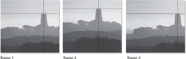
Figure 8-35: Original Frames with Tracking Target
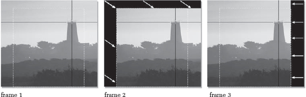
Figure 8-36: Stabilized Frames
The stabilized frames in Figure 8-36 have a dotted outline that represents the “lowest common denominator” of useable area that will remain after the scale operation. But zooming into pictures both softens and crops them. Therefore, as an unavoidable consequence of the stabilizing process, to some degree the resulting stabilized shot will be both zoomed in and softened compared to the original. Very often the client is unaware of this, so a little client briefing before any work is done might save you some grief later.
8.2.3.2 Motion Smoothing
Motion smoothing helps to minimize the two problems introduced from stabilizing a shot, the push-in and the residual motion blur. While the push-in and softening from stabilizing are inherently unavoidable, they can be minimized by reducing the excursions. The excursion is the distance each frame has to be moved to stabilize it, and the amount of scaling that is required is dictated by the maximum excursions in X and Y. Reducing the maximum excursion will reduce the amount of scaling, and the maximum excursion can be reduced by reducing the degree of stabilization. In other words, rather than totally stabilizing the shot, motion smoothing may suffice. Since some of the original camera motion is retained with motion smoothing, any motion blur due to camera movement will look a bit more natural than it does in a totally stabilized shot.
To apply this to a practical example, if a bouncy shot has to be locked down to rock steady, the excursions will be at their maximum. If the bouncy camera motion can be replaced with an acceptably gentle moving camera instead, the maximum excursion can be greatly reduced, so the amount of push-in and softening will also be greatly reduced. The following procedure is based on the use of a pan, or translate node, that has source and destination motion curves, as described in Section 8.1.1.1, “Translation.”
While presented here as a possible solution to excessive scaling in a stabilized shot, this motion smoothing procedure can also be applied to any wobbly camera move to take out the wobble but retain the overall camera move.
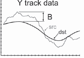
To simplify our story, we will assume a shot has been tracked that only has vertical jitter, so we are only concerned with the Y track data shown in Figure 8-37. The raw track data represents how much the tracking target was displaced on each frame, and is drawn as the light gray curve labeled “src” (source). It is called the source because to stabilize a frame it must be moved from its source position to its destination position. The destination position is marked with the flat line labeled “dst,” which is a flat line because to totally stabilize the shot the tracking target must be moved vertically to the exact same position each frame. The maximum excursion is labeled “A” and represents the greatest distance that the picture will have to be repositioned to stabilize it.
Figure 8-38 represents a motion-smoothed version of the same Y track data. Instead of totally locking the shot off, this approach allows the camera to gently sway up and down, reducing the jittery camera to an acceptably smooth camera move. The maximum excursion, labeled “B,” is dramatically reduced compared to the totally stabilized shot in Figure 8-37. It will now require less than half as much scaling to clear the black margins out of the frame, which will dramatically reduce the push-in and softening compared to the totally stabilized version.

Figure 8-37: Totally Stabilized
Now the question becomes how to do this with your particular software. With some software the motion tracker is a closed “black box” which does not permit you to get creative. If there is a motion smoothing option, you're in luck. If not, there is nothing you can do until you upgrade. Other software will allow you to export the motion tracking data to other nodes that do the actual pan, rotate, and scale operations. These we can get creative with.
The basic idea is to export the tracking data to a pan (translate) node so that it ends up in a source motion channel, then create a smoothed curve in the destination motion channel, as in Figure 8-38. There are two ways the smoothed curve might be created. If your software has curve smoothing functions, the choppy source channel can be copied into the destination channel, then smoothed. The second approach is to simply draw a new, smooth curve by hand in the destination channel. The pan node will then move each frame just the small distance from the source position to the destination position to smooth the motion. Be sure to export the data as track data, as though you wanted to track an object to the picture. This way the actual motion of the target point is placed in the source motion channel. If the track data is exported as stabilize data it will be inverted to remove all motion from the shot, which we do not want.
8.2.4 3D Motion Tracking
There is an even more sophisticated form of motion tracking, and that is 3D motion tracking, sometime referred to as a “match move.” The purpose of this type of motion tracking is to derive the actual three-dimensional camera move in a shot, then transfer that camera data to a 3D animation package so that a matching camera move can be added to a cgi element that is to be composited into the scene. Since this is in actuality a cgi application, it is outside the scope of this book. However, a brief overview of the process might be interesting and informative and lend a few insights to 2D tracking situations, as well.
There are three main requirements for 3D motion tracking: camera lens information, measurements from the set, and good tracking markers. The lens information is required by the analysis software that is trying to discover the camera position, because the lens distorts the true position of the tracking markers and its effects have to be backed out of the calculations. A survey of the set to collect some reliable measurements is essential for the tracking software to have at least some solid references to work with. The analysis process entails a “best fit” approach, so having at least a few reliable numbers to use as starting assumptions is essential.
Figure 8-39 shows an interior set with many convenient tracking points circled. The nature of the set provides several handy corners and small objects that make good tracking targets. This shot could be tracked as is using just measurements surveyed from the set. However, many scenes do not have good tracking targets naturally, so tracking markers are often added, then painted out later.
Because greenscreen shots by definition have large, featureless regions that provide no useful tracking points, they often have to be added. Figure 8-40 shows the typical tracking markers (the crosses on the bluescreen) added to a bluecreen shot. The markers can simply be a contrasting colored masking tape with measurements taken of their locations. Of course, bluescreen shots sometimes require 2D tracking, so these same tracking markers will serve there as well.
Large, exterior shots provide a different set of challenges to the match move department. They often have very large, sweeping camera moves using booms, trucks, helicopters, cable-cams, and even hand-held steadicams, or—my personal favorite— hand-held unsteady cams. Broad, open spaces such as fields may also be fairly featureless, and any useable natural tracking points might be difficult to measure and inappropriately located. Here, too, tracking markers might have to be added and measured, as shown in Figure 8-41. These tracking markers will typically be spherical so that they provide a constant shape to the tracker from any camera angle.
Two-dimensional tracking might be done with just three or four points, but 3D tracking requires many more. In fact, the more points that can be tracked, the more accurate the resulting camera move data will be. It is not uncommon to track 20 to 50 points in these cases. The tracking software is also more sophisticated and difficult to operate, requiring much intervention from the operator to give it “hints” and “clues” as to where the camera must be (no, it is not below the ground looking up at the scene!) and when to discard confusing tracking points. There is also great variability between 3D tracking software packages in the speed and accuracy of their results. However, there simply is no other way to create a cgi element with a matching camera move to the live action scene, a requirement being demanded by more and more directors who disdain locked off camera shots.

Figure 8-39: 3D Tracking Points

Figure 8-40: Bluescreen Tracking Markers

Figure 8-41: Exterior Tracking Markers
8.2.5 Tips and Techniques
When theory meets practice, reality steps in to muddle the results. In this section some of the problems that are often encountered with motion tracking are described, along with some tips and techniques on how to deal with them.
8.2.5.1 Tracking Preview
Before you start motion tracking a shot, make a low-resolution preview of the shot that you can play in real time. Look for good tracking targets and note when they go out of frame or are occluded. Watch for any parallax in the scene that will disqualify otherwise attractive tracking targets. Having a well-thought-out plan of attack before you begin placing any tracking points will save you time and trouble when you go to do the actual motion tracking.
8.2.5.2 Low-Resolution/High-Resolution Tracking
Some motion trackers will allow you to track a shot at low resolution (low res) with proxies, then switch to the high-resolution images later. Software that permits this is a very big time-saver when you are working with high-resolution film frames (the savings are minimal with video resolution frames). The basic idea is to set up the motion track on the low-res proxies, then retrack on the high-res frames after you get a clean track at low res.
Tracking the shot with low res proxies first provides two big advantages. The first is that the tracking goes much faster, so problems can be found and fixed that much more quickly. The second advantage is that any tracking target that the tracker can lock onto at low res it can lock onto even better at high res because of the increased detail. This means that when you switch to high res and retrack the shot it should track the entire shot the first time through without a hitch. All of the tracking problems have been found and fixed at low res, which is much faster than slugging through the high res tracking several times trying to get a clean track.
A related suggestion, again for high-res film frames, is that it will often suffice to track the shot at half res, then apply the half-res tracking data to the high-res frames. In other words, motion tracked data from the half-res proxies is often sufficiently accurate for the full-res frames, so it is often not necessary to do the actual tracking at high res. This assumes that your motion tracker is “resolution independent” and understands how to appropriately scale all of the motion data when you switch from half res to full res.
8.2.5.3 Preprocessing the Shot
Problems can arise in the tracking phase from a number of directions. The tracking targets may be hard to lock on to, you may get a jittery track due to film grain, and you might have squirm in your tracked motion due to lens effects. There are a number of things you can do to preprocess the shot and help the hapless motion tracker do a better job.
8.2.5.3.1 Increase the Contrast
One of the most annoying problems is the motion tracker losing the tracking target, even when it is right in plain view. Assuming the problem is not simply that the target is outside of its search box so that it just can't find it, there may not be enough contrast in the picture for it to get a good lock. Make a high-contrast version of the shot and use it for the tracking. Many motion trackers just look at the luminance of the image anyway and don't actually look at the color of the pixels. Perhaps a high-contrast grayscale version would be easier for the tracker to lock onto, or perhaps just the green channel would make a better target. Beware of going too far in slamming the contrast, however. This will harden the target's edge pixels, making them chatter. The resulting track would then jitter as it attempted to follow a chattering edge. Not good.
8.2.5.3.2 Degrain
Speaking of jittery tracks, film grain can also give you jittery tracks. High-speed films have very big grain that creates a “dancing target” for the tracker, resulting in the jittery motion track. Increasing the contrast will increase the problem. There are a couple of approaches. You can degrain the picture, or, if you don't have a degrain operation, a gentle blur might do. Another approach is to get rid of the blue channel, which has the most grain. Copy the red or green channel into the blue channel to create a less grainy version of the image to track with, or make a monochrome version by averaging the red and green channels together.
8.2.5.3.3 Lens Distortion
Lens distortion is another cause of motion tracking problems. Lens distortions will result in the tracked item squirming around its locking point. The reason for this can be seen in Figure 8-42, which shows the distortion map of a representative lens. As the camera pans to the right, you would expect points 1 and 2 to both move to the left in a perfectly straight horizontal path and at the same speed. However, point 2 moves in an arc and also changes speed relative to point 1. The two points drift both left and right as well as up and down relative to each other. (With a theoretically perfect lens the two points would stay locked together at the same distance apart as they moved.) When the time comes to calculate the actual camera pan from these two points, the averaging of their positions will cause the calculated locking point to drift around, which introduces the squirm into the tracking data.
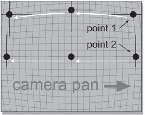
Figure 8-42: Effects of Lens Distortion on Tracking Points
The preprocessing fix for this lens distortion is to undistort the entire shot to make the picture flat again. The tracking and compositing are then done on the flat version, and the finished results then warped back to the original shape, if desired. While difficult to do, it can be done with any image warping package. Clearly this is only worth the effort if the lens distortions are wreaking havoc with your motion track. If there is a zoom in the shot the lens distortions may change over the length of the shot, rendering the problem that much more difficult.
You would think that someone could write a program where you could just enter “50mm lens” and it would back out the lens distortions. Alas, this is not even in the cards. Not only do you often not know what the lens is, but each manufacturer's 50mm lens will have a different distortion, and there are even variations from lens to lens of the same manufacturer! The most effective method is to film a grid chart with the actual lens used in the shot and use that to make a distortion map.
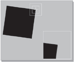
8.2.5.4 Point Stacking
In general, the more points you track on a shot the better the resulting tracking data will be. This is because the various tracking points will be averaged together later to derive the “true” track of the target, and the more samples that are averaged together the more accurate the results. However, what if there are not five or six convenient tracking targets in frame for the whole shot? What if there are only one or two potential tracking targets in the shot? The answer is point stacking, of course. You can paste several tracking points on top of each other over the same target, as in Figure 8-43. The computer does not know that they overlap or that they are on the same target. You get valid tracking data from each point, just as though they were spread all over the screen.
One key point, however, is that the tracking points must not be stacked exactly on top of each other. If they are, they will all collect the same tracking data, which is no better than one tracking point. But by having them slightly offset from each other like the three tracking points in Figure 8-43, each match box generates a slightly different sample of the image for the correlation routine. All three tracking points will eventually be averaged together to create a single, more accurate track.
8.2.5.5 Difference Tracking
Motion tracking is used most often to track a stationary object onto a moving target. However, there are times when you have a moving object to track onto a moving target. This is where difference tracking comes in. You want to track the difference between the moving object and the moving target. This technique requires the source and destination type motion nodes described in Section 8.1.1.1, “Translation.” For a simplified example, we will assume that the only motion to be tracked is translations in X and Y, so that a pan node will suffice.
The basic idea is to perform tracking operations on both the moving object and the moving target, then combine their motion data in a single difference pan node that will keep the moving object tracked on the moving target. The motion curves in Figure 8-44, Figure 8-45, and Figure 8-46 represent generic motion channels within the pan nodes. Following are the specific steps:
Step 1: Track the moving object, and then export its track data to pan node #1 (Figure 8-44).
Step 2: Track the moving target, and then export its track data to pan node #2 (Figure 8-45).
Step 3: Copy the moving object's motion data from pan node #1 to the source channels of pan node #3 (Figure 8-46).
Step 4: Copy the moving target's motion data from pan node #2 to the destination channels of pan node #3 (Figure 8-46).
Step 5: Connect pan node #3 to the moving object image for the composite over the target image (Figure 8-47).
Step 6: Reposition the moving object to its desired starting position by shifting the source channel motion curves in pan node #3.
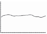
Figure 8-44: Pan Node #1 Object Motion Track
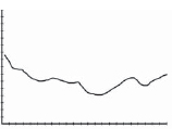
Figure 8-45: Pan Node #2 Target Motion Track
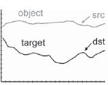
Figure 8-46: Pan Node #3 Difference Track
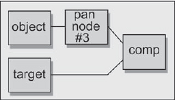
Figure 8-47: Flowgraph of Difference Track
Pan node #3 (the difference tracking node) now has the motion track of the moving object in its source channels and the motion track of the moving target in its destination channels. Recalling that the source and destination position channels mean “move the image from the source position to the destination position,” pan node #3 will move the moving object position to the moving target position for each frame.
This assumes that the moving object starts in the correct position, which was the purpose of Step 6. Selecting the entire source X motion channel and shifting it up and down in the curve editor will shift the starting position of the moving object left and right. Similarly, shifting the source Y motion channel up and down will shift the starting position vertically.
If your software does not support some of the operations required for this procedure, there is a fallback procedure. You could first stabilize the moving object, then track the stabilized version onto the moving target. This is less elegant and performs two transformations which increases the rendering time and degrades the image by filtering it twice rather than once, but you may have no choice in the matter.
8.3 Warps and Morphs
The image warp is another one of those magical effects that only computers can do. Only a few compositing packages contain image warping tools, so this operation is often done using a dedicated external software package, then importing the warped images or the morph into the main compositing package. Although the image warp is occasionally used to reshape an element so that it will physically fit into a scene, the most common application of warps is to produce a morph.
8.3.1 Warps
Warps are used to perform nonlinear deformations on images. That is to say, instead of a simple linear (equal amount everywhere) operation such as scaling an image in X, this process allows local deformations of small regions within the image. The corner pinning operation described in Section 8.1.4 is a global operation—the corner is repositioned and the entire image is deformed accordingly. With warps, just the region of interest is deformed.
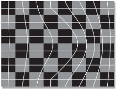
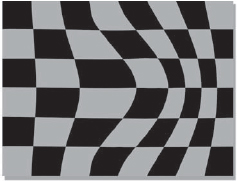
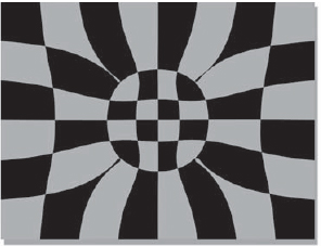
One of the earliest and simplest warp methodologies is the mesh warp, illustrated in Figure 8-48 and Figure 8-49. The mesh is a two-dimensional grid superimposed over the image. The intersections are points that can be moved around to describe the desired deformation, and the connections between the points are a spline. If a straight line were used between the mesh points the resulting warped image would also have straight section deformations. The splines guarantee gracefully curved deformations that blend naturally from point to point. You basically move the mesh points around to tell the machine how you want to deform the image, then the computer uses your mesh to render the warped version of the image.
A mesh warper is easy to design and use, but difficult to control. You don't have control points exactly where you want them, and it is hard to correlate the warped image to its intended target shape. Their most appropriate use is “procedural” warping effects such as lens distortions, pond ripples, flag waving, and so forth.
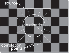
A spline warper is the “second generation” of warpers and works on entirely different principles. It offers much more control over the warp and excellent correlation to the target image, and is accordingly more complicated to learn and use. Think of a warp as the movement of different regions of the picture from one location to another. There must not only be a way to describe those regions to the computer, but also their final destinations. This is done with the source and destination splines along with their correlation points.
The operator (that's you) draws an arbitrary shape on the image that represents the source, or start position of the warp, represented by the square in Figure 8-50. This line means “grab the pixels here.” The operator then draws a second arbitrary shape, the destination, represented by the circle, which means “move those pixels to here.” In this particular example we are warping a square region into a circular one. After the source and destination splines are set the operator must then establish the “correlation” between them, which describes their connectivity. This tells the computer which regions of the source spline go to which regions of the destination spline. These connections are indicated by the correlation points, the dotted lines in Figure 8-50. This arrangement provides unambiguous instructions to the computer as to which regions of the image you want moved to what destinations in order to create the warp you want.
One of the very big advantages of spline warpers is that you can place as many splines as you want in any location you want. This allows you to get lots of control points exactly where you want them for fine detail work. The mesh warper has control points at predetermined locations, and if that isn't where you want them, tough pixels. You also do not waste any control points in regions of the image that are not going to be warped. The other cool thing about the spline warper is that the “finish” spline can be drawn directly on another image—the target image. The warper will then displace the pixels under the start spline directly to the finish spline, so there is excellent target correlation. This is particularly useful when using warps to do morphs, which provides an elegant segue to our next topic.
8.3.2 Morphs
It takes two warps and a dissolve to make a morph. The first step is to prepare the two warps, with a simple five-frame example shown in Figure 8-52. The “A” side of the warp is the starting picture of the morph and the “B” side is the ending picture. The “A” side image starts out perfectly normal, then over the length of the morph it warps to conform to the “B” side. The “B” side starts off warped to conform to the “A” side, then over the length of the morph gradually relaxes to return to normal. So the “A” side starts out normal and ends up warped, the “B” side starts out warped and ends up normal, and they both transition over the same number of frames. The warping objects must be isolated from their backgrounds so they can move without pulling the background with them. As a result, the A and B sides of the morph are often shot on greenscreen and morphed together, then the finished morph is composited over a background plate.
After the A and B warps are prepared, the last step is simply to cross-dissolve between them. A representative timing for the cross-dissolve example is shown in Figure 8-53, where roughly the first third of the morph shows the A side, the middle third is used for the cross-dissolve, and the last third is on the B side. Of course, your timing will vary based on your judgment of the best appearance, but this usually is a good starting point. The final results of the A and B warps with their cross-dissolve can be seen in the sequence of pictures in Figure 8-54.
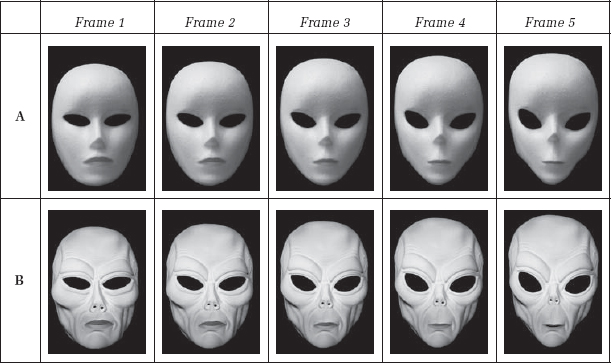
Figure 8-52: The A and B Sides of the Warp
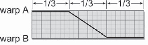
Figure 8-53: Typical Morph Cross-Dissolve Timing
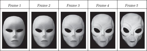
Figure 8-54: Dissolve Between A and B Side of the Warps to Make the Morph
8.3.3 Tips and Techniques
The single most important step in creating an excellent morph is to select appropriate images to morph between. What you are looking for in “appropriate images” is feature correlation—features in the two images that correlate with each other. The most mundane example is morphing between two faces—eyes to eyes, nose to nose, mouth to mouth, and so forth. The closer the two faces are in size, orientation of the head, and hairstyle, the better the morph will look. In other words, the more identical the A and B sides of the morph are, the easier it is to make a good morph.
If a face were to be morphed to a non-face target, say the front of a car, then the issue becomes trying to creatively match the features of the face to the “features” of the car—eyes to headlights and mouth to grill, for example. If the task is to morph a face to a seriously non-face target, say a baseball, the utter lack of features to correlate to will result in a morph that simply looks like a mangled dissolve. This is because without a similar matching feature on the B side of the morph to dissolve to, the black pupil of the eye, for example, just dissolves into a white leather region of the baseball. It is high-contrast features dissolving like this that spoil the magic of the morph.
Meanwhile, back in the real world, you will rarely have control over the selection of the A and B sides of the morph and must make do with what you are given. It is entirely possible for poorly correlated elements to result in a nice morph, but it will take a great deal more work, production time, and creative imagination than if the elements were well suited to begin with. Following are some suggestions that you may find helpful when executing morphs with poorly correlating elements:
- Having to warp an element severely can result in unpleasant moments of grotesque mutilation during the morph. Scale, rotate, and position one or both of the elements in order to start with the best possible alignment of features before applying the warps to minimize the amount of deformation required to morph between the two elements.
- Occasionally it may be possible to add or subtract features from one or the other of the elements to eliminate a seriously bad feature miscorrelation. For example, in the face-to-car example, a hood ornament might be added to the car to provide a “nose feature” for the car side of the morph. It probably wouldn't work to remove the nose from the face, however.
- When uncorrelated high-contrast features look “dissolvey,” such as a pupil dissolving into the white part of the baseball, try warping the offensive element to a tiny point. It will usually look better shrinking or growing rather than dissolving.
- Don't start and stop all of the warp action simultaneously. Morphs invariably have several separate regions warping around, so start some later than others to phase the action. A large deformation might start soonest so it will not have to change shape so quickly, calling attention to itself in the process.
- Don't do the dissolve between the entire A and B sides all at once. Separate the dissolve into different regions that dissolve at different rates and at different times. The action will be more interesting if it doesn't all happen at once. Perhaps a region on the B side looks too mangled, so hold the A side a bit longer in this region until the B side has had a chance to straighten itself out.
- The warps and dissolves need not be simply linear in their action. Try to ease in and ease out on the warps and the dissolves. Sometimes the warps or dissolves look better or more interesting if the speed is varied over the length of the shot.