
CHAPTER 5
The Composite
We have pulled our finest matte, refined it, and despilled the foreground layer. Now it is time to bring everything together in the composite. This chapter examines in detail the three steps within the compositing operation itself with an eye toward what goes on inside the typical compositing node. After a clear understanding of the compositing operation, some suggestions on how to refine and improve the overall appearance of all composites are offered.
When compositing cgi (computer-generated images), some special issues surface for color correction operations. The cgi comes to you “premultiplied,” which is an unnatural state for color correcting. Understanding what this is and how it affects the process is essential to understanding the fix—the “unpremultiply” operation— and its associated issues. We will also explore some alternative image blending techniques beyond the simple composite, namely the screen operation, the image multiply, and the much maligned maximum and minimum operations.
The matte has been around a long time and is used by several different professional disciplines. Of course, each group had to give it their own name. In deference to the different disciplines involved in compositing, the following conventions have been adopted. If we are talking about a matte used to composite two layers together such as with a bluescreen shot, it will be called a matte. If we are talking about the matte that is rendered with a four-channel cgi image for compositing, it will be called an alpha channel (or just the alpha). If we are talking about the matte used to composite two layers in a video context, it will be called a key. The names have been changed but the functions are the same. It still arbitrates the relative proportions of the foreground and background in the composited image.
5.1 The Compositing Operation
The compositing operation is the fundamental image combining operation of, well, digital compositing. The process is essentially the same, even when done optically—there is a foreground layer, a background layer, a matte to identify which region is which, and the final composited results. In addition to defining where the foreground and background appear in the frame, the matte also controls the degree of foreground transparency. The key elements of a basic composite are illustrated in Figure 5-1.
The compositing operation consists of three steps. The foreground is scaled (multiplied) by the matte, the background is scaled by the inverse of the matte, and then the results are summed together. Each of these operations will be explored in detail. The fact that these operations are performed digitally today offers an unprecedented level of control and quality.

Figure 5-1: The Elements of a Composite
5.1.1 Inside the Compositing Operation
In this section we peer inside a typical compositing node to understand its internal behavior. When you understand the math and operations that go on in the process you will be much better equipped to quickly troubleshoot problems and develop work-arounds. By the end of this section you will be able to make your own compositing node from simple discrete arithmetic nodes. Not that you will ever need to, of course, but it would be an interesting exercise of your command of the process.
A word to the folks who are working with log images. The compositing operation is one of the operations that must be done in linear space. You must convert both the foreground and background layers to linear (not the matte, since it is already a linear element), then convert the composited results back to log space.
5.1.1.1 Scaling the Foreground Layer
The foreground layer needs to be made transparent in the regions where the background is to be seen, and partially transparent in any semi-transparency regions, including the blending pixels that surround the foreground object (the woman, in the case of Figure 5-1). The pixels that are to become transparent are simply scaled to zero, and the semi-transparent pixels are partially scaled toward zero. This is achieved by multiplying each of the three channels of the foreground layer by the one channel matte. This assumes a “positive” matte—a white region where the foreground is to be opaque—and normalized pixel values, where white is 1.0 instead of 255. Multiplying the foreground layer by the matte channel scales each pixel in the foreground by the value of its matching matte pixel. Let's take a closer look at some pixels to see how they behave when scaled by the matte channel.
Figure 5-2 illustrates the three matte pixel cases, which is 100 percent opacity, partial transparency, and 100 percent transparency. The matte pixels are 1.0 for 100 percent opaque, 0.5 for 50 percent transparent, and 0 for 100 percent transparent. When a pixel in the RGB layer is scaled by the matte channel, all three channels are multiplied by the one matte pixel value.
The foreground in Figure 5-2 is represented by three identical pixels representing a skin tone with RGB values of 0.8 0.6 0.4. What starts out as three identical skin pixels will end up as three totally different scaled foreground values based on the values of the matte pixels. The resulting three foreground skin pixels are scaled to three different values: 0.8 0.6 0.4 for the 100 percent opaque skin (no change), 0.4 0.3 0.2 for the 50 percent transparent skin (all values scaled by 0.5), and 0 0 0 for the completely transparent skin (all zero pixels). It is the process of scaling the foreground pixel values toward black that makes them appear progressively more transparent.
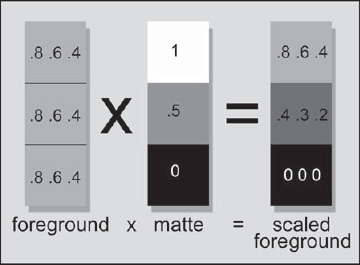
Figure 5-2: Multiplying the Foreground by the Matte

Figure 5-3: Multiplying the Foreground Layer by the Matte to Produce the Scaled Foreground Image
Figure 5-3 illustrates the matte multiply operation on the foreground layer to produce the scaled foreground image. Where the matte channel is zero black, the scaled foreground layer will also be zero black. Where the matte channel is 1.0, the foreground layer is unchanged. Any matte pixels that are between zero and 1.0 scale the foreground pixels proportionally.
5.1.1.2 Scaling the Background Layer
The foreground layer now has black where the background is going to be seen, so the background now needs to have black where the foreground is to be seen. You can think of it as punching a black hole in the background where the foreground object is to go. A similar scaling operation needs to be done on the background to suppress the pixels to black behind the foreground object. The difference is that the matte must be inverted before the multiply operation in order to reverse the regions of transparency.
Figure 5-4 illustrates how the background layer is multiplied by the inverted matte to produce the scaled background layer. The background layer now has a region of zero black pixels where the foreground is going to go.
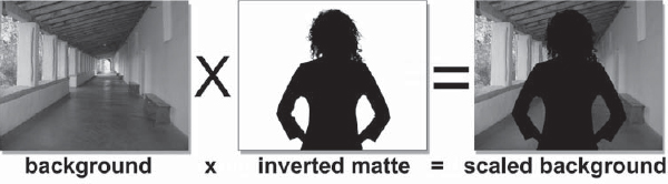
Figure 5-4: Multiplying the Background Layer by the Inverted Matte to Produce the Scaled Background Image
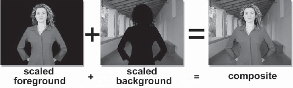
Figure 5-5: Summing the Scaled Background and Foreground to Create the Composite
5.1.1.3 Compositing the Foreground and Background
Once the foreground and background layers have been properly scaled by the matte channel, they are simply summed together to make the composite, as shown in Figure 5-5.
Figure 5-6 shows the flowgraph for building your own compositing operation from simple discrete nodes. The foreground layer (FG) is multiplied by the matte, again assuming a white matte, to make the scaled foreground. The background layer (BG) is multiplied by the inverted matte to make the scaled background. The scaled background and scaled foreground are then simply summed together in the add node.
The complete sequence of operations can also be seen by inspecting the official mathematical formula for a composite shown in Equation 5-1.
Composite = (matte FG) + ((1 – matte) × BG)(Eq. 5-1)
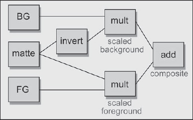
Figure 5-6: Flowgraph of Discrete Compositing Nodes
In plain English it reads “multiply the foreground by the matte, multiply the background by the inverted matte, then add the two results together.” Equation 5-1 could be entered into a channel math node and the composite performed that way.
5.1.2 Making a Semi-Transparent Composite
There is often a need for a semi-transparent composite, either to do a partial blend of the layers or to perform a fade up or fade down. To achieve a partial transparency, the matte simply needs to be partially scaled down from 100 percent white. The further away from 100 percent white the matte becomes, the more transparent the composite. Simply animating the matte scaling up or down will create a fade up or fade down.
Note that the foreground scaled matte in Figure 5-7 appears as 50 percent gray in the white region. You can see how this partial density is reflected in the partially scaled foreground and background, which in turn shows up in the final composite as a semi-transparency.
Figure 5-8 shows how the flowgraph would be modified to introduce semi-transparency or a fade operation. The scale node is added to bring the white level down on the matte, which controls the degree of transparency. The scaled matte is then used to scale both the foreground and background in the multiply nodes.
Equation 5-2 has a transparency scale factor added which is represented by the letter z. When z is zero, the foreground is completely transparent. When it is 1.0, the foreground is completely opaque, and a number between zero and one will produce a partial transparency.
((z × matte) × FG) + ((1 – (z × matte)) × BG)(Eq. 5-2)
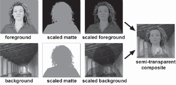
Figure 5-7: A Semi-Transparent Composite
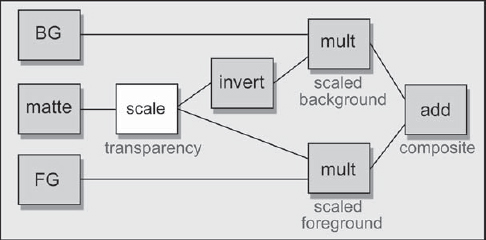
Figure 5-8: Flowgraph of Semi-Transparent Composite
5.2 The Processed Foreground Method
We saw in the previous section the classical method of compositing—multiply the foreground layer by the matte, multiply the background layer by the inverse of the matte, then sum the two together. But there is another way, a completely different way, which might give better results under some circumstances. It is called the processed foreground method because it is modeled after Ultimatte's method of the same name. Its main virtue is that it produces much nicer edges under most circumstances than the classic compositing method.
5.2.1 Creating the Processed Foreground
The processed foreground method is essentially a different way of scaling the foreground by the matte to clear the surrounding backing color pixels to zero. With the classical compositing equation this is done by multiplying the foreground layer by its matte to produce the scaled foreground. With the processed foreground method a separate plate called the backing plate is created, which is the same color as the backing color. The matte is used to clear to black the area where the foreground object is located, and then it is subtracted from the original foreground layer, which clears the backing region to black. Here is how it works.
Referring to Figure 5-9, the first step is to create a backing plate, which is nothing more than a plate of solid color with the same RGB value as the green (or blue) backing color of the foreground layer. The backing plate is then multiplied by the inverted matte to create the scaled backing plate. The scaled backing plate represents a frame of the backing color with zero black where the foreground element used to be. When this is subtracted from the original foreground layer, the backing region of the foreground layer collapses to zero black, leaving the foreground object untouched. The processed foreground now appears to be identical to the scaled foreground created in Figure 5-3. But appearances can be deceiving.
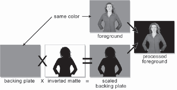
Figure 5-9: Creating the Processed Foreground
If you were to use the same matte to make a scaled foreground and a processed foreground, and then compared the two, you would find that the processed foreground version has a kinder, gentler edge treatment. The edge pixels in the scaled foreground version will be darker and show less detail than the processed foreground version. The reason for this can be understood by taking an example of an edge pixel with a matte value of 0.5. With the scaled foreground, the RGB value of the edge pixel will be multiplied by 0.5, reducing the pixel value by half. With the processed foreground method the same 0.5 matte value will be used to scale the backing plate color in half, then this RGB value is subtracted from the original foreground RGB value. In all cases this will reduce the foreground RGB value by less than the scaling operation, which results in a brighter pixel value for the processed foreground method. Hence, less dark edges.
Figure 5-10 shows the flowgraph for creating a processed foreground. Starting with the foreground (FG), a matte is pulled using your best method, then it is inverted. A backing plate is created simply by filling a solid color node with the RGB value of the backing color. The backing plate is then multiplied by the inverted matte and the results are subtracted from the foreground.
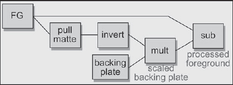
Figure 5-10: Flowgraph for Creating a Processed Foreground
5.2.2 Compositing the Processed Foreground
When using the processed foreground method, the compositing operation itself must be modified. With the classical compositing method the comp node is given the original foreground layer, which is scaled within the comp node to create the scaled foreground. With the processed foreground method the foreground layer is already “scaled” and we do not want to scale it again in the comp node. This means that the foreground scaling operation must be turned off in the comp node.
Another issue is where to put the despill operation. The processed foreground will have much of the edge contamination removed, but there are still spill and veiling to deal with. The despill operation is placed after the processed foreground and before the comp node, as shown in Figure 5-11. Again, be sure to turn off the foreground multiply operation in the comp node to avoid double-scaling the foreground layer and introducing some very nasty dark edges.
5.2.3 Some Issues
Although the processed foreground method has the advantage of softer edges, it also has its problems and limitations. One of its problems is that it will introduce some residual grain over the background plate that is “inherited” from the backing region of the foreground layer. Another limitation is that it is less tolerant of unevenly lit greenscreens. The classical scaled foreground method is immune to these problems because the entire backing region is scaled to zero based on the value of the matte regardless of the pixel values of the backing region in the foreground layer. With the processed foreground method the pixel values of the backing region do affect the results.
5.2.3.1 Residual Grain
Figure 5-12 shows why residual grain from the backing region will end up on the background plate after the composite. The jaggy line labeled “A” represents the typical grain pattern of the backing region of a foreground plate. The flat line labeled “B” represents the backing plate that was created for it. The average RGB value of the foreground plate was sampled in the backing region, then these values were used to fill a constant color node with a matching color. However, the synthesized backing plate has no grain, hence the perfectly flat line “B.” Any grain pixels in the foreground layer (A) that are greater than the backing plate (B) will be left over after the scaled backing plate is subtracted from the foreground. These residual grain pixels are represented by line “C” in Figure 5-12.
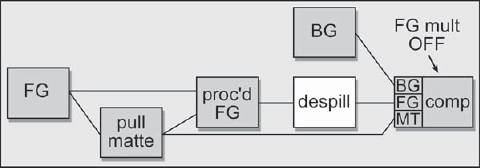
Figure 5-11: Flowgraph of Processed Foreground Compositing

The residual grain pixels will be lurking in what appears to be the zero black region of the processed foreground and may become quite visible after the composite. They will end up “on top” of the background plate everywhere the backing region used to be in the foreground layer. Ultimatte also exhibits this behavior, and for the same reason. A reasonable amount of this residual grain is not a problem. If the residual grain becomes a problem, the RGB values of the backing plate can be tapped up a bit so that they will subtract more from the foreground plate, leaving less residual grain. Since the blue channel has the most grain, it will be the one needing the most tapping. Be sure to raise the RGB values by the least amount necessary to lower the residual grain to an acceptable level. The more you raise the backing plate RGB values, the more it degrades the edges.
5.2.3.2 Uneven Backing Colors
Another problem that can occur with the processed foreground method is backing region residuals due to uneven greenscreens. An example would be where the backing region is unevenly lit or made up of several panels that are not all the same color. The slice graph in Figure 5-13 illustrates a situation where there is a lighter panel on the left. The slice line “A” shows the two levels of brightness of the backing region, and “B” again shows the single RGB value of the backing plate. When the scaled backing plate is subtracted from the foreground plate the lighter region will leave a major residual shown by the slice line at “C.” This residual will also end up being added to the background layer of the final composite. This is also a trait of the Ultimatte process.
There are a couple of fixes for this. One fix is to garbage matte the backing region. This sets that backing region to a constant RGB color that can perfectly match the backing plate color. Of course, the region close to the foreground object that is not garbage matted will still show a bit of the grain. The other fix is to use screen correction, which was covered in Chapter 2, “Pulling Mattes.”

Figure 5-13: Uneven Backing Residual
5.3 Refining the Composite
In this section we will explore some processes that can be done during and after the composite operation to refine the quality further. Even after the best matte extraction and matte refinement efforts, the final composite will often have less than beautiful edge transitions between the composited foreground and the background. Performing a little edge blending after the final composite will better integrate the composited layers and “sweeten” the look of the finished work. The soft comp/hard comp technique is a double compositing strategy that dramatically improves edge quality and density for troublesome mattes. It takes advantage of two different mattes—one that has best edges and one that has best density—retaining the best of both worlds without introducing any artifacts itself.
5.3.1 Edge Blending
In film compositing a “sharp” edge may be three to five pixels wide, and soft edges due to depth of field or motion blur can be considerably wider. A convincing composite must match its edge softness characteristics to the rest of the picture. Very often the matte that is pulled has edges that are much harder than desired. Blurring the edges of the matte is very often done, but has the down side of blurring out fine detail in the matte edge. A different approach that gives a different look is edge blending—blending the edges of the foreground object into the background plate after the final composite. It can result in a very natural edge to the composited object, which helps it to blend into the scene. Of course, an artistic judgment must be made as to how soft the edge should be to blend well into the scene, but you will find that virtually all of your composites will benefit from this refinement, especially feature film work.
The procedure is to use an edge detection operation on the original compositing matte to create a new matte of just the matte edges, like the example in Figure 5-14. The width of the edge matte will vary, of course, but will typically be three or four pixels wide for film resolution work, and obviously much thinner for video work. Again, the width of the edge matte is a case-by-case artistic judgment.

Figure 5-14: Edge Blending Matte Created from Original Compositing Matte
The edge matte itself needs to have soft edges so that the blur operation does not end with an abrupt edge. If your edge detection operation does not have a softness parameter, then run a gentle blur over the edge matte before using it. Another key point is that the edge matte must straddle the composited edge of the foreground object, like the example in Figure 5-16. This is necessary so that the edge blending blur operation will mix pixels from both the foreground and background together, rather than just blurring the outer edge of the foreground.
Figure 5-15 is a close-up of the original composite with a hard matte edge line. Figure 5-17 shows the resulting blended edge after the blur operation. Be sure to go light on the blur operation and keep the blur radius small—one or two pixels—to avoid smearing the edge into a foggy outline around the entire foreground.
Figure 5-18 is a flowgraph of the sequence of operations for the edge blending operation on a typical greenscreen composite. An edge detection is used on the compositing matte to create the edge matte. The edge matte is then used to mask a gentle blur operation after the composite.
Figure 5-15: Original Composited Image

Figure 5-16: Edge Matte Straddles Composite Edge

Figure 5-17: Resulting Blended Edge

Figure 5-18: Flowgraph of Edge Blending Operation
5.3.2 Soft Comp/Hard Comp
This is one of the most elegant solutions to the chronic problem of poor matte quality. It seems that there are always two conflicting matte requirements. On the one hand you want lots of fine detail in the edges, but you also want 100 percent density in the foreground area. In most cases these are mutually exclusive requirements. You can pull a matte that has lots of great detail around the edges, but the matte has insufficient density to be completely opaque. When you harden up the matte to get the density you need, the edge detail disappears and you get the “jaggies” around the edge. The soft comp/hard comp procedure provides an excellent solution for this problem and, best of all, it is one of the few procedures that does not introduce any new artifacts that you have to go pound down. It's really clean. This technique can also be used very effectively with keyers such as Ultimatte.
The basic idea is to pull two different mattes and do two composites. The first matte is the “soft” matte that has all of the edge detail, but lacks the density to make a solid composite. This soft matte is used first to composite the foreground over the background, even though the foreground element will be partially transparent. The matte is then hardened by scaling up the whites and shrinking it a bit. This produces a hard-edged matte that is slightly smaller than the soft matte and fits “inside” of it. This hard matte is then used to composite the same foreground layer a second time, but this time the previous soft composite is used as the background layer. The hard comp fills in the semi-transparent core of the soft comp, with the soft comp providing fine edge detail to the overall composite. The best of both worlds. Figure 5-19 illustrates the entire soft comp/hard comp process.
Here are the steps for executing the soft comp/hard comp procedure:
Step 1: Create the “soft” matte. It has great edge detail, but does not have full density in the core.
Step 2: Do the soft comp. Composite the foreground over the background with the soft matte. The partially transparent composite is expected at this stage.
Step 3: Create the hard matte. It can be made either by hardening and shrinking the soft matte, or by pulling a new matte using more severe matte extraction settings to get a harder matte. Either way, the hard matte must be 100 percent solid and a bit smaller than the soft matte so that it does not cover the soft comp's edges.
Step 4: Do the hard comp. Comp the same foreground again, but use the soft comp as the background. The hard matte fills in the solid core of the foreground, and the soft comp handles the edge detail.

Figure 5-19: Soft Comp/Hard Comp Sequence of Operations
In a particularly difficult situation you could consider a three-layer composite, with each layer getting progressively “harder.” Any edge blending would be done only on the outermost layer, of course.
5.3.3 Layer Integration
The two previous sections were concerned with refining the composite from an essentially technical point of view. Here we will look at refining a composite from an artistic point of view. In later chapters we will explore the role of matching color, lighting, and other aspects of the disparate layers to blend them together better by making them appear to be in the same lightspace. But while we are still looking at the compositing operation this is a propitious moment to point out that there is a compositing step that can be done to help “sell” the composite, and that is to integrate, or sandwich, the foreground layer within the background layer, rather than just lay it on top.
Figure 5-20 illustrates simply pasting the foreground layer over the background. In this example the castle is a foreground layer that has been created in Adobe Photoshop and then composited over the “live action” hill. While the composite looks very nice, the composite itself can be made even more convincing by integrating the castle into the background layer by sandwiching it between elements of the background.

Figure 5-20: Foreground over Background Without Integration (Courtesy of Glen Gustafson)

Figure 5-21: Foreground Integrated into the Background (Courtesy of Glen Gustafson)
In this particular example, some of the bushes of the background plate have been isolated, then laid back over the castle at its base in Figure 5-21. In addition to that, a foreground tree element has been added to further the sense of depth and integration of the castle into the scene. Of course, none of this is a substitute for properly color correcting the layers to match, but by layering the foreground element into the background with elements from the background plate itself, it will appear more to the eye to be a single integrated composition. It's a perception thing.
5.4 Compositing CGI Images
The explosion in the use of cgi in the movies and on television has brought with it an explosion in compositing cgi, and this trend will only increase in the future. On the surface, compositing cgi would seem a simple issue because it comes complete with its own perfect matte, the alpha channel. If all you have to do is slap the cgi over a background plate, life is indeed easy.
However, if you have to color correct the cgi, bad things begin to happen because the cgi is premultiplied—meaning that by the time you get it, it has already been multiplied by its alpha channel. This is the same operation that we use in regular compositing to scale the foreground by the matte. We have just referred to it as the scaled foreground rather than being premultiplied. The fundamental problem here is that the color correction operations should be done before the foreground is premultiplied (scaled by the matte), not after. We therefore need to perform an unpremultiply operation to the cgi prior to color correction to restore it to a color correctable state. Then we will see how to solve the problems that the unpremultiply operation can introduce. Suddenly, working with cgi is not so simple.
5.4.1 The Premultiplied CGI Image
When we were exploring the compositing operation in Section 5.1.1.1, “Scaling the Foreground Layer,” we saw in Figure 5-3 how the foreground layer is multiplied by the matte to produce the scaled foreground layer. The hallmark of a multiplied foreground image is that the foreground object is surrounded by black because the “not-foreground” pixels have all been scaled to zero. A cgi image is referred to as a premultiplied image because the RGB layer has already been multiplied by its matte (alpha). For regular image layers this operation is not done until the actual composite operation.
As a result of this premultiply operation the cgi object is already surrounded by zero black pixels and its edges are scaled toward black, so it is very important that the multiply operation not be applied a second time during the composite. If it is, the cgi object will be surrounded by a very unpleasant dark edge. Your problem is to determine how your composite node behaves so that you can turn off the foreground multiply operation when compositing cgi, but turn it on when compositing two regular image layers.
Figure 5-22 compares the behavior of premultiplied cgi images to regular image layers when composited incorrectly with the foreground multiply operation. The comparison is between two hypothetically identical balls, one a live action ball (a) shot on a greenscreen and the other a cgi ball (e). A white slice line has been draw across both balls and graphed next to each for comparison. The ball matte (i) has also been slice graphed so that you can see the shape of the matte used for the multiply operation. For purposes of this exercise, we will stipulate that the ball matte pulled from the greenscreen is identical with the alpha channel of the cgi ball. The live action slice (b) and the cgi slice (f) graphs look very different. The edges of the live action slice (b) rise to the value of the greenscreen, while the cgi slice (f) edges show the edges of the cgi ball dropping to zero black. Now comes the interesting bit.

Figure 5-22: Comparison of Compositing Results for Premultiplied CGI versus Unpremultiplied Live Action Foregrounds
In the top row of Figure 5-22 the multiplied live (c) slice graph shows how the edges of the live action ball have dropped to zero due to being multiplied by the matte. It now looks exactly like the premultiplied cgi in the cgi slice (f) graph. However, if the premultiplied cgi ball were also mistakenly multiplied by the matte, the consequences would be dire. The multiplied cgi (g) slice graph shows how the cgi ball edges have been dropped to zero black much harder after being scaled by the matte (arrows). The previous, proper edges are also shown as a dotted line for comparison. Note that the only pixels affected are those that have partial transparency alpha pixels with values other than exactly zero or one.
This unwarranted multiplying by the matte seriously darkens the pixels all around the foreground object's perimeter because these are partially transparent anti-aliasing pixels. When the composite is then performed, the cgi comp (h) will now exhibit this dark edge due to having the edge pixels double-scaled by the alpha channel—once during the cgi render, and again during the composite. The live action comp (d) above it has a proper edge for comparison. The solution is to turn off the foreground multiply operation (sometimes called the foreground scale) in the comp node when compositing a premultiplied cgi element.
5.4.2 The Unpremultiply Operation
The premultiplied form of cgi images introduces a special problem when it comes to color correcting. The interaction between the color correction and the compositing operation does not work properly in many cases, so color correcting the pre-multiplied image can result in color anomalies. The problem lies with those pixels in the RGB channels that sit over alpha channel pixels that are not a value of exactly 1.0—that is, all alpha pixels that are either partially transparent (anti-aliased edges and semi-transparent regions) or zero (background regions). The partially transparent and absolute zero alpha pixels each introduce a different problem. The zero value alpha pixels have the simplest problem, so we will start with them.
5.4.2.1 The Zero Black Alpha Pixel Problem
When the alpha channel of a cgi element has a zero black pixel it normally means that this part of the final composited image is supposed to be the background, so the RGB pixel values in this region are also supposed to be zero black. Some color correction operations can raise these black RGB pixels above zero, giving them some color where they should be zero black. Under normal circumstances this would be no problem because these “colorized” black pixels would be scaled back to zero black during the compositing operation.
However, as we saw in Section 5.4.1, “The Premultiplied CGI Image,” with pre-multiplied cgi images the foreground multiply operation must be turned off. This means that any colorized black pixels in the cgi layer are no longer scaled back to black, so they end up being summed with the background layer, discoloring it. Since we cannot turn the foreground multiply operation on to clear them out lest we double-multiply the cgi by the alpha channel (a very bad thing to do), something must be done to prevent them from appearing in the first place. In principle, you could use the alpha channel itself to mask off the color correction from the black pixels, but that still leaves the second problem—the partially transparent alpha pixels.
5.4.2.2 The Partially Transparent Alpha Pixel Problem
This is a somewhat messier problem than the zero black pixels and requires a bit of math to sort out because the problem is introduced by the interaction of the foreground scale operation and the color correction operation. This little drama has three players: the RGB value of the “true” color of the cgi object, the alpha pixel transparency, and the color correction operation. By “true” color I mean the RGB value the cgi object has before it is scaled by the alpha channel during the render premultiply operation. The sequence of operations for a typical bluescreen (unpre-multiplied) composite is:
- “True” RGB value (original color)
- Color correction (done by the artist)
- Scale foreground by matte (performed in the comp node)
A cgi element has already been scaled by the alpha channel before you get it to composite. In this case the order of operations has become:
- “True” RGB value (original color)
- Scale foreground by alpha (performed during the render)
- Color correction (done by the artist)
Swapping the order of the color correction and scale foreground operations is harmless if they are both multiply operations for the same reason that 2 × 3 × 4 is equal to 3 × 4 × 2. In other words:
“true” RGB × color correction alpha = “true” RGB × alpha color correction
The scale foreground operation is always a multiply operation, but the color correction is not. There are some color correction operations that might perform an add operation or a scale with an offset. In this case, the order of operations suddenly becomes critical for the same reason that (2 + 3) × 4 is not equal to (3 × 4) + 2. The order of operations produces very different results when it is not restricted to multiply operations only.
How this all relates to your personal composite can best be understood by taking a specific example and comparing the results. Let's assume that we are rendering a cgi object and our test pixel has an RGB value of 0.6 (to simplify the problem, all three channels have the same data). Let's also say that our test pixel is partially transparent. Why it is transparent is not important—it could be either that it is within a semi-transparent surface or that it is an anti-aliased edge pixel of a solid surface. Either way, let's say that its alpha pixel value is 0.5, meaning it is 50 percent opaque (or 50 percent transparent, if you prefer).
When our test pixel is rendered out to a file and given to you to composite, it will not have its “true color” value of 0.6. It will have been premultiplied by its alpha pixel value (0.5), so the pixel you will see on the screen will be 0.3 (0.6 × 0.5). The pixel value of 0.6 only existed within the render before the image was multiplied by the alpha channel and output to a file, but that is the true color of the surface in question. Let us assume for the color correction that we simply wish to add a value of 0.2 to our test pixel and compare the results of using a premultiplied versus an unpremultiplied pixel. Although plowing through the following math operations may be a bit tedious, it demonstrates the problem with color correcting unpremultiplied images.
Starting with the left-hand column of Table 5-1, which has the correct unpre-multiplied sequence of operations, the true RGB value of 0.6 gets the 0.2 color correction added to it for a color corrected pixel value of 0.8. After the color correction, it is multiplied by the alpha pixel value of 0.5 to result in the correct pixel value of 0.4. The key is that the color correction was done to the true pixel value (0.6) before it was multiplied by the alpha channel. It is the color corrected true pixel value that should get multiplied by the alpha.
Referring to the right-hand premultiplied column in Table 5-1, let's follow the action and track what happens to the test pixel when a premultiplied pixel is color corrected before being composited. The true RGB value of the test pixel starts out as 0.6, gets multiplied by the alpha pixel value of 0.5, and results in a pixel value of 0.3 to you at your workstation. A value of 0.2 is then added to it in the color correction operation for a resulting pixel value of 0.5. Color this the wrong result. Somehow we must undo the premultiply operation to restore the true color, apply the color correction, then re-multiply it by the alpha channel.
Undoing the premultiply is called an unpremultiply, and it turns out that this is easy to do. The method is to simply divide the cgi image by its own alpha channel. This “backs out” the premultiply operation done at rendering time, restores the partial transparency pixels back to their original RGB values, and permits totally correct color operations to occur. Let's take a closer look at three unpremultiply cases. The setup for the three cases is that the RGB value is 0.6, and there are three alpha pixel values to examine: one at 1.0 (full opacity), one at 0.5 (partial transparency), and one at zero (full transparency), shown in Table 5-2. To unpremultiply a pixel, we simply divide it by its alpha pixel.
Case 1 in Table 5-2 is where a pixel with a true color of 0.6 is over a completely opaque alpha pixel. To make the premultiplied value, the true color is multiplied by the alpha value of 1.0, resulting in an output pixel to you of 0.6. The premultiply operation did not modify the true color of the pixel, and since the unpremultiply operation divides by 1.0, the true color is left untouched.
Case 2 is where a pixel with a true color of 0.6 is over a partially transparent alpha pixel. To make the premultiplied pixel value, the true color is multiplied by the alpha value of 0.5, resulting in an output pixel of 0.3. When it is unpremulti-plied, the premultiplied value of 0.3 is divided by the alpha of 0.5, resulting in an unpremultiplied value of 0.6. We have magically restored the true color of the pixel. However, in so doing any anti-aliased pixels will no longer fade to black at the edges. The unpremultiplied image takes on very jaggy edges. Not to worry; this will be fixed during the composite.
Case 3 is the case where the zero black surround pixels are over zero black alpha pixels. These are the totally transparent pixels surrounding the rendered cgi object. When these are unpremultiplied, zero is divided by zero, which is infinity. Most compositing packages do not handle pixel values of infinity, so the output of the divide node will be clipped to 1.0 (white). This means that the cgi object is suddenly surrounded by white pixels, which will look bizarre, but is nothing more than a visual annoyance. The white will be cleared out later, during the composite. I just wanted to give you a heads up on this little issue so you wouldn't freak when you first saw it.
Some software packages have an unpremultiply node that fixes the annoying white surround problem by simply dropping to black all pixels that are over zero black alpha pixels. It is comforting to see the cgi object still surrounded by black, but of course the anti-aliased pixels will still have a serious case of the jaggies when they are unpremultiplied.
REALITY CHECK
In the real world, if the color correction to be applied to the cgi is small, the error it introduces is small, so you might be able to ignore the whole unpremultiply thing.
There are two reasons for dragging you through the unpremultiply mud. The first is so that you will understand when and why this operation is needed, and how to adjust the compositing operation for it (the very next section). The second reason is to set you up for understanding the hideous artifact that the unpremultiply operation can introduce.
5.4.3 Adjusting the Composite for Unpremultiplied CGI
In Section 5.4.1, “The Premultiplied CGI Image,” we saw that the foreground multiply operation must be turned off to avoid double-scaling the foreground layer when compositing a premultiplied image. But now that we have an unpremultiplied image, the foreground multiply operation must be turned back on. Figure 5-23 illustrates a flowgraph of the operations for the unpremultiplied cgi composite. The premultiplied cgi goes to an unpremultiply node (or a divide node if you don't have unpremultiply), and the unpremultiplied cgi is color corrected. The color corrected unpremultiplied cgi goes to the comp node, where the foreground multiply operation is enabled. With the foreground multiply operation enabled, even if the color correction operation contaminates the “black” transparent pixels in the cgi image, they will all be cleared back to black during the composite.
Here is a summary of the rules of thumb:
- If you do not have to color correct the cgi image, leave it premultiplied, and composite with the foreground multiply operation OFF.
- If you must color correct the cgi image, umpremultiply it, perform the color correction, and composite with the foreground multiply operation ON.
It is very important to be clear on this, because mismatching your cgi unpremultiply state with your compositing foreground multiply enable is guaranteed to give you raunchy comps. It even sounds painful.
5.4.4 Unpremultiply Highlight Clipping
Here is the hideous artifact I promised you. There are certain situations where the unpremultiply operation can clip the pixel RGB values. This occurs when any of the three RGB values of a pixel is greater than its alpha pixel value. Take, for example, a pixel with an RGB value of 0.5 0.7 0.8 and an alpha pixel value of 0.6. In this example the G pixel (0.7) and the B pixel (0.8) are greater than the alpha pixel (0.6) and will be clipped during the unpremultiply operation. Diabolically, the clipping will not be visible until the cgi element is composited.
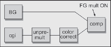
Figure 5-23: Flowgraph of Unpremultiply Composite
This condition can occur when a reflective highlight is rendered on a semi-transparent surface, such as a specular kick on a glass object. The example in Figure 5-24 represents a semi-transparent glass ball with a specular highlight reflecting off the top. The original rendered highlight is shown in (a) and the clipped highlight after the composite in (b). The clipping has introduced an ugly “flat” spot in the center of the highlight.
5.4.4.1 What Goes Wrong
Virtually all software packages clip any normalized pixel values that exceed 1.0. Under certain conditions, the unpremultiply operation can result in pixel values greater than 1.0, so they get clipped. When these clipped pixels get composited, they produce the clipped “flat” spot in the highlights. Here is how it happens.
For a typical solid or even semi-transparent surface, the cgi render outputs a pre-multiplied RGB pixel value that is less than its associated alpha pixel value: for example, an RGB value of 0.4 and an alpha value of 0.8. The unpremultiply operation performed at compositing time divides the RGB by the alpha, so it is dividing a smaller number by a larger number, which is always less than one (0.4 ÷ 0.8 = 0.5). With the results less than one there is no clipping.
However, for a semi-transparent surface with a lens flare or a specular highlight (a glint), the RGB value will often exceed the alpha value. A larger RGB number is then being divided by a smaller alpha number. This results in an unpremultiplied value greater than one, which is promptly clipped by the compositing software to 1.0. The clipped values have been “shaved off” the top of the pixels; then after the composite operation the missing color data appears as the clipped regions. In fact, whenever any color channel of a premultiplied cgi pixel exceeds its alpha value, it will be clipped to its alpha channel value, producing flat spots in the highlights. If this happens to one or two channels it will also result in color shifts in the clipped areas.
MATH EXEMPTION
For those sturdy folks who are interested in the details of the math involved in the unpremultiply highlight clipping artifact, the following section is offered. If you are not interested in the math you may skip this section and go straight to Section 5.4.4.2, “How to Fix It,” with negligible harm to your career.

Figure 5-24: CGI Highlights: (a) rendered highlight, (b) clipped highlight
Understanding the details of the unpremultiply highlight clipping is mathematically tedious because the pixel values must be tracked through a series of rendering and compositing operations. Three cases are illustrated in Table 5-3. Each case is first tracked through the cgi render operations, then into the compositing operations. To avoid clipping, the scaled FG value in the composite must be the same as the output value from the render. Again, for the sake of simplicity, all channels have the same value.
Case 1 is a completely opaque pixel, so its alpha value will be 1.0. During the render, the premultiply operation is performed by multiplying the true RGB value by the alpha, so the premultiplied pixel value is 0.9 × 1.0 = 0.9. There is no highlight, so the final render output value is also 0.9. Following it into the compositing operations, when we perform the unpremultiply, the RGB is divided by the alpha to get the true RGB value back, which is 0.9 ÷ 1.0 = 0.9. Because the RGB is less than the alpha the unpremultiplied results did not exceed 1.0, so this pixel is not clipped. When it is multiplied by its alpha to calculate the scaled FG, its value is 0.9 × 1.0 = 0.9, identical with its original output value, which is what we want.
Case 2 is the same pixel as above, but this time it is semi-transparent. Its true RGB value is still 0.9, but now its alpha value is 0.5. Its premultiplied value will now be 0.9 × 0.5 = 0.45, and again there is no highlight, so the rendered output is still 0.45, which is what you would see on your monitor. The RGB output value (0.45) is still less than the alpha value (0.5). When it gets into the compositing operation the unpremultiply operation is applied, with the results of 0.45 ÷ 0.5 = 0.9, magically restoring the true RGB value. This is again less than one, so there is no clipping. When scaled by the alpha channel during the composite, the scaled FG value is 0.9 × 0.5 = 0.45, again identical with the original output value.
Case 3 is the same semi-transparent pixel, but this time we will add a specular highlight to it. Its true RGB value is still 0.9 from the original surface and the alpha value is still 0.5, so the premultiplied version is still 0.9 × 0.5 = 0.45. But now the cgi render adds the specular highlight after the premultiply operation because it “lies on top” of the surface, so is unaffected by its transparency. Let's say its value is 0.25, so the final output pixel you get is 0.45 + 0.25 = 0.7. This is greater than the alpha value of 0.5. Now, in compositing, we perform the unpremultiply operation and we get 0.7 ÷ 0.5 = 1.4, which is greater than one, so it gets clipped back to 1.0. This time, when it is scaled during the composite, the scaled FG value becomes 1.0 ÷ 0.5 = 0.5, which is way off from the original rendered value of 0.7. This becomes the clipped region of the highlight in the final composite.
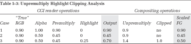

Figure 5-25: Flowgraph of Pre-Scaled Unpremultiply Operation
5.4.4.2 How to Fix It
There are two general approaches to fixing the unpremultiply highlight clipping artifact. The first solution, which I strenuously recommend, is to render the highlights as a separate layer and composite them separately. It's simple, easy, and works every time. It also allows separate control of the highlight at composite time, and operations other than compositing can be used to mix it in. The second solution is to pre-scale the cgi. This is a bit more obtuse and entails the use of some math.
As explained earlier, the fundamental problem with the highlight pixels is that their RGB values exceed their alpha values. This results in unpremultiplied values that exceed a value of one, which in turn get clipped. This problem can be solved by pre-scaling the RGB values of the cgi layer down until the greatest RGB value is at or below its alpha value prior to the unpremultiply operation. With all RGB values less than their alpha values the unpremultiply operation will no longer produce any values that exceed one, so there is no clipping. The background plate must also be scaled by exactly the same amount, then the finished composite unscaled to restore its original brightness. Of course, the alpha channel itself is not scaled. The flowgraph for the pre-scaled unpremultiply operation is shown in Figure 5-25.
Let's say that you had to scale the RGB channels down by 0.5, then performed the unpremultiply operation followed by the color correction. The background plate must also be scaled down by 0.5 before the two layers are composited. Since the foreground is now unpremultiplied, the scale foreground operation is on. The resulting composite is then scaled back up by the inverse of the original scale factor to restore all brightness levels. In this example it is 1 ÷ 0.5 = 2.0. Of course, these scaling gyrations cannot be done on 8-bit images without introducing serious banding. The cgi renders and background plates must both be 16-bit images. The color correction operation (which is why you are bothering with the unpremultiply in the first place) is done after the unpremultiply and before the composite, as usual.
5.5 Other Ways to Blend Images
Compositing is not the only way to blend two images together. It is very appropriate for placing solid object A over solid background B, but there are whole categories of other visual, atmospheric, and light phenomena that look much better with other methods of image blending. In this section we will explore matte-less compositing techniques using the screen operation, a mighty useful alternative way of mixing light elements such as flashlight beams and lens flares with a background plate. We will also examine the multiply operation, which, when properly set up, can provide yet another intriguing visual option for the modern digital compositor. For those occasions where suitable elements are available, the maximum and minimum operations can also be used to surprising advantage.
5.5.1 The Screen Operation
The screen operation is a very elegant alternative method to combine images. It is not a composite. It does not use a matte, and it gives very different results from a composite. Perhaps the best way to describe its purpose is when you want to combine the light from one image with a background picture, as in a double exposure. One example would be a lens flare. Other examples would be the beam for an energy weapon (ray gun), or adding a glow around a light bulb, fire, or explosion. The key indication that it is time to use the screen operation is when the element is light-emitting and does not itself block light from the background layer. Fog would not be a screen candidate because it obscures the background, blocking its light from reaching the camera. Composite your fogs. (Thin wisps of dust or smoke can sometimes be screened in.)
Figure 5-26 shows an example of a lens flare element for screening. One key point about the screen layer is that it is always over a zero black background. If any of the pixels are not zero black they will end up contaminating the background plate in the finished picture. Figure 5-27 shows the background plate, and Figure 5-28 shows the results of screening the lens flare over the background plate. Notice that the light rays are mixed with but do not actually block the background image. The dark pixels in the background plate behind the hot center of the lens flare may appear blocked, but they are just overexposed like a double exposure of a bright element with a dark element. The bright element dominates.
Figure 5-29 illustrates the “double exposure” behavior of the screen operation. It depicts two identical gradients, images A and B, screened together. The key characteristic to note here is how the maximum brightness approaches, but does not exceed, 1.0. As the two images get brighter, the screened results also get brighter, but at a progressively lesser rate. They become “saturated” as they approach 1.0, but cannot exceed it. When black is screened over any image the image is unchanged, which is why the screen object must be over a zero black background.

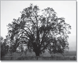
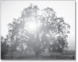
Figure 5-28: Lens Flare Screened over Background Plate

Figure 5-29: Results of Two Gradients Screened Together
5.5.1.2 Adjusting the Appearance
You cannot “adjust” the screen operation to alter the appearance of the results. It is a hard-wired equation somewhat like multiplying two images together. If you want the screened element to appear brighter, dimmer, or a different color, then simply color grade it appropriately before the screen operation. Again, be careful that none of your color grading operations disturbs the zero black pixels that surround the light element, because any black pixel values raised above zero will end up in the output image.
Some compositing programs actually have a screen node, and Adobe Photoshop has a screen operation. For those of you not blessed with a screen node, we will see how to use either your channel math node or discrete nodes to create a perfect screen operation. But first, the math. Following is the screen equation:
1– ((1 – image A) × (1 – image B))(Eq. 5-3)
In plain English it says “multiply the complement of image A by the complement of image B, then take the complement of the results.” In mathematics the complement of a number is simply 1 minus the number. The number, in this case, is each pixel of the image. Again, note that there is no matte channel in a screen operation. It just combines the two images based on the equation. This equation can be entered into a channel math node to create your own screen node.
In the event that you do not own a math node or don't want to use the one you do have, Figure 5-30 shows the flowgraph for “rolling your own” screen operation using simple discrete nodes in your compositing software. The screen element is first color corrected, if needed, then both images are “inverted” (some software may call this operation “negate”; in mathematics it is the “complement” operation used in Equation 5-3). They are then multiplied together and the results inverted. That's all there is to it. You can build this into a macro and save it out as your own personal screen node. You could even share it with your colleagues. Or not.
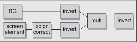
Figure 5-30: Flowgraph of Discrete Nodes for Creating a Screen Operation
5.5.2 The Weighted Screen Operation
A composite blocks the background layer, but the screen operation doesn't. There are times, however, when you would like to have the “glow” of the screen operation, but still suppress the background layer a bit. This is the time to use the weighted screen operation. The idea is to create a matte for the screen object (the light emitter) and use it to partially suppress the background layer prior to the screen operation. The matte can be generated any number of ways. Most commonly it is a luminance version of the screen object itself, or perhaps the alpha channel in the case of a cgi element. However it is done, a matte is needed for the weighted screen.
We can compare the results of a regular screen operation with the weighted screen operation starting with Figure 5-31, the screen element. Comparing the two background plates in Figure 5-32 and Figure 5-34, you can see the dark region where the screen element was used as its own matte to partially suppress the background layer by scaling it toward black. Comparing the final results in Figure 5-33 and Figure 5-35, the normally screened image looks thin and hot, while the weighted screen appears denser and less glowing. Although the weighted screen is more opaque, this is not a simple difference in transparency. A semi-transparent composite would have resulted in a loss of contrast for both layers.
The only difference between the two results is that the background plate was partially scaled toward black using the screen element itself as a mask prior to the screen operation. The increased opacity results from darkening the background so that less of its detail shows through, and the darker appearance of the final result stems from the screen element being laid over a darker picture. It's a different look. And, as explained in the previous section, the screen element itself can be increased or decreased in brightness to adjust its appearance further.
The flowgraph for the weighted screen operation is shown in Figure 5-36. The screen element is used to create a mask to moderate the scale RGB operation to darken the background layer. The screen mask could be generated any number of ways, such as by making a simple luminance version of the screen element. The screen element is then color corrected, if needed, and screened with the scaled background image.
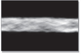
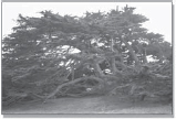
Figure 5-32: Original Background
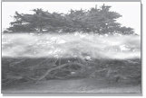
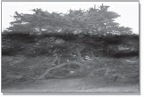
Figure 5-34: Scaled Background
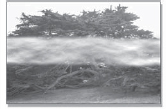
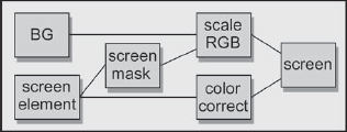
Figure 5-36: Flowgraph of Weighted Operation Screen
5.5.3 Multiply
The multiply operation simply multiplies two images together and is another matte-free way of combining two images. Like the screen operation, it simply mixes two images together mathematically without regard to which is on top. The multiply operation is analogous to projecting one image over the other, somewhat like putting a picture in a slide projector and projecting it over some object in the room. Of course, if you really did project a slide onto some object, the resulting projected image would appear quite dark. The reason is that you are not projecting it on a white reflective screen, but on some darker, poorly reflective and probably colored surface. The multiply operation behaves similarly.
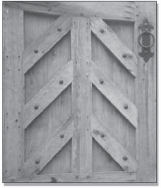


Figure 5-39: Multiplied Layers
Figure 5-37 and Figure 5-38 show an example of two images for multiplying. The ceramic tile painting in 5-38 is surrounded by a 100 percent white border in order to leave the wooden gate unmodified in this region. With a multiply operation, any 100 percent white pixels in one layer will leave the other layer unmodified. This is because the white pixels are treated as 1.0, and 1 times any pixel value results in the original pixel value. Note that the multiplied results are darker than either original layer, as we would expect from projecting a slide on a less than 100 percent white surface. We will deal with this issue momentarily.
The results of the screen operation universally lighten the images, and the results of the multiply operation universally darken them. The reason for this can be understood by taking an example. If you multiply 0.5 × 0.5 you get 0.25, a much smaller number. And so it is with all of the numbers between zero and 1.0.
Figure 5-40 illustrates two identical gradient images, A and B, multiplied together and the resulting darker image. It is actually a diagonally mirrored version of the screen operation graph in Figure 5-29. You could even think of the screen operation as an inverted multiply that results in a brighter output, whereas the regular multiply results in a darker output.

Figure 5-40: Results of Two Gradients Multiplied Together
5.5.3.1 Adjusting the Appearance
As with the screen operation, you cannot adjust the multiply operation. The two images are multiplied together and that's it. But, as with the screen operation, you can pre-adjust the images for better results. Normally you will want to brighten up the results, so the two plates need to be brightened before the multiply. You want to scale up the blacks and/or increase the gamma rather than adding constants to the plates. Adding constants will quickly clip the bright parts of each image.
Figure 5-41 illustrates the results of pre-adjusting the two plates before the multiply operation. Of course, you can also color correct the resulting image, but when working in 8 bits it is better to get close to your visual objective with precorrections, and then fine-tune the results. This avoids excessive scaling of the RGB values after the multiply operation, which can introduce banding problems with 8-bit images; 16-bit images would not suffer from banding problems.
An interesting contrast to the multiply operation is the semi-transparent composite of the same elements, shown in Figure 5-42. The composited results are a much blander “averaging” of the two images rather than the punchy and interesting blending you get with the multiply. Each of the two images retains much more of its identity with the multiply operation.
5.5.4 Maximum
Another matte-less image combining technique is the maximum operation (“Lighten” in Adobe Photoshop). The maximum node is given two input images, which it compares on a pixel by pixel basis. Whichever pixel is the maximum between the two images becomes the output. It is commonly used to combine mattes, but here we will use it to combine two color images. Who among us has not tried to composite a live action fire or explosion element over a background only to be vexed by dark edges? The fire element is, in fact, a poor source of its own matte.

Figure 5-41: Color Graded Layers Multiplied

Figure 5-42: Semi-Transparent Composite
The virtues of the maximum operation are that it does not need a matte and it usually produces very nice edges. The problem with the maximum operation is that it requires very specific circumstances to be useful. Specifically, the item of interest not only must be a bright element on a dark background, but that dark background must be darker than the target image with which it is to be combined. The basic setup can be seen starting with the fireball in Figure 5-43.
The fireball is on a dark background and the target image in Figure 5-44 is also a dark plate. When the two images are “max'd” together in Figure 5-45 the fireball comes through the target image wherever its pixels are brighter. There is no matte, so there are no matte lines, and even subtle detail such as the glow around the bottom of the fireball is preserved.
One problem you can have with the maximum operation is that there might be internal dark regions within the fireball that will become “holes” through which the target image can be seen. To fix this, a luminance matte can be generated from the fireball and then eroded to pull it well inside the edges. The original fireball can then be composited over the max'd image (Figure 5-45) to fill in the interior, somewhat like the soft comp/hard comp procedure we saw in Section 5.3.2. What you end up with is the nice edges of the maximum operation and the solid core of the composite operation.
The appropriate use for this operation is when the “hot” element is live action where you have no control over its appearance. If it is cgi or a painted element you do have control and can have the hot element placed over zero black for a screen operation or generate a matte for compositing. With a live action element you have to take what you are given and make it work. In addition to fire and explosion elements, the maximum operation can be used with photographed light sources, beams, or even lens flares—any bright live action element on a dark background.
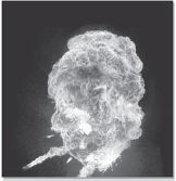
Figure 5-43: Fireball on a Dark Background

Figure 5-44: Dark Target Image
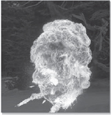
Figure 5-45: Fireball Max'd with Target Image

Figure 5-46: Paragliders Source Plate

Figure 5-47: Garbage Matted Source Plate

Figure 5-48: Paragliders Min'd into a Background
5.5.5 Minimum
The minimum operation (“Darken” in Adobe Photoshop) is, not surprisingly, the opposite of the maximum. When presented with two input images, it selects the darkest pixel between them as the output. This may not sound very exciting, but it can occasionally be very useful as another matte-less compositing technique. The setup for the minimum operation is that the item of interest is a dark element on a light background and the target image is also light—just the opposite of the setup for the maximum operation.
Take, for example, the paragliders in Figure 5-46. They are fairly dark, and the sky is fairly light, but there are dark regions near the bottom of the screen. To solve this little problem the plate has been garbage matted with a white surround in Figure 5-47. With the minimum operation the white surround becomes a “null” element that will not come through the target plate. The garbage matted version is then “min'd” with a background plate to produce the very nice composite in Figure 5-48.
Of course, the minimum operation suffers from all the same limitations as the maximum operation in that you must have suitable elements, you may have to pull a matte to fill in the core, and you may have to garbage matte the item of interest to clear the surround. However, when it works it can be a very elegant solution to a tough problem.