
![]()
Introduction to Pure Data
Pure Data, a.k.a. Pd, is a visual programming language and environment for audio and visuals. It is open source and it was made by Miller Puckette during the 1990s. Visual programming means that instead of writing code (a series of keywords and symbols that have a specific meaning in a programming language), you use a graphical interface to create programs, where in most cases, a “box” represents a certain function, and you connect these “boxes” with lines, which represent patch cords on analog audio devices. This kind of programming is also called data flow programming because of the way the parts of a program are connected, which indicates how its data flows from one part of the program to another.
Visual programming can have various advantages compared to textual programming. One advantage is that a visual programming language can be very flexible and quick for prototyping, where in many textual programming cases, you need to write a good amount of lines of code before you can achieve even something simple. Another advantage is that you can say that visual programming is more intuitive than textual programming. When non-programmers confront visual code, it’s very likely that they will get a better idea as to what this code does than when confronting textual code. On the other hand, there are also disadvantages and limitations imposed by visual programming. These are technical and concern things like DSP chains, recursion, and others, but we won’t bother with these issues in this book, as we’ll never reach these limits. Nevertheless, Pd is a very powerful and flexible programming language used by professionals and hobbyists alike around the world.
Throughout this book, we’ll use Pd for all of our audio and sequencing programming, always in combination with the Arduino. The Arduino is a prototyping platform used for physical computing (among other things), which enables us to connect the physical world with the world of computers. A thorough introduction to Arduino is given in Chapter 2. This chapter is an introduction to Pd, where we’ll go through its basics, its philosophy, as well as some general electronic music techniques. If you are already using Pd and know its basics, you can skip this chapter and go straight to the next one. Still, if you’re using Pd but have a fuzzy understanding on some of its concepts, you might want to read this chapter. Mind that the introduction to Pd made in this chapter is centralized around the chapters that follow, and even though some generic concepts will be covered, it is focused on the techniques that will be used in this book’s projects.
In order to follow this chapter and the rest of this book, you’ll need to install Pd on your computer. Luckily, Pd runs on all three major operating systems: OS X, Linux, and Windows. You can download it for free from its web site at https://puredata.info/. You will find two version of Pd: vanilla and extended. Pd-vanilla (simply Pure Data) is the “vanilla” version of Pd, as its nickname states. It’s the version made and maintained by Miller Puckette, and it consists of the core of Pd. Most of the things we’ll be doing in this book can be made with vanilla, but Pd-extended adds some missing features to Pd that we will sometimes use. For example, the communication between Pd and Arduino is achieved with Pd-extended and not vanilla. Of course, you can add these features to vanilla, but it’s beyond the scope of this book to explain how to do this, so we’ll be using Pd-extended in all of our projects. Find the version for your OS and install it on your computer before you go on reading.
By the end of this chapter, you’ll be able to
- understand how a Pd program works
- create small and simple programs in Pd
- find help in the Pd environment
- create oscillators in Pd
- make use of existing abstractions in Pd and create your own
- realize standard electronic music techniques in Pd
Pd Basics: How It Works
Pd consists of several elements that work together to create programs. The most basic elements are the object and the message. An object is a function that receives input and gives output. Figure 1-1 shows the osc~ Pd object.
![]()
Figure 1-1. A Pd object
This specific object is a sine wave oscillator with a 440-hertz (Hz) frequency. There’s no need to understand what this object does; we’ll go through that in a bit. There are a few things we need to note. First of all, there is specific text inside the object box, in this case “osc~ 440”. “osc” stands for oscillator, and the ~ (called the tilde) means that this object is a signal object. In Pd, there are two types of objects: signal and control. A signal object is a function that deals with signals (a digital form of an electric signal). A signal object will run its function for as long as the audio is on (the audio is also called the DSP, which stands for digital signal processing, or the DAC, digital-to-analog converter). A control object is independent of audio and runs its function only when it is told to. We’ll get a better picture of the difference between the two as we go. The last part of the text, “440”, is called an argument. This is the data that a function receives, and we provide it as an argument when we want to initialize an object with it. It is not necessary to provide an argument; when there’s no argument in an object, the object is initialized with the value(s) of zero (0).
The second main element in Pd is the message, which is shown in Figure 1-2.
![]()
Figure 1-2. A Pd message
It is a little bit different from the object, because on its right side, it is indented, and it looks a bit like a flag. The message delivers data. There’s no function here, only the data we write in the message (sometimes referred to as a message box). One thing the object and the message have in common is the inlets and the outlets. These are the little rectangles on the top and the bottom, respectively, of the object and the message. All messages have the same form, no matter what we type in them. They all have one inlet to receive data and one outlet to provide the data typed in them. The objects differ, in the sense that each object has as many inlets as it needs to receive data for its function, and as many outlets as it needs to give the output(s) of the function. With the osc~ object, we can see that it has two inlets and one outlet. The left inlet and the outlet are different than the right inlet. Their rectangle is filled, whereas the right inlet has its rectangle blank, like the message does. The filled inlets/outlets are signal inlets/outlets and the blank ones are control inlets/outlets. Their differences are the same as the signal and control objects. Note that a signal object can have control inlets/outlets, but a control object cannot have signal inlets/outlets.
Objects and messages in Pd are connected with lines, which we also simply call connections. A message connected to the osc~ object is shown in Figure 1-3.
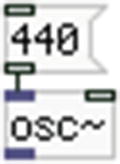
Figure 1-3. A message connected to an object
A connection comes out the outlet of the message and goes to the inlet of the object. This way we connect parts of our programs in Pd.
Our First Patch
Now let’s try to make the little program (programs in Pd are called patches, which is what I will call them from now on). Launch Pd like you launch any other application. When you launch it, you get a window that has some comments in it. Don’t bother with it; it is just some information for some features it includes. This is the Pd window, also called the Pd console, and you can see it in Figure 1-6. It is very important to always have this window open and visible, because we get important information there, like various messages printed from objects, error messages, and so forth.
Go to File ![]() New to create a new window. You will get another window that is totally empty (don’t make it full-screen because you won’t be able to see the Pd console any more). Note that the mouse cursor is a little hand instead of an arrow. This means that you are in Edit Mode, so you can edit your patch. In this window, we will put our objects and messages. In this window’s menu, go to Put
New to create a new window. You will get another window that is totally empty (don’t make it full-screen because you won’t be able to see the Pd console any more). Note that the mouse cursor is a little hand instead of an arrow. This means that you are in Edit Mode, so you can edit your patch. In this window, we will put our objects and messages. In this window’s menu, go to Put ![]() Object (in OS X there’s a “global” menu for the application; it’s not on every window). This will create a small dotted rectangle that follows the mouse. If you click once, it will stop following the mouse. Inside the rectangle, there’s a blinking cursor. This means that you can type in there. For this patch, you will type osc~.
Object (in OS X there’s a “global” menu for the application; it’s not on every window). This will create a small dotted rectangle that follows the mouse. If you click once, it will stop following the mouse. Inside the rectangle, there’s a blinking cursor. This means that you can type in there. For this patch, you will type osc~.
After you type this, click anywhere in the window, outside the object, and you’ll see your first Pd object, which should look like the one shown in Figure 1-1. (Note the shortcut for creating objects; it’s Ctrl+1 for Linux and Windows, and Cmd+1 for OS X. We’ll be using the shortcut for creating objects for now on). Now go to Put ![]() Message (the second choice in the menu, with the Ctrl/Cmd+2 shortcut). This will create a message. Place it somewhere in the patch, preferably above the object. Once you’ve already placed a message or an object in a patch, to move it, you need to select it by dragging. You can tell that is has been selected because its frame and text is blue, as shown in Figure 1-4.
Message (the second choice in the menu, with the Ctrl/Cmd+2 shortcut). This will create a message. Place it somewhere in the patch, preferably above the object. Once you’ve already placed a message or an object in a patch, to move it, you need to select it by dragging. You can tell that is has been selected because its frame and text is blue, as shown in Figure 1-4.
![]()
Figure 1-4. A selected message
If you click straight into the message or object, it will become editable, and it will be blue like in Figure 1-4, but there will also be a blue rectangle inside it, like in Figure 1-5. When an object or message looks like the one in Figure 1-5, you cannot move it around but only edit it.
![]()
Figure 1-5. An editable message

Figure 1-6. The Pd console
Type 440 and click outside it. To connect the message to the object, hover the mouse above the outlet of the message (on its lower side). The cursor should change from a hand to a circle and the outlet should become blue (on Linux, the cursor changes from a hand to an arrow, with a small circular symbol next to it). Click and drag. You will see a line coming out the outlet of the message. When holding the mouse click down, if you hover over the left inlet of the object, the cursor will again become a circle and the inlet will become blue. Let go of the mouse click, and the line will stay between the message and the object. You have now made your first connection.
What we have until now is a patch, but it doesn’t really do anything. We need to put at least one more object for it to work. Again, put an object in your patch (preferably with the shortcut instead of using the menu) and place it below the [osc~] object (using square brackets indicates a Pd object when Pd patches are explained in text). This time, type dac~. This object has two inlets and no outlets. This is actually your computers’ left and right speakers. Connect the outlet of [osc~] to both inlets of [dac~], the same way you connected the message to [osc~]. Your patch should look like the one in Figure 1-7.

Figure 1-7. A simple Pd patch
You might notice that the connections that come out from [osc~] are thicker than the one coming out from the message. These are signal connections, whereas the thin one is a control connection. The difference is the same as with signal/control objects.
Now we have a fully functional patch. In order to make it work, we need to take another two steps. First, we need to get out of Edit Mode. Go to the Edit menu and you’ll see Edit Mode; it is ticked, which means that you are in this mode. If you click it, the cursor will turn from a little hand to an arrow. This means that you are no longer in Edit Mode and cannot edit the patch, but you can interact with it. If you go to the Edit menu again, you’ll see that Edit Mode is not ticked anymore. From now on, we’ll use the shortcut for Edit Mode, which is Ctrl/Cmd+E. The last thing you need to do to activate the patch is to turn on the DSP. Go to Media ![]() DSP On (Ctrl+/or Cmd+/). On the Pd console, there is a DSP tick box. To turn on the DSP, select the tick box; DSP becomes green, as shown in Figure 1-8. When the DSP is on, all signal objects are activated. Make sure to put your computer’s volume at a low level before you turn the DSP on, as it might sound rather loud.
DSP On (Ctrl+/or Cmd+/). On the Pd console, there is a DSP tick box. To turn on the DSP, select the tick box; DSP becomes green, as shown in Figure 1-8. When the DSP is on, all signal objects are activated. Make sure to put your computer’s volume at a low level before you turn the DSP on, as it might sound rather loud.

Figure 1-8. DSP on indication on Pd’s console
Even though you turned on the DSP, you still hear nothing. Hover the mouse over the message (you’ll see the cursor arrow change direction, which means that you can interact with the element you hover your mouse over) and click. Voila! You have your first functional Pd patch! This is a very simple program that plays a sine wave at a 440 Hz frequency.
Before getting overly excited, it’s good practice to save your first patch. Before you do that, you might want to turn the DSP off by going to Media ![]() DSP Off (Ctrl/Cmd+.) Now the DSP tick box should be unticked. Saving a patch is done the same way that you save a text file. Go to File
DSP Off (Ctrl/Cmd+.) Now the DSP tick box should be unticked. Saving a patch is done the same way that you save a text file. Go to File ![]() Save As... (Shift+Ctrl/Cmd+S) and a dialog window will open. Here you can set a name for your patch (that could be my_first_patch) and a place to save it. If you haven’t done so yet, create a folder somewhere in your computer (a good place is Documents/pd_patches, for example, definitely not the Program Files folder) and click Save. It’s good practice to avoid using spaces both in Pd patch names and folders used by Pd, as it’s pretty difficult to handle them. It’s better to use an underscore (_) instead. Also, notice the file extension created by Pd, which is .pd (not too much of a surprise . . .). These are the files that Pd reads.
Save As... (Shift+Ctrl/Cmd+S) and a dialog window will open. Here you can set a name for your patch (that could be my_first_patch) and a place to save it. If you haven’t done so yet, create a folder somewhere in your computer (a good place is Documents/pd_patches, for example, definitely not the Program Files folder) and click Save. It’s good practice to avoid using spaces both in Pd patch names and folders used by Pd, as it’s pretty difficult to handle them. It’s better to use an underscore (_) instead. Also, notice the file extension created by Pd, which is .pd (not too much of a surprise . . .). These are the files that Pd reads.
Now that we’ve saved our first patch, let’s work on it a bit more. Go back to Edit Mode (Ctrl/Cmd+E) to edit your patch. The cursor should again turn to a little hand. Now we’ll replace the message with another element of Pd, the number atom. First, we’ll need to delete the message. To do this, drag your mouse and select it, the same way you select it to move it around. Hit Backspace and the message (along with its connections) will disappear. Go to Put ![]() Number (Ctrl/Cmd+3) and the number atom will be added to your patch, which is shown in Figure 1-9.
Number (Ctrl/Cmd+3) and the number atom will be added to your patch, which is shown in Figure 1-9.
![]()
Figure 1-9. A number atom
Connect its outlet to the left inlet of [osc~] (it actually replaces the message) and get out of Edit Mode. Turn the DSP on and again you’ll hear the same tone as before. This is because [osc~] has saved the last value it received in its inlet, which was 440. Click the number atom and type a number (preferably something different than 440) and hit Return (a.k.a. Enter). You have now provided a new frequency to [osc~] and the pitch of the tone you hear has changed to that. Another thing you can do with number atoms is drag their values. Click the number and drag your mouse. Dragging upward will increase the values and dragging downward will decrease them. You should hear the result instantly. When done playing, turn off the DSP and save this patch with a different name from the previous one.
The Control Domain
Our next step will be dealing with the control domain. As mentioned, the control objects are independent of the DSP and run their functions only when they are instructed to do so, regardless of the DSP being on or off. Let’s create a simple patch in the control domain. Let’s open a new window and put an object in it. Inside the object type +. This is a simple addition object. It has two inlets and one outlet, because it adds two numbers and gives the result of the addition. Now put three number atoms and connect two of them to each inlet of [+ ] and the outlet of [+ ] to the inlet of the third number. Make sure that your patch is like the one in Figure 1-10.
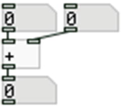
Figure 1-10. A control domain patch
Go out of the Edit Mode (from now on we’ll refer to this action as “lock your patch”) and click the top-right number. Type a number and hit Return. Doing this gives no output. Providing a value to the top-left number, will give the result of the addition of the two values, which is displayed on the bottom number atom. What we see here are the so-called cold and hot inlets in action. In Pd, all control objects have cold and hot inlets. No matter how many inlets they have (unless they have only one), all of them but the far left are cold. This means that providing input to these inlets will not give any output, but will only store the data in the object. The far left inlet of all control objects is hot, which means that providing input to that inlet will both store the data and give output. This is a very important rule in Pd, as its philosophy is a right-to-left execution order. It might take a while to get used to this, and not bearing it in mind might give strange results sometimes; but as soon as you get the grasp of it, you’ll see that it is a very reasonable approach to visual programming.
Execution Order
Before moving on to some other very important aspects of Pd, I should talk a bit more about the order of execution, since you saw a small example earlier. In a new patch, put a number atom and put an object below it. Type * inside the object. This is a multiplication object, which works in a way similar way to the addition object you saw. Connect the number to both inlets of [* ], but first connect it to the left inlet of [* ] and then to the right one. Put another number and connect the outlet of [* ] to the inlet of the new number. You should have the patch shown in Figure 1-11.
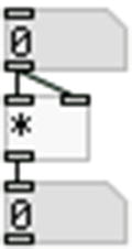
Figure 1-11. A fan out connection
As you can imagine, this patch gives the square of a given number by multiplying it to itself. Lock your patch and type the number 2 in the number atom. What you would expect to receive is 4, right? But instead, you got 0. Now type 3. Again, you would expect to get 9, but you got 6. Now type 4. Instead of 16, you got 12.
Even though I said that Pd executes everything from right to left, another rule is that execution will follow the order of connection. That means that if you connect the top number atom to the left inlet of [* ] first, and then to the right one, whatever value you provide through the number atom will first go to the left inlet of [* ] and then to the right. But I’ve already mentioned that all left inlets in all control objects are hot, and all the rest are cold. So what happens here is that when we gave the number 2 to [* ], it went first to the left inlet and we immediately received output. That output was the number provided in the left inlet, and whatever other value was stored in [* ]. But we hadn’t yet stored any value, so [* ] contained 0,1 and gave the multiplication 2 * 0 = 0. Immediately after this happened, the number 2 went to the right inlet of [* ] and was stored, but gave no output, as the right inlet is cold. The next time we gave input to [* ], we sent the number 3. Again, we got the same behavior. [* ] first gave the multiplication of 3 by the number already stored, which was 2 from the previous input, so we got 3 * 2 = 6; and then the number 3 was stored in [* ] without giving output. The same thing happened with as many numbers we provided [* ] with.
If we had connected the number atom to the right inlet of [* ] first and then to the left one, things would have worked as expected. But connecting one element to many can be confusing and lead to bugs, which can be very hard to trace. In order to avoid that, we must force the execution order in an explicit way. To achieve this, we use an object called trigger. Disconnect the top number atom from [* ] and put a new object between them. In it, type t f f. “t” is an abbreviation for trigger and “f” is an abbreviation for float. A float in programming is a decimal number, and in Pd, all numbers are considered decimals, even if they are integers. [t f f] has one inlet (which is hot) and two outlets. Connect the top number atom to the inlet of [t f f] and the outlets of [t f f] to the corresponding inlets of [* ]. You should have a patch like the one shown in Figure 1-12.

Figure 1-12. Using [trigger] instead of fan out
[t f f] follows Pd’s right-to-left execution order, no matter which of its inlets gets connected first. Now whichever number you type in the top number atom, you should get its square in the lower number. This technique is much safer than the previous one and it is much easier for someone to read and understand. By far, it’s preferred over connecting one outlet to many inlets without using trigger, a technique called fan out.
Bang!
It’s time to talk about another very important aspect of Pd, the “bang.” The bang is a form of execution order. In simple terms, it means “do it!”. Imagine it as pressing a button on a machine that does something—the elevator, for example. When you press the one and only button to call the elevator, the elevator will come to your floor. In Pd language, this button press is called a bang. In order to understand this thoroughly, we’ll build a simple patch that counts up, starting from zero. Open a new window and put two objects. In one of them, type f, and in the other + 1 (always use a space between object name and argument). “f” stands for float, as in the case of [trigger], and [+ 1] is the same as [+ ] we have already used, only this time it has an argument, so we don’t need to provide a value in its right inlet. Whatever value comes in its left inlet will be added to 1 and we’ll get the result from its outlet. Connect these two objects in the way shown in Figure 1-13.

Figure 1-13. A simple counter mechanism
Take good care of the connections. [f ] connects to the left inlet of [+ 1], but [+ 1] connects to the right inlet of [f ]. If you connect [+ 1] to the left inlet of [f ], then you’ll have connected each object to the hot inlet of the other. In this case, as soon as you try to do anything with this, you’ll get what is called a stack overflow, as this will cause an infinite loop, since there will be no mechanism to stop it.
Above these two objects put a message and type bang in it. Connect its outlet to the inlet left of [f ]. Lastly, put a number atom below the two objects and connect the outlet of [f ] to it. You should have the patch in Figure 1-14.
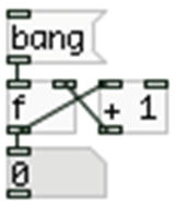
Figure 1-14. A simple Pd counter
Note that, even though in the previous section I mentioned the importance of using [trigger], here we’re connecting [f ] to two objects (one object and one number atom) without using [trigger]. This specific kind of patch is one of the very rare cases where execution order doesn’t really matter, so we can omit using [trigger]. Still, in most cases it is really not a good idea not to use it.
What we have now created is a very simple counter that counts up from zero (it starts from zero because we haven’t provided any argument to [f ], and as already stated, no argument defaults to zero). [f ] will go to [+ 1], which will give 0 + 1 = 1. This result will go to the right inlet of [f ], meaning that the value will only be stored and we’ll get no output. The value that comes out of [f ] will also go to the number atom, where it will be displayed. The next time [f ] will throw its value, it will be 1, which will go to [+ 1], which will give 1 + 1 = 2, which will be stored in [f ], and 1 will be displayed in the number atom, and so on.
For [f ] to output its value, it must receive some kind of trigger. This is where the “bang” comes in. Lock your patch and click the message. The first time you’ll see nothing because [f ] will output zero, but the number atom displays zero by default. Hit the message again and you’ll see the value 1 in the number atom. The next time you hit the “bang” message, you’ll see 2, and so on.
This is how we create a simple counter, which a very valuable tool in programming—for example, when building a sequencer, which we’ll do in Chapter 4. We’ve also seen bang in action, a very important aspect of Pd.
In programming, one common element between different languages is the comment. A comment is just this, a comment. It’s there to provide information about some features of a program or a part of it. Pd is no different when it comes to comments. In a new patch, go to Put ![]() Comment (Ctrl/Cmd+5) and the word “comment” will appear, following your mouse. As with all other elements, click so that it stops following the mouse. By clicking, you’ll also see a blue rectangle around the comment. This means that you can edit it. Go ahead and type anything you want. Figure 1-15 shows a Pd comment.
Comment (Ctrl/Cmd+5) and the word “comment” will appear, following your mouse. As with all other elements, click so that it stops following the mouse. By clicking, you’ll also see a blue rectangle around the comment. This means that you can edit it. Go ahead and type anything you want. Figure 1-15 shows a Pd comment.
![]()
Figure 1-15. A Pd comment
From the early stages in programming learning up to professional programming, it is typical to see comments, which are extremely helpful. Comments help others understand your programs more easily, but also help you to understand your own programs when you come back to them some time after you’ve made them. With comments, we covered the most basic and useful elements of Pd.
Getting Help
Pd is a programming language that is very well documented. Even though it’s open source, and nobody gets paid for creating it, maintaining it, developing it, or documenting it, it still has a great amount of documentation. When we say documentation, we don’t really mean tutorials in its usual sense, but help files, which themselves are some kind of short tutorials. Every element, like the object, the message, and so forth in Pd has a help file, which we call a help patch. To get to it, all you need to do is right-click the element. You get a menu with three choices: Properties, Open, and Help. The first two are very likely to be grayed out, so you can’t choose them, but Help is always available. Clicking it will open a new patch, which is the help patch of the element you chose. All elements but the object have one help patch, as they do something very specific (the message, for example, delivers a message, and that’s all it does). But the object is a different case, as there are many of them in Pd. So, depending on the object you choose (which is defined by the text in it), you’ll get the help patch for that specific object. For example, [osc~] has a different help patch than [dac~].
In a patch, put an object ([osc~] for instance), a message (no need to type anything in it), a number atom, and a comment (also no need to type anything), and right-click each of them and open their help patches. In there, there’s text (actually comments) describing what the element does, and providing examples and other information. Don’t bother to read everything for now, you’re just checking it to get the hang of finding and using help patches. You need to know that you can copy and use parts or the whole patch into your own patch. Go ahead and play a bit with the examples provided, and if you want, click the Usage Guide link on the bottom left. This will open a help patch for help patches, describing how a help patch is structured to get a better understanding of them. Mind that objects starting with pd (for example, [pd Related_objects]) are clickable and doing so (in a locked patch) will open a window. This is called a subpatch, which we’ll cover further on.
Lastly, right-clicking a blank part of a patch, will open the same menu, but this time Properties is selectable. You won’t select it now, but instead click Help. This will open a help patch with all the vanilla objects (you might get some red messages in Pd’s console, called error messages, but it’s not a problem). If you want, you can go through these, but don’t bother too much, as it might become a bit overwhelming. By using Pd more and more, you get to know the available objects or how and where to look for what one needs.
GUIs
The next step is the GUI. GUI stands for graphical user interface. In computers, GUIs are very common. Actually, Pd itself runs as GUI and your computer system too (most likely). All the windows you open from various programs are considered GUIs. This approach is usually much preferred over its counterpart, the CLI (command-line interface), where the user sees only text and interacts with it in a terminal window, for example.
Even though Pd itself runs as GUI (since it is visual and not textual) there are some elements of it that are considered to be its GUIs (the elements covered so far, but the number atom are not GUIs). If you click the Put menu, the second group of elements contains GUIs: the Bang, the Toggle, the Number2, and so forth. The ones we’ll use most are the bang, the toggle, the sliders, and the radios, which you can see in Figure 1-16.

Figure 1-16. The bang, the toggle, the sliders, and the radios
Open a new patch and put a bang from the Put menu (Shift+Ctrl/Cmd+B). This is the graphical representation of the [bang] (a Pd message in textual form starts with an opening square bracket and ends with an opening parenthesis, imitating the way it looks in Pd). The Bang is clickable and it outputs a bang. Right-click it and open its help patch (here the Properties are not grayed out and are selectable, but we won’t delve into this for now). On the top-right of the help patch, there’s an object [x_all_guis . . .]. Click it and a new window will open with all the GUIs in Pd. From there you can right-click each and check its help patch to see what it does. Focus on the GUIs that we’ll typically use, which I’ve already mentioned. Let’s talk a bit about these.
We’ve already covered the Bang, so let’s now talk about the Toggle. The Toggle functions like a toggle switch; it’s either on or off. It’s a square, and when you click it (in a locked patch), an X appears in it. That’s when it’s on. When there’s no X in it, it’s off. By “on” and “off” here, I mean 1 and 0. What the Toggle actually does is output a 1 and a 0 alternately when clicking it, and we can tell what it outputs by the X that appears in it.
The Slider (Vslider stands for vertical slider and Hslider for horizontal slider) is a GUI imitating the slider in hardware; for example, in a mixing desk. Clicking and dragging the small line in it outputs values from 0 to 127 by default, following the range of MIDI; but this can be changed in its properties. You can get these values from its outlet.
The Radio (again Vradio and Hradio stand for vertical and horizontal) works a bit like a menu with choices (like the one that appears when you right-click a Pd element). Only instead of text, it consists of little white squares next to each other, and clicking them outputs a number starting from 0 (clicking the top of the Vradio will output 0, clicking the one below will output 1, and so forth). The Hradio counts from left to right. You can tell which one is currently clicked by a black square inside it. It doesn’t really sound like a menu, but remember that Pd is a programming language, meaning that we need to program anything we want it to do. This way, provided a very simple GUI that outputs incrementing values, we can use it to create something more complex out of it. We’ll see it in action in the interface building projects in this book. We’ve now covered the GUIs that we will use and we can move on.
Pd Patches Behave Like Text Files
When we edit a Pd patch, we can use features that are common between text editing programs. This means that we can choose a certain part of the patch (by clicking and dragging in Edit Mode), copy it, cut it, duplicate it, paste it somewhere else in the patch, or in another patch. If you click the Edit menu, you’ll see all the available options.
The ones we’ll mostly use in this book are Copy (Ctrl/Cmd+C), Paste (Ctrl/Cmd+V), Cut (Ctrl/Cmd+X), and Duplicate (Ctrl/Cmd+D). Actually, a Pd patch is text itself. If you open any patch in a text editing program, you’ll see its textual form. The first patch we created in this chapter, with the [440] message and [osc~] and [dac~], looks like what’s shown in Figure 1-17.

Figure 1-17. A Pd patch in its textual form
Even though this is pretty simple, you don’t really need to understand it thoroughly, as we’re not going to edit patches in their textual form in the course of this book. Still, it’s good to know what a Pd patch really is.
Now that we’ve covered the real basics of Pd, and you know how to create patches, let’s look at some sound generators that we will use in later chapters. First, I need to explain what an oscillator is. In analog electronics, it is a mechanism that creates certain patterns in an electrical current, which is fed to the sound system, causing the woofers of the speakers to vibrate in that pattern, thus creating sound. In digital electronics, this mechanism consists of very simple (or sometimes more complex) math operations (here we’re talking about multiplication, addition, subtraction, and division, nothing else) that create a stream of numbers that is fed to the sound card of a computer, turning this number stream to an electrical current. From that point on, up to the point the electrical current reaches the sound system’s speakers, everything is the same between analog and digital electronics. The patterns that the oscillators create are called waveforms, because sound is perceived in auditory waves.
There are four standard waveforms in electronic music, which we will create in this section. These are the sine wave, the triangle, the sawtooth, and the square wave. They are called like this because of the shapes they create, which you can see in Figure 1-18.

Figure 1-18. The four standard oscillator waveforms: the sine wave, the triangle, the sawtooth, and the square wave
Some other audio programming environments have classes for all these waveforms, but Pd has an object only for the first one, the sine wave. Some consider this to be a bad thing, but others consider it to be good. Not having these oscillators available means that you need to build them yourself, and this way you learn how they really function, which is very important when dealing with electronic music. The object for the sine wave oscillator is [osc~], which you’ve already seen, so we’re not going to talk about it here.
Before moving on to the next waveform, we need to talk about the range of digital audio. Audio in digital electronics is expressed with values from –1 to 1 (remember, a digital signal is a stream of numbers representing the amplitude of an electric signal). In the waveforms in Figure 1-18, -1 is expressed by the lowest point in the vertical axis, and 1 by the highest (waveforms are represented in time, which lies at the horizontal axis). Paralleling this range to the movement of the speaker’s woofer, –1 is the woofer all the way in, 1 is the woofer all the way out, and 0 is the woofer in the middle position (this is also the position when it’s receiving no signal). Figure 1-19 represents these positions of the woofer by looking at it from above.

Figure 1-19. The speaker’s woofer’s positions and their corresponding digital values
Making a Triangle Wave Oscillator
Now to the next wave form, which is the triangle. We will create this with simple objects. The driving force for every oscillator (and other things we’ll build along the way) is the [phasor~]. [phasor~] is a rising ramp that looks like the sawtooth wave form, only it outputs values from 0 to 1. To create a triangle out of this, we need a copy of [phasor~]; but instead of rising, we need it to be falling from 1 to 0. To achieve this, we must multiply [phasor~]’s output by –1 and add 1. This is very simple math if you think about it. If you multiply [phasor~]’s initial value, which is 0, by –1, you’ll get 0, and if you add 1 you’ll get 1. If you multiply [phasor~]’s last value, which is 1, by –1, you’ll get -1, and if you add 1, you’ll get 0. All the values in between will form the ramp from 1 to 0. Mind, though, that we are now in the signal domain and all the objects we’ll use are signal objects. So for multiplying, we’ll use [*~ ] and for adding we’ll use [+~ ].
Once we have the two opposite ramps, we’ll send them both to [min~]. This object takes two signals and outputs the minimum value of the two. The two ramps we have intersect at the value 0.5 during their period (a period in a wave form is one time its complete shape, like the preceding wave form images). For the first half of the period, the rising [phasor~] is always less than the falling one (the rising one starts from 0 and the falling from 1), so [min~] will output this. For the second half of the period, the falling [phasor~] will be less than the rising one, so [min~] will output that. What [min~] actually gives us is a triangle that starts from 0, goes up to 0.5, and comes back to 0. Figure 1-20 illustrates how this is actually achieved.
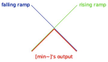
Figure 1-20. Getting a triangle out of two opposite ramps
As I’ve already mentioned, the range of oscillators is from –1 to 1. This is 2 in total. So, multiplying the output of [min~] by 4, will give us a triangle that goes from 0 to 2. Subtracting 1, will bring it to the desired range. These last two actions—the multiplication and the subtraction—are called scaling and offset, respectively. So, our triangle oscillator patch should look the patch in Figure 1-21.
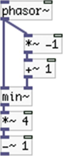
Figure 1-21. The triangle oscillator Pd patch
Connect a number atom to [phasor~] to give it a frequency (lock your patch before trying to type a number into the number atom) and place a [dac~] and connect [-~ 1] to it. Turn on the DSP and listen to this wave form. Compare its sound to the sound of [osc~]. The triangle wave form is brighter than the sound of the sine wave, which is because it has more harmonics than the sine wave. Actually, the sine wave has no harmonics at all, and even though it is everywhere in nature, you can only reproduce it with such means, as you can’t really isolate it in nature.
Note that execution order doesn’t apply to the signal domain, because signal objects calculate their samples in blocks, and they have received their signals from all their inlets before they go on and calculate the next audio block.
The next waveform we’ll build is the sawtooth. This one is very easy, since we’ll use [phasor~], which is itself a sawtooth that goes from 0 to 1, instead of –1 to 1. All we need to do here is correct its range, meaning apply scaling and offset. Since [phasor~] has a value span of 1, and oscillators have a value span of 2, we have to multiply its output by 2; so now we get a ramp from 0 to 2. Subtracting 1 gives us a ramp from –1 to 1, which is what we essentially want. The patch is illustrated in Figure 1-22.

Figure 1-22. The sawtooth oscillator Pd patch
Supply [phasor~] with a frequency and connect [-~ 1] to [dac~] to hear it. Compared to the two previous oscillators, this one has even more harmonics, which you can tell by its brightness; its sound is pretty harsh.
Making a Square Wave Oscillator
Finally, let’s build the last wave form, the square wave. This oscillator is alternating between –1 and 1, without any values in between. Again, we’ll use [phasor~] to build it. Now we’ll send [phasor~] to a comparison object, [<~ ], which compares if a signal has a smaller value than another one, or a value smaller than its argument (if one is provided). If the value is smaller, [<~ ] will output 1, else it will output 0. Connecting [phasor~] to [<~ 0.5] (don’t forget the space between the object name and the argument), will give 1 for the first half of [phasor~]’s period, and 0 for the other half, because [phasor~] goes from 0 to 1, linearly. Multiplying this by 2 and subtracting one will give an alternating 1 and –1, which is what the square wave oscillator is.
This oscillator has one more control feature, which is how much of its period it will output a 1, and how much it will output a 0 (for example, it can output a 1 for 75% of its period and a 0 for the rest 25%, or vice versa, or any such combination). This is called the duty cycle, which is easy to make in Pd. All you need to do is control [<~ ] with a value that ranges from 0 to 1 (actually from something over 0, like 0.01, to something less than 1, like 0.99). If you connect a number atom to the right inlet of [<~ 0.5] you’ll override the argument with whatever number you provide (mind that the right inlet of [<~ 0.5] is a control inlet, and that is because you have provided an argument. If you create the object without an argument, both its inlets will be signal inlets). Your patch should look Figure 1-23.

Figure 1-23. The square wave oscillator Pd patch
Try some different values by typing into the number atom (in a locked patch), always staying between 0.01 and 0.99. You can also hold down the Shift key and click and drag the number atom. This way, it will scroll its values with two decimal places.
Mind that it is possible to create the same oscillator with [>~ ] instead of [<~ ]; the only difference is that it will first output –1 and then 1, but that’s a difference that is not recognizable by the human ear. Comparing this oscillator to the others, we see that this one also has a lot of harmonics, as its sound is very bright.
We have now created the four basic oscillators of electronic music. Their raw continuous sound might not be very musical or inspiring, but the way we’ll use them in some of this book’s projects will be quite different and will provide more musical results.
Using Tables in Pd
The next feature we’re going to look at is tables. You’ll learn how to use them in Pd. You learned about tables in school math; a table stores values based on an index. In Pd, this is either called a table, and you can create it with [table], or array, which we can put from the Put menu. Open a new window and go to Put ![]() Array (there’s no shortcut for this one). A properties window will open, where you can set its name, its size, whether you want to save it contents, the way to draw its contents, and whether to put the array in a new or in the last graph. From these options, you’ll only deal with the first three. For now, you can keep the default name, which is array1. You’ll also keep the size for now, which is 100, but you’ll untick the Save contents field, because we don’t care to save whatever you’ll store in it.
Array (there’s no shortcut for this one). A properties window will open, where you can set its name, its size, whether you want to save it contents, the way to draw its contents, and whether to put the array in a new or in the last graph. From these options, you’ll only deal with the first three. For now, you can keep the default name, which is array1. You’ll also keep the size for now, which is 100, but you’ll untick the Save contents field, because we don’t care to save whatever you’ll store in it.
Click OK and you’ll see a graph in your patch. If you move it, you’ll also see its name projected on top of it, looking like the one shown in Figure 1-24.

Figure 1-24. A Pd array
Inside the array’s window, there’s a straight line, right in the middle, spanning from left to right. These are the values stored in the array, all of which are 0 for now. The values in an array are graphed in the Y axis and the indexes in the X axis. Indexes start counting from 0 and go from left to right. In our case, the last index is 99, as we have an array of size 100 and the first index is 0.
There are a few ways to store values in an array. The simplest one is to draw values by hand. Lock you patch and hover the mouse over the line in the middle of the array. Click and drag (both up and down, as well as right and left) and you’ll see that the line follows the mouse. This way is not very useful because you generally want to store certain patterns in arrays that are actually impossible to draw by hand.
Another way to store values is by using [tabwrite], where “tab” stands for table. This object has two inlets and no outlet. The right inlet sets the index and the left sets the value. It also takes an argument, which is the name of the array to write to. Put a [tabwrite array1] to your patch and connect a number atom to each inlet. Lock your patch and store a value to an index; for example, store 0.75 to index 55 (indexes are always integers). Mind to first provide the index to the right inlet, and then the value—again, the right to left execution order and hot and cold inlets apply. You should immediately see the dot at the 55th place jump to the value 0.75 (a bit lower than the upper part of the frame). To double-check it, put a [tabread array1], which reads values from an array. This one has one inlet and one outlet. In the inlet. you provide an index and it spits the value at that index out its outlet. Give it the value 55 and it should give 0.75.
All of this isn’t likely very intuitive and the point might seem a bit hidden. Let’s look at another way to use arrays. Right-click Array and click Properties. Now you get two windows, but we only care about the first one. Change the size of the array to 2048, click OK, and close both of these windows (whatever values we’ve already stored will shrink to the right, as there are now in the very first indexes). Copy one of the oscillator patches (the triangle, for example) built in the previous section, but instead of [dac~] at the bottom, put [tabwrite~ array1] (mind the tilde that makes it different from [tabwrite array1]). Connect a number atom to [phasor~] and a bang (Shift+Ctrl/Cmd+B) to [tabwrite~ array1] (this object has one inlet only and it takes both signals and bangs). Figure 1-25 shows what your patch should look like.

Figure 1-25. The triangle oscillator connected to [tabwrite~] in order to be stored in an Array
Provide a frequency via the number atom (don’t forget to lock you patch), turn the DSP on and click the Bang ([tabwrite~] will store any signal connected to its inlet, whenever it receives a bang). You should see the wave form of the oscillator stored in the Array, similar to Figure 1-26.

Figure 1-26. The triangle oscillator wave form stored in an array
You can display all four oscillators we’ve already made to see their shape in action.
Another very useful feature of tables in Pd is that we can upload existing audio files to them. Create the patch in Figure 1-27. [tabplay~] is designed to play audio stored in a table. Clicking the top bang will open a dialog window, where you can navigate to a folder where you have an audio file (a .wav or .aiff file, no .mp3). Once you select an audio file (not a very long one, up to 5 minutes, more or less; usually tables have files that are a few seconds), click Open and you’ll see the wave form of your audio file appear in the array (the longer the file, the longer it will take for the array to display it). Here we don’t need to mind about the size of the array, because it will automatically get resized according to the length of the audio file. Turn the DSP on and click the lower bang, and you’ll hear the audio file you just inserted. This is the simplest way of playing back audio files, but also the one with the least features. In later chapters, you’ll see other ways to reproduce audio files that give more freedom to manipulate them.

Figure 1-27. An audio file playback patch
So you can see that tables can be very useful as, apart from other data, you can also store and play back audio. We’ll use arrays to store and manipulate sound in some of this book’s projects.
Since you’ve done a little bit of patching, we can now talk about tidying up our patches. As your patches grow more and more complex, you’ll see that having all objects, messages, number atoms, and so forth, visible in your patch will be more and more difficult. It will also be difficult to keep track of what each part of your patch does. This is where the subpatch comes in. A subpatch is an object that contains a patch. Open a new window and put an object. Inside the object type pd percentage. (We’ll make a subpatch that gives a percentage value, although the name of the subpatch could be anything. Naming it “percentage” makes it clear as to what the subpatch does.) A new window will open, titled “percentage”. This window is a Pd patch, more or less as you already know it. The only difference between this and a normal Pd patch is that the subpatch cannot be saved independently from the patch that contains it, which is called the parent patch. A subpatch is part of its parent patch, and will be saved only if you save the parent patch.
Using subpatches is very useful for tidying up our patches, and helps us create programs in a self-explanatory way. We can put any Pd element in a subpatch, but in order to have access to it, we need to use [inlet] and [outlet]. In the “percentage” subpatch, put an object and type inlet. If you look at the parent patch, [pd percentage] now has one inlet. If you put more [inlet]’s in the subpatch, you’ll see them in the parent patch object. The same goes for the [outlet]. The order of their appearance in the parent patch follows the order of their placement inside the subpatch, meaning that the far left [inlet] in “percentage” is the far left inlet in [pd percentage] in the parent patch. Let’s see the subpatch in action. Inside the subpatch put the objects, as shown in Figure 1-28.

Figure 1-28. Contents of the “percentage” subpatch
This subpatch calculates a given percentage of a given value, where the percentage goes into the left inlet and the value into the right one. Lock it and close it.
In the parent patch, you should have a [pd percentage] with two inlets and one outlet. The left inlet of [pd percentage] corresponds to the left inlet of Figure 1-28. Connect a number atom to each inlet and to the outlet. Provide a value to get its percentage to the right inlet, for example, 220 (remember that the left inlet of [* ] is hot, so we need to provide input to the right one first) and the percentage, to the left inlet. Figure 1-29 shows the subpatch in action, where we ask for 40% of 220, and we get 88.
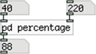
Figure 1-29. The “percentage” subpatch
This specific subpatch is quite simple, but we have already enclosed two objects in one. The more complex a function within a patch becomes, the more space we save by placing it in a subpatch, and the more readable our patch is, since we can give a name to the subpatch that corresponds to its function. This way we can even avoid writing comments, as our patch is self-explanatory.
Abstractions are somewhat different than subpatches. They are also Pd patches used as objects, but instead of creating them inside a parent patch (and saving them only through their parent patch), we create them independently of any other patch. Abstractions are essentially pieces of code that we very often use, so instead of making that specific piece of code over and over again, we create it once, and use it as is. Take a simple example—a hertz-to-milliseconds converter. This is a very simple patch to create; it is shown in Figure 1-30.

Figure 1-30. Contents of the “Hz2ms” abstraction
In this patch, we provide a value to [swap 1000]. What [swap 1000] does is get a value in its left inlet and output it out its right inlet, and output 1000 out its left inlet; in three words: swaps its values. Check its help patch for more information.
Pd’s objects will receive either hertz or milliseconds as time units, so it’s very helpful to have an object that converts from one to the other. But Pd doesn’t have such an object, and creating this patch (no matter how simple it is) every time you need to make this conversion would be rather painful. What you can do is create this patch once and save it to a place where Pd will look at. This is done in a few ways. One way is to save your abstraction in the same folder with the patch where you’ll use that abstraction. This way, the abstraction will be more project -specific rather than generic. The one in Figure 1-30 is a very generic one. What we’ll do is create a folder called abstractions, inside the pd_patches folder, and set that folder to Pd’s search path. To do this, go to Edit ![]() Preferences (on OS X, go to Pd-extended
Preferences (on OS X, go to Pd-extended ![]() Preferences). You’ll get a window where you can set a search path for Pd. This is shown in Figure 1-31.
Preferences). You’ll get a window where you can set a search path for Pd. This is shown in Figure 1-31.

Figure 1-31. Pd’s Preferences window
Click New... and a dialog window will open. Navigate to the newly created abstractions folder and click Choose. In Pd’s Preferences, click Apply. You won’t see anything happening, but the search path has been stored. Then click OK and the window will close. Now save the patch to the abstractions folder with the name Hz2ms, which stands for “hertz to milliseconds.”
For Pd to be able to use the newly set search path, you must quit it and restart it. Once you restart Pd, open a new window, put an object, and type Hz2ms. If all goes well, you’ll see an object with that name. If instead of an object you get a red dotted rectangle and a message in Pd’s console, like the one shown in Figure 1-32, check the search path in Pd’s Preferences, or make sure that you typed the name of the abstraction correctly.

Figure 1-32. An error message in Pd’s console
In a locked patch, clicking the abstraction opens the actual patch, like with subpatches. What is different from the subpatch is that the abstraction is ready to use whenever you launch Pd, and you don’t need to create it anew every time. Abstractions have more advantages, concerning arguments, name clashes, and others, but we’re not going into too much detail now.
Both the subpatch and the abstraction have their own purposes, and you can’t say that one is generally superior to the other. In different occasions, you might need to use one of the two. Also mind that both can be used in the signal domain by using [inlet~] and [outlet~]. Throughout this book, we’ll use both abstractions and subpatches.
Control Domain vs. Signal Domain
You’ve already learned that the signal domain runs for as long as the DSP is on, while the control domain will run only when it is told to (with a bang, for example). One thing you’ve also seen is a combination of the two. In the square wave oscillator patch that you made, you connected a number atom to the right inlet of [<~ ]. You also connected number atoms to [phasor~] to control its frequency, but that is not really affected by the difference between the two domains. Usually when you combine the two domains, you get annoying clicks when you give input from the control domain to the signal domain.
In the case of the square wave oscillator, these clicks are not really audible, because the square wave form is itself very “clicky.” Let’s take another example, one where you control the amplitude of a sine wave. Controlling the amplitude of a signal in digital electronics is simple multiplication with values between 0 and 1.
Since a digital signal is a stream of numbers, when you multiply these numbers by 0, you’ll get a constant 0 (remember the woofer’s positions; this would be silence). Multiplying the number stream by 1 will give you the number stream intact, hence the signal in its full amplitude. All the values in between will give corresponding results. Go ahead and build the simple patch, as shown in Figure 1-33.

Figure 1-33. Controlling the amplitude of an oscillator
You’re dividing the output of the Hslider by 127 to get a range from 0 to 1 (sliders have a default range from 0 to 127). Turn the DSP on and use the slider (in a locked patch). The more you move it to the right, the louder you’ll hear the sine wave. Pay close attention to these amplitude changes; the faster you move the slider, the more clicks you hear. This is due to the clash between the control and the signal domain. In detail, [*~ ] refreshes its values in every new DSP cycle (as all signal objects do), which is done in blocks of 64 samples (no need to really grasp this detail though).Therefore, if you change the slider values quickly, [*~ ] will make sudden jumps from the previous value to the current, which is heard as a click.
To remedy this, you must make the value changes smoother. There’s a very useful object in Pd for this: [line~]. [line~] takes two values: the destination output value and an amount of time in milliseconds. [line~] will make a linear ramp in the signal rate, from its current value to the destination value, and this ramp will last as many milliseconds as you provide with the second value. Change the patch in Figure 1-33 to the patch in Figure 1-34.

Figure 1-34. Using [line~] to avoid clicks
Lock your patch, turn the DSP on, and click the two messages alternately. You should hear the sound of the sine wave come in and go out without any clicks at all. This is because [line~] makes a ramp from 0 to 1 in 100 milliseconds, and the other way around. This ramp smooths the changes and gets rid of the annoying clicks.
But what if you want to have a variable amplitude? You can combine the slider in Figure 1-33 with [line~], as shown in Figure 1-35.

Figure 1-35. Combining the Hslider with [line~]
$1 in the message means the first value that comes in its inlet. Here we provide one value only, so $1 will take the value of the slider. 100 is still the amount of milliseconds for the ramp of [line~]. Now, no matter how quickly you move the slider, there are no clicks at all. This is the way to combine the two domains—something that happens very often in Pd.
Audio Input in Pd
Apart from sound generators, in Pd we can also use audio input, from a microphone for example. We can use that input in many different ways. We can store it, like we did with the oscillator wave forms, and play it back in various ways, we can write it in delay lines and use that to play a delayed copy in various ways, we can apply pitch shifting, and many more. For now, we’ll talk about how to receive that input, and we’re going to play it straight away from the speakers.
The object that receives input from the computer’s sound card is [adc~], which stands for analog-to-digital converter, which is the opposite of [dac~]. In a new window, put an object and type adc~. You’ll get an object with no inlets and two outlets. The two outlets are the two input channels on your computer’s sound card. But the default input in Pd is the built-in microphone, which has only one channel. So we can give an argument to [adc~], which is the channel we want to use; in this case, it’s 1. So click the object to make it editable, and type adc~ 1 (make sure that you put a space between the name of the object and its argument). Now the object has one outlet. Put a [dac~] and connect [adc~ 1] to both inlets of [dac~]. If you turn the DSP on and your speakers are quite high, you’ll get feedback, meaning that the audio that goes out the speakers will immediately go back in through the microphone, creating a loop, and it will most likely create a high and rather loud tone. To avoid that, you can use headphones for this patch. Now if you talk close to your computer’s built-in microphone, you’ll hear your voice through the headphones. Maybe the output is a bit delayed; that is because digital audio takes some time to make its calculations before it outputs sound. In the following sections, we’ll talk about a way to reduce that delay.
Basic Electronic Music Techniques
Now let’s cover some basic electronic music techniques with Pd. We’ve already created the four basic oscillators, but now we’re going to create some more interesting sounds by using them.
Additive Synthesis
The first technique we’re going to look at is called additive synthesis, because we use many oscillators (usually sine waves) added together to create more interesting timbres. Figure 1-36 shows an additive synthesis Pd patch.

Figure 1-36. Additive synthesis Pd patch
In additive synthesis, if we want to create a harmonic sound, we provide a base frequency, and we multiply it by the order of each oscillator. For the first oscillator, we multiply it by 1, for the second by 2, and so forth. Something else we do in the patch shown in Figure 1-36 is set the amplitude of each oscillator to the reciprocal of its order, so the first oscillator will have full amplitude, the second will have one half of its amplitude, the third will have one-third, and so forth. Note that multiplying requires less CPU than dividing, so instead of dividing, we multiply each oscillator’s output by the reciprocal of its order. Mind the multiplication at the bottom of the patch. When we output more than one signal as they are being added, therefore we must scale them to make sure that their sum won’t go over 1 or below –1. To achieve this, we multiply the total output by the reciprocal of the number of signals we send to the speakers; here it’s 1 ÷ 6 = 0.16666.
The more oscillators we use, the more it will sound like a triangle oscillator, because this is the algorithm the triangle wave form uses. Still, you need many sine wave oscillators to make them sound like a triangle. With additive synthesis, we can create more textures by providing frequencies to each oscillator that are not integer multiples of the base frequency. This will create non-harmonic sounds, but you might find very interesting textures this way.
Another aspect to experiment with is the amplitude of each oscillator. By changing these, the timbre of the sound changes drastically. Try some random values between 0 and 1 for each oscillator to hear the result. The way to create additive synthesis shown here is not the most effective one; usually, we prefer to use abstractions, as they reduce patching to a great extent. Still, it shows how additive synthesis works rather clearly. We’ll see how to utilize abstractions for additive synthesis in one of this book’s projects.
Using a lot of oscillators might give nice results, but it requires a lot of CPU, plus it can be cumbersome to create some textures. There are techniques that use only a few oscillators (two at least) and can give very interesting sounds. We’ll look into the most basic ones and we’ll start with the ring modulation (RM). This is a quite simple technique; it is the multiplication of two signals. We’ll use sine waves for all the techniques in this section, but you can experiment with any wave form we’ve already built. Make the patch shown in Figure 1-37.

Figure 1-37. A ring modulation patch
Lock your patch, turn the DSP on, and start dragging your mouse in the number atoms, or use sliders instead. (Although you might want to multiply their output to a range other than 127; multiply them by 3, for example.) You’ll start hearing two tones, which are the addition and the subtraction of the two provided frequencies. For example, if you type 300 in one number atom and 5 in the other, you’ll hear the frequencies 305 and 295. Sometimes the subtraction of the two frequencies result in a very low frequency (if, for example, you provide 305 and 300, you’ll get 605 and 5), which are not audible by the human ear. Keep on dragging your mouse upward till you start hearing two tones. Experiment a bit till you find some interesting results. You can also combine RM with the additive synthesis patch in Figure 1-36, where one of the two oscillators in Figure 1-37 will be replaced by the additive synthesis patch.
Amplitude Modulation
The next technique is the amplitude modulation (AM). It is very similar to the ring modulation. Again we multiply two signals, but we use one signal to modulate the amplitude of the other. As we’ve already seen, to modulate the amplitude of a signal, we need to multiply it with values between 0 and 1. But oscillators give values from –1 to 1. To bring one of the oscillators to the desired range, we need to apply some scaling and offset. First of all, we need to shrink the oscillator’s range to its half. We do this by multiplying it by 0.5 (remember that multiplication in computers require less CPU than division, so instead of dividing by 2, we prefer to multiply by 0.5). Multiplying by 0.5 will make the oscillator go from –0.5 to 0.5. If we add 0.5 (this is the offset), it will go from 0 to 1.
So, the patch in Figure 1-37 changes slightly and becomes the patch in the Figure 1-38.
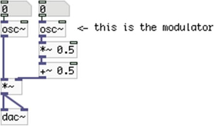
Figure 1-38. An amplitude modulation patch
Give a high enough frequency to the left oscillator (depending on your speakers; if you use laptop speakers, you should give at least 200) and a very low one (like 1) to the right oscillator, which is the modulator. You should hear the tone of the left oscillator come in and out smoothly. The higher you bring the modulator’s frequency, the faster these changes will happen. If you bring it too high (above 20), you’ll start getting similar results to the ring modulation. This is because humans can hear frequencies as low as 20 hertz. Using lower frequencies are not immediately audible, but they can effectively change the amplitude of another audio generator. In this case, the oscillator is called an LFO (low-frequency oscillator). If we provide a frequency higher than that, then it enters the audible range and we start hearing it immediately (and it’s no longer an LFO).
Next in line is the frequency modulation (FM). Here we use one oscillator, called the modulator, to modulate the frequency of another oscillator. The patch to do this is shown in Figure 1-39.

Figure 1-39. A Frequency modulation patch
Figure 1-39 includes some comments describing the role of each element. The carrier is the frequency of the oscillator that we actually hear, which is called the carrier oscillator. The modulator is the frequency of the oscillator that modulates the frequency of the carrier oscillator. The index is the amount of modulation the modulator will apply to the carrier. What actually happens is that the frequency of the carrier oscillator goes up and down, from the carrier frequency + the index, to carrier frequency – the index. If you think about it, an oscillator outputs values from –1 to 1. Whatever number we multiply this with will give us the multiplier and its negative. If, for example, we multiply the modulator by 2, it will go from –2 to 2; if we multiply it by 5, it will go from –5 to 5. This resulting output goes into the right inlet of [+~ ], where it is added to the carrier frequency, which is steady, and the output of [+~ ] goes into the frequency inlet of the carrier oscillator. The frequency of the modulator sets how fast these carrier frequency changes will happen. Figure 1-40 illustrates this.

Figure 1-40. FM illustration
If the horizontal axis of the graph is 1 second, the carrier frequency is 300, and the index is 50, the carrier oscillator’s frequency will go from 350 to 250 about three times a second (as many as the peaks in the graph) in a sine fashion. If the modulator frequency is quite low, what we hear is a vibrato-like sound (especially if we keep the index low as well). The higher the frequency of the modulator, the less we can tell that the frequency of the carrier oscillator is actually oscillating, and what we start to perceive is more tones around the carrier frequency. The higher the index, the broader the spectrum of the resulting sound becomes.
This technique is very common in electronic music, as you can create complex and interesting textures using only two oscillators. Experiment with all three values and try to find sounds that are interesting to you.
The last technique is the envelope, which we will use for amplitude. The previous four techniques dealt with timbres by using oscillators in various ways. One thing that none of these techniques included was some sort of amplitude evolution. Although AM did modulate the amplitude of an oscillator, that modulation had almost no variation, but a steady oscillating fading in and out. Some musicians tend to treat sound in a different way, where sounds evolve both in frequency and amplitude, with crescendo, decrescendo, and similar characteristics. An amplitude envelope is the evolution of the amplitude in time. By applying it to an oscillator (or to any of the preceding techniques), we can control its amplitude to a great extent, from simple to very complex ways.
Pd has vanilla objects that can create envelopes, but it can be rather cumbersome and not very intuitive, especially if someone is not very familiar with programming and Pd itself. For this reason, we’ll use an external object that is part of Pd-extended. This object is called envgen (for envelope generator) and it is part of the “ggee” library. A library is a set of external objects. It is very important to know which library each external that we use belongs to. To create this object, we need to specify its library, and that is done in a few ways. For now, we’ll use the simplest one, which is to type the name of the library first, then a forward slash, and then the name of the object. In this case, put an object in a new window and type ggee/envgen. Figure 1-41 shows what you should get by typing this.

Figure 1-41. The “envgen” external object from the “ggee” library
This object is actually a GUI, as you might have already guessed. It is designed to work with [line~], where it sends sequential lists to it. The envelope we’ll design is called the ADSR, which stands for Attack-Decay-Sustain-Release. It is the most common amplitude envelope that is used in many synthesizers, commercial or not. The ADSR is a simple imitation of the behavior of the sound of (plucked) acoustic instruments. The Attach part of it goes to full amplitude in a short time. The Decay part goes down to a lower amplitude, where it stays for a while, and this is the Sustain. Lastly, the Release goes down to zero amplitude in a short time. An ADSR envelope is shown in Figure 1-42.

Figure 1-42. An ADSR envelope with [ggee/envgen]
To create this, lock you patch and hover your mouse over the peak of the graph in [envgen], where you see a small circle. Drag this to the left a bit. To create more breakpoints (that’s what the points where the lines break are called), click anywhere inside the GUI. To move an existing point, click it and drag it, like you did with the first point. To delete a point, click it and hit Backspace.
The rising part of the envelope in Figure 1-42 is the Attack; the first falling part is the Decay; the horizontal line is the Sustain’ and the last falling part is the Release. Make the patch shown in Figure 1-43. The “duration 2000” message sets the duration of the envelope in milliseconds. The bang activates it. Turn the DSP on, lock your patch, click the “duration” message, and then click the bang message. You should hear the sine wave fade in and out in the fashion of the graph of the envelope, which should last two seconds in total. Go ahead and try different envelopes. Also try them in combination with the other techniques in this section.

Figure 1-43. An ADSR envelope in action
An envelope can be used in any control parameter of a sound, like the frequency, the index in FM, and so forth.
Figure 1-44 shows a patch where the modulator frequency, the index, and the amplitude of FM synthesis are being controlled by an [envgen] each. Mind the [trigger], where instead of f, we type b, which stands for “bang.” In this patch, [trigger] sends the bang it receives from left to right.

Figure 1-44. FM with envelopes controlling the modulator frequency, the index, and the amplitude
It is not very important to use here, but it’s good practice to get used to it. With the “duration” message on the other hand, it is even less important where it will go first, as this message causes no execution at all. As with the patch in Figure 1-43, lock your patch, click the “duration” message, turn on the DSP, and click the “bang” message. Experiment with different envelopes and durations.
Note that setting minimum and maximum values for [envgen] can be achieved with arguments. But for now, we don’t give any arguments and use the object as is, where it defaults to the range 0–1. Check the help patch to get more information about its use.
We have now covered five basic techniques of electronic music, which we will see later on as build musical interfaces. We’ve seen these techniques in their simplest form. In the following chapters, we will make more efficient, but also a bit more complex, use of them.
Delay Lines in Pd
A delay line is different than the delay mentioned earlier. A delay line delays sound intentionally. Actually, using delay in many music styles is a much celebrated effect, which has been around for a long time. Pd has built-in objects for that: [delwrite~], [delread~], and [vd~]. [delwrite~] is a bit like [tabwrite~]; it takes two arguments though. The first argument is the name of the delay line (like tables, delay lines need to have names so that we are able to access them), and the second is its length in milliseconds. In the previous patch with [adc~ 1] and [dac~], disconnect [adc~] from [dac~] and connect it to [delwrite~ my_delay 1000]. This is a delay line called “my_delay” and it will store 1 second of audio. Apart from its similarity with [tabwrite~], [delwrite~] will write on the delay line continuously, as long as the DSP is on. It doesn’t take a bang, and you can’t control the beginning and ending of writing to the delay line.
[delread~] will read audio from a delay line. It also takes two arguments: the first is the name of the delay line and the second the delay time in milliseconds. Put a [delread~ my_delay 500] in your patch and connect it to [dac~]. Figure 1-45 shows what your patch should look like. In this patch, [delwrite~] takes audio from the built-in microphone of your computer and writes 1 second to the delay line, called “my_delay”. When that second is over, it goes back to the beginning of the delay line and overwrites whatever was stored there; it does this for as long as the DSP is on. [delread~] reads from that delay line (because its first argument is the same with the first argument of [delwrite~]), but delays its reading by half a second, which is the second argument. If the second argument of [delread~] exceeds the second argument of its corresponding [delwrite~], the delay time is automatically clipped to the length of the delay line (in this case, 1000 milliseconds). If you turn on the DSP and talk into the microphone, you’ll hear your voice delayed by half a second.

Figure 1-45. Simple delay line patch
This might not be a very interesting use of delay, so let’s enhance it a bit. One feature of delay lines is feedback. What was not desired in the previous section, where we introduced [adc~], is desired when it comes to delay. If we send the audio read by [delread~] back to its corresponding [delwrite~], along with the audio that comes in from the built-in microphone, all audio stored in the delay line will be stored again, but delayed by 500 milliseconds. If we simply connect these two objects, we won’t have any control over it, and the delay line will keep on writing its own audio back to itself along with the audio that comes in through the computer’s microphone. To be able to control the feedback, we need to send the output of [delread~] to a [*~ ], which will control its level, and then to [delwrite~]. Figure 1-46 shows a feedback delay patch.

Figure 1-46. Feedback delay line patch
As I’ve already mentioned, the default range of Hslider is from 0 to 127. But multiplying the delayed sound by such a great number will greatly amplify it and distort it, which might not be so pleasant to your ears . What we did in a previous example with a slider was to divide its output by 127, so we get a range from 0 to 1. Another way to do that is to use its properties. Right-click it and select Properties. A window like the one shown in Figure 1-48 will show up. Go to the field named output-rage: and set the value in the right: field to 1. Click Apply and OK, or simply hit Return. This way, you can have any desired range. It might be advisable to place a comment next to a slider that has its range changed. When a slider is controlling the amplitude of a signal that’s coming out through the speakers, it’s rather obvious that its range is from 0 to 1. Mind that we send the output of the slider to the message [$1 20] and then to [line~]. This is to avoid clicks, as I mentioned in the “Control Domain vs. Signal Domain” section of this chapter. Turn on the DSP and start playing with the slider as you talk into the microphone.
[delread~] has one control inlet, which sets the delay time (it will override the second argument). Using it in real time will create clicks as we combine the control and the signal domain without using [line~] (it’s not possible to use [line~] here, as the inlet itself is a control inlet). If we want to be able to change the delay time on the fly, we must use another delay object: [vd~ ]. “vd” stands for variable delay. Change [delread~] in your patch with [vd~ my_delay]. [vd~ ] takes one argument only, which is the name of the delay line. You can’t set the delay time with an argument, but only with input in its inlet. Make your patch look like the one shown in Figure 1-47.

Figure 1-47. Delay patch using [vd~ ] instead of [delread~]

Figure 1-48. Slider’s properties window
Now you can play with both the feedback amount and the delay time. Again, if you’re not using headphones, be careful with the physical feedback that might occur. Mind that we’re using [line~] with [vd~ ] too, in order to avoid clicks.
Before closing this section, let’s make a final enhancement to our delay patch. Let’s use an oscillator to control the delay time of [vd~ ] to see how sound generators can act as controllers. Our patch remains more or less the same, only the input to [vd~ ] changes. Figure 1-49 shows this.

Figure 1-49. Using an oscillator to control the delay time of [vd~ ]
Since oscillators output values from –1 to 1, we apply scaling and offset to get values from 100 to 500 (think of simple math to understand how this is achieved). Give a very low frequency to [osc~], like 0.1 in order not to get changes in the delay time that are too fast. Turn on the DSP and play with. You’ll hear the delayed audio being repeated faster and faster, and then slower and slower. Also, the faster the repetitions get, the higher their pitch becomes, and vice versa. Try different oscillators with it to see how it sounds.
Reverb
Reverb is another celebrated effect in lots of music styles. It simulates the depth given to sound in large rooms. In Pd-extended, there is a vanilla abstraction for reverb called “rev3~”. Another option is the “freeverb~” external, which is also included in Pd-extended. A nice way to test both of these reverbs is to combine them with the audio file playback patch, shown in the “Using Tables in Pd” section in this chapter. Check their help patches to see how to use them, and place them (one at a time) between [tabplay~] and [dac~] (use the arguments of [rev3~] help patch before trying your own values). Better try a rather dry audio file to hear the full effect of the reverb. We won’t go into more detail about how to make the patch, as by now you should have gained some fluency in making simple patches.
Pd-extended has a variety of raw filters and a few user-friendly ones. The raw filers are [rpole~], [rzero~], [rzero_rev~], [cpole~], [czero~], [czero_rev~], and [biquad~]. These are quite tough to handle because they require quite some knowledge on filter theory. Just for the information, “rpole” stands for real pole, and “cpole” stands for complex pole. You don’t really need to worry about understanding all of this, as a few user-friendly filters are included as well. These are [lop~], [bp~], [hip~], and [vcf~], where “lop” stands for low pass, “bp” stands for band pass, “hip” stands for high pass, and “vcf” stands for voltage controlled filter.
[lop~] and [hip~] have one signal and one control inlet. The control inlet takes a frequency value (which can also be set as an argument), which is called the cutoff frequency. It is called “cutoff” because they will let all frequencies below or above that pass. The low pass will let the frequencies below the cutoff pass, and the high pass will let the frequencies above it, hence their names. The left inlet, which is the signal inlet, takes the signal to be filtered.
[bp~] and [vcf~] are somewhat different. They both have three inlets, the second of which receives the center frequency. It is called like that because they both let a band around that frequency pass (hence “band pass”). The right-most inlet takes the so-called Q, which is the width of the band of the frequencies that pass. Both of these values can be set as arguments in the case of [bp~]. [vcf~] takes one argument only, which is the Q. The difference between [bp~] and [vcf~] is that the latter can have its center frequency controlled by a signal (an oscillator for example); whereas [bp~] takes a signal only in its far-left inlet, which is the signal to be filtered, like with [lop~] and [hip~], and both the center frequency and the Q inlets are control inlets.
[biquad~] is not considered a raw filter, but it’s still difficult to handle. It takes a list of five parameters, and can more or less take the form of any kind of filter (low pass, shelving filters, and others). You need to know how to calculate the five coefficients to design the desired filter. Since it is not very user-friendly, we won’t be using it in this book.
An obvious way to use these filters is to filter out some high, low, or middle frequencies of a sound. Again, you can test them with a sound file, like you did with the reverb. Another way to use these filters is with oscillators to shape their wave forms. Figures 1-50 and 1-51 show a square wave and a triangle wave oscillator, respectively, passed through a low pass and a band pass filter, respectively. If you want to build these two patches, go to the properties of each array. Give each the appropriate name (“unfiltered” and “filtered”) and change their size to 512. Don’t have both patches open at the same time, as you will have each array twice, using the same name, and that will create a clash and warning messages in Pd’s console. [metro] is an object that outputs bangs in time intervals provided via its argument (or its right inlet) in milliseconds. Check the help patch for more information.
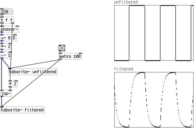
Figure 1-50. A square wave oscillator passed through a low pass filter
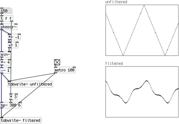
Figure 1-51. A triangle wave oscillator passed through a band pass filter
You can see how the shape of the oscillator changes drastically when filtered. This might be desirable for the immediate audio result, but also for using them as controllers in various techniques, like FM. Go back to the “Basic Electronic Music Techniques in Pd” section and try the patches shown there, with filtered oscillators. You’ll see that the variety of sounds you can create will expand greatly.
Before we close this section, let’s show [vcf~] in action and its advantage of being able to control its center frequency with signals. Build the patch shown in Figure 1-52. The [pd triangle~] subpatch contents are shown in Figure 1-53, although by now you should be able to tell without being shown.
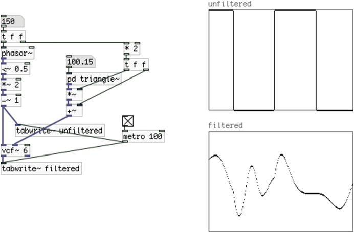
Figure 1-52. [vcf~] in action

Figure 1-53. Contents of [pd triangle~] from Figure 1-52
The result of this specific patch is definitely for hearing as well, and not only for graphing its output. What happens is that the center frequency of the filter is being controlled by a triangle oscillator. In Figure 1-52, the values output from the [pd triangle] subpatch, go from 0 to 600, in a triangle fashion. The frequency of the triangle is a little bit above two-thirds of the frequency of the filtered square wave oscillator. This small difference creates a slowly evolving shift in the timbre. Put a [dac~] in your patch and listen to the result. Try different values for both oscillators. As you can imagine, this is a kind of modulation, which could be included in the modulation patches in the “Basic Electronic Music Techniques in Pd” section.
We’ve covered most of the basics of Pd, so now we can talk about more generic things. Here we’ll talk about how to connect objects, messages, numbers, and so forth, wirelessly. Visual programming can be very intuitive, because of graphing the data flow in a program, but the more complex a patch becomes, the more difficult it is to read. Figure 1-54 shows a patch that’s pretty messy.

Figure 1-54. A rather messy patch
Thankfully, Pd provides a way to connect things without the connection cords, and this makes things a lot cleaner. In the control domain, we can connect things wirelessly using [send] and [receive], abbreviated [s ] and [r ]. These objects take one argument, which is the name to send to and to receive from. A [send my_send] will be heard by a [receive my_send], as shown in Figure 1-55.

Figure 1-55. A wireless connection
You can have as many [send]s and [receive]s with the same name as you want. Mind that whenever we use these objects, we’ll use their abbreviated aliases, [s ] and [r ].
In the signal domain, things are a bit different. There are the [send~] and [receive~] objects (also abbreviated [s~] and [r~]), but you can have only one [s~] with many [r~]s. If you want to send many signals to one destination (the [dac~] for example), you need to use the [throw~]/[catch~] pair, where you can have many [throw~]s with the same name, sending signals to one [catch~] with that name. Figures 1-56 and 1-57 show the [s~]/[r~] and [throw~]/[catch~] pairs, respectively.

Figure 1-56. A [s~]/[r~] pair

Figure 1-57. A [throw~]/[catch~] pair
As mentioned in the additive synthesis patch, signals sent to one destination are being added. You can see that in Figure 1-56, where the graph of the signals exceeds the limits of –1 and 1 (the frame of the graph). When using [throw~]/[catch~] pairs to send sound, make sure that you scale the sum of signals sent to [catch~] to keep them within limits. If the audio signal limits are exceeded, they will be clipped before they reach the sound card. So the graph shown in Figure 1-57 will actually look like the one in Figure 1-58, and the resulting sound will be distorted.

Figure 1-58. A clipped audio signal
Before we close this section, I’ll note that you must be careful when using wireless connections, as a patch can become difficult to read because the connections are not immediately visible. Wireless connections are there to facilitate us when a patch becomes too dense or when it is very difficult to use wired connections for other reasons. Most of the time, they are much less than the wired ones. A good balance between wired and wireless connections is an optimal goal. But ultimately, this depends on the programming style of each person.
Another thing to note is that when using one [send] with many [receive]s in the control domain, there is no way to force the execution order, as the order the [receive]s were created doesn’t have the same effect as the order of the connections we make (data will go to the first connection made, but not necessarily to the first [receive] created). Be very careful when using this pair this way. There is an external object that remedies this situation, [iemguts/oreceive] (iemguts is the name of the library that the external belongs to).
Until now, we have used the default settings for audio, but we haven’t dealt with MIDI at all. The audio settings let you configure various settings, like the sample rate, the delay (not the same thing as the delay we saw previously), and the block size. They also let you choose an external sound card and set the number of channels both for input and output. In general, when you make music with a computer, it is advisable to have an external sound card. This is for better performance, for more noise-free audio, for having more than two channels for input and output, and so forth. A discussion on sound cards is beyond the scope of this book, so I’ll presume you already have a sound card and take it from there. If you don’t have one, it’s not really a problem, but read this section because it is helpful for other things concerning your audio settings.
To change the audio settings in Pd, go to Media ![]() Audio Settings.... The Audio Settings window will open. There are a few things you can change in this window. The first one is the “Sample rate,” which defaults to 44100. We’ll leave that as is for now, but if you want to play back audio files that have been recorded in a different sample rate, then you should set that rate here. The next field is the Delay, which defaults to 20 milliseconds in OS X and Linux, and to 100 on Windows. This is a delay set to give time to the computer to do its audio calculations. If you have too much latency with your audio input (for example, the patch with [adc~ 1]), try a smaller number. You should probably set the smallest number that doesn’t distort the sound.
Audio Settings.... The Audio Settings window will open. There are a few things you can change in this window. The first one is the “Sample rate,” which defaults to 44100. We’ll leave that as is for now, but if you want to play back audio files that have been recorded in a different sample rate, then you should set that rate here. The next field is the Delay, which defaults to 20 milliseconds in OS X and Linux, and to 100 on Windows. This is a delay set to give time to the computer to do its audio calculations. If you have too much latency with your audio input (for example, the patch with [adc~ 1]), try a smaller number. You should probably set the smallest number that doesn’t distort the sound.
To test your latency, go to Help ![]() Pd Help Browser and a window will open. In that window, go to Pure Data
Pd Help Browser and a window will open. In that window, go to Pure Data ![]() 7.stuff
7.stuff ![]() tools, and double-click latency.pd. A patch will open with instructions on how to use it. This patch calculates the latency created by Pd and reports interruptions and errors (if your system doesn’t have enough time to do its calculations). The next field is Block size, which defaults to 64. This is the number of samples in each block that the signal objects receive and output. We won’t really need a different block size in this book. Note, though, that the smaller the block size, the faster the audio, but the higher the CPU. We’ll also leave the Use callbacks tick box unticked.
tools, and double-click latency.pd. A patch will open with instructions on how to use it. This patch calculates the latency created by Pd and reports interruptions and errors (if your system doesn’t have enough time to do its calculations). The next field is Block size, which defaults to 64. This is the number of samples in each block that the signal objects receive and output. We won’t really need a different block size in this book. Note, though, that the smaller the block size, the faster the audio, but the higher the CPU. We’ll also leave the Use callbacks tick box unticked.
All this leads us to the Input device 1: field. If you have no sound card plugged in your computer, Pd will choose the built-in microphone, as shown in Figure 1-59. If you plug in a sound card, you’ll need to restart Pd, as it’s not going to see the sound card if it is already launched. If your sound card is not chosen by Pd automatically, click the (0)Built-in Microph menu and a pop-up menu will appear, where you can choose your sound card (make sure you have the necessary drivers for your sound card, if there are any. You must install them and make any configurations necessary before trying to use it with Pd).

Figure 1-59. The Audio Settings window in Pd
The field below Input device 1: is the Output device 1:, which sets the output sound card. You can have one sound card for input and another for output, if, for example, you want to use the built-in microphone and use your external sound card’s output.
The Channels fields set the number of channels for the input and the output. If you want to set up a quadraphonic system, this is where you’ll set the number of channels. In all the projects of this book, we’ll use a stereo setup, so we’re not going to change these fields. When you make the setting you want, click Apply and then OK. It will take a few seconds, and the Audio Settings window will close. Your settings are now ready and you can use your sound card with Pd.
To set your MIDI devices, go to Media ![]() MIDI Settings... and the MIDI Settings window will open, as shown in Figure 1-60.
MIDI Settings... and the MIDI Settings window will open, as shown in Figure 1-60.

Figure 1-60. The MIDI Settings window in Pd
As with the audio settings, you need to plug in your MIDI devices before you launch Pd, otherwise it won’t be able to see them. In the MIDI Settings window, you can choose your input and output devices. We’ll barely use any MIDI, only in Chapter 5, where we’ll build a MIDI keyboard synthesizer, but we’re covering this part in this chapter since you’re getting introduced to Pd. Usually, we use only input devices, like MIDI controllers, keyboards, and so forth, but you might also want to control a MIDI device from Pd (actually, Pd’s predecessor, Max, was initially made—by Miller Puckette as well— to control a hardware MIDI synthesizer).
In the MIDI Settings window, again you have two fields, Input device 1: and Output device 1:, like in the Audio Settings. This is where you choose your device. If you have more than one device, first click the Use multiple devices button and you’ll be able to choose more than one device both for input and output. When you select your devices, click Apply and then OK for your settings to be activated.
MIDI Settings on Linux
Setting your MIDI devices on Linux is a bit different. Launch Pd from the terminal with the -alsamidi flag, like this:
/usr/bin/pd-extended -alsamidi &
Open Pd’s MIDI Settings from Media ![]() MIDI Settings... and make sure there is at least one port for the input. If you’re using more than one MIDI device, you should set the number of ports appropriately. Click Apply and OK. Then in a new patch, put [notein] if you’re using a MIDI keyboard, or [ctlin] if you’re using a controller with potentiometers. Open its help patch and see if you get input from your device. If you don’t get input, go back to the terminal and type:
MIDI Settings... and make sure there is at least one port for the input. If you’re using more than one MIDI device, you should set the number of ports appropriately. Click Apply and OK. Then in a new patch, put [notein] if you’re using a MIDI keyboard, or [ctlin] if you’re using a controller with potentiometers. Open its help patch and see if you get input from your device. If you don’t get input, go back to the terminal and type:
aconnect -lio
This will print the available MIDI devices and software currently plugged in and running on your computer. In my computer I got the following:
client0:’System’[type=kernel]
   0’Timer          ’
   1’Announce       ’
client14:’MidiThrough’[type=kernel]
   0’MidiThroughPort-0’
   ConnectingTo:128:0
    Connected From: 128:1
client 20: ’nanoKEY’ [type=kernel]
    0 ’nanoKEY MIDI 1  ’
    Connecting To: 128:0
    Connected From: 128:1
client 128: ’Pure Data’ [type=user]
    0 ’Pure Data Midi-In 1’
    Connected From: 14:0, 20:0
    1 ’Pure Data Midi-Out 1’
    Connecting To: 14:0, 20:0
What I get is that I have a Korg nanoKEY sending to port 0, and Pd receiving in port 0 (it sends to port 1). The following example connects the nanoKEY to Pd:
aconnect nanoKEY:0 ’Pure Data’:0
Pd’s name is two words, so you need to place it without quotes.
A Bit More on MIDI
Since we’re talking about MIDI, let’s talk a bit about how to receive input from various MIDI devices. Data from MIDI keyboards can be fetched with [notein]. If you provide no argument to it, it will have three outlets and no inlets. The outlets from left to right are the MIDI note number, the velocity, and the MIDI channel number. If you know the channel, you can set it via an argument, and [notein] will have only two outlets, for the first two. We’ll see this object in more detail in Chapter 5.
Controllers with sliders and potentiometers send Control Change messages, which can be retrieved with [ctlin], which stands for control in. Open its help patch and use your already set controller to see the input it gives. Again this object has three outlets and no inlets, and the outlets give the controller value, the controller number, and the channel number. The last two can be set via arguments. Check the help patch for more information. Also, click the [pd Related_objects] subpatch to see all the MIDI objects available in Pd.
Additional Thoughts
Before we move on to the next chapter, I’d like to give a few tips concerning Pd programming. First of all, make sure that you save your patches in an organized way. Some people prefer to save files depending on the project; others prefer to have a tree structure of the files in a single program or programming environment. You might prefer a different way. The more you deal with Pd, the more files you’ll save on your computer. Whether you are a hobbyist or you want to make things with Pd professionally, it’s best that you find a way to organize your patches that suits you well.
Make sure that your patches are clean. Placing objects here and there will most likely create a chaotic patch. Try to have your objects aligned as much as you can. Make use of subpatches, and whenever applicable, abstractions. Try to make your patches self-explanatory (by giving describing names to subpatches, for example), and wherever this is not possible, use comments to describe what happens in that specific part of the patch. Even if you know what each object does in a patch, if there are not enough comments (or no comments at all), it might still be very difficult to understand what happened. This applies to your own patches too; when you come back to them after some time (even a couple of weeks can be enough, to make things confusing).
Use [trigger] whenever necessary. This means that wherever one piece of data goes to more than one destination, and the order matters, always use [trigger]. Not using it will very likely create bugs that are very hard to trace. Also, it makes the understanding of a patch very difficult, or even impossible. We haven’t seen all features of this object yet, as apart from forcing the order of execution, it also converts data types (it can convert a float to a bang, for example), so in the chapters that follow, you’ll see that it is a very important and helpful object.
Try to build simple things and to make them more complicated as you go. Trying to create something complex and beyond your skills will cause confusion and disappointment. With programming, you can create amazing things, but it takes time to handle a programming language. Take one step at a time, and try to take joy even with very simple programs that you build. As already mentioned, learning Pd is a matter of personal practice, and if you practice it frequently, you’ll find yourself building rather complex programs before you expected.
I should mention that at the time of writing (August 2015), Pd-extended is not being maintained. Pd-vanilla, on the other hand, is being actively maintained by Miller Puckette, with new features added and new versions released frequently.
Pd’s community is very active too, with lots of developers running and sharing their own projects. There has been a discussion among the community as to what route should be taken to either revive or replace Pd-extended. The prevailing idea for now seems to be one that centralizes external objects in a repository that you can pull from and add to your Pd-vanilla. Since Pd is open source, this kind of issue is likely to arise sometimes. But with an active community like the one around Pd, there’s no fear that all issues will be solved. Still, the current version of Pd-extended is fully functional and can be used at both an amateur and a professional level. If you keep using Pd, it’ good to stay up-to-date as to how it is going to be maintained in the future. You can place yourself on Pd’s mailing list, which you can find on its web site, or you can sign up on the Pd forum at http://forum.pdpatchrepo.info/.
Conclusion
This concludes the first chapter and the introduction to Pd, a very flexible and powerful programming environment. In this chapter, you have been introduced to Pd, its philosophy, some of its features, capabilities, but also to some basic techniques of electronic music in general. Learning how to use Pd is a matter of personal practice, though.
Later on in this book, we’re going to build more complex patches to make musical programs. What this book will try to provide is basic knowledge on the tools used, but also ways to research when you want to realize a personal project. The musical projects built here are limited, so they cannot meet every musician’s needs. What they can do is give inspiration and insight to musicians so that they can realize original projects of their own. The main focus in this book is to combine the physical world with that of the computer to make musical interfaces. The basics of this communication will be covered to such an extent, that you will be able to use these tools in many different ways, much more than the ones shown here.
Next are the Arduino basics, where you will be introduced to its language and some simple circuits, and to the communication features between Arduino and Pd.
______________________
1In contradiction to many programming languages, Pd has 0 when no argument is provided, instead of NULL.