
![]()
Getting Started with Musical Applications
You have now been introduced to all the necessary tools, so we can start building some real interfaces. In this chapter, we’re going to build a couple of rather simple interfaces on a breadboard. Since they’re not going to be finished projects, we’re not going to deal with soldering circuits on a perforated board, as the breadboard will serve just fine for our purposes. This chapter acts more like an introduction to using Pd and Arduino to create musical interfaces, and as a kickoff to making really interesting projects for your musical creations.
We’re going to combine things learned in the first two chapters (we’re not going to use any embedded computers or wireless communication) in a way that will create some more interesting sounds than the ones we’ve already made. We’re going to build two interfaces—a phase modulation interface and a simple drum machine, and we’re also going to combine them. The interfaces here will be fairly simple, but they cover the basis of a general approach to building finished projects.
Parts List
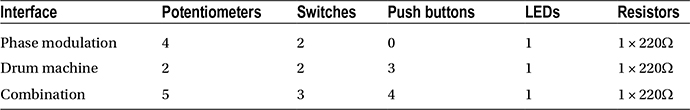
Table 4-1 lists the parts needed for each of the three interfaces. The third one is a combination of the first two, but it’s listed here as well.
Table 4-1. Parts List for the Interfaces of this Chapter
Phase Modulation Interface
The first project we’ll realize is a phase modulation Pd patch, controlled by some potentiometers and some switches with the Arduino. Phase modulation is a technique similar to frequency modulation, but slightly different. I didn’t cover it in the first chapter, but since we’ve already covered frequency modulation, it won’t be very difficult to understand what’s happening. It is a celebrated technique that can produce very interesting sound results with just a few elements. As in frequency modulation, in phase modulation there’s a carrier oscillator that has its phase (instead of its frequency) modulated by another oscillator. Again, there are three elements: the carrier oscillator, the modulator oscillator, and the index. To understand what is meant by phase, let’s think of a sine wave oscillator. Figure 4-1 illustrates how the waveform of a sine wave occurs.
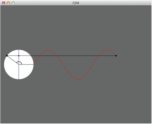
Figure 4-1. Sinusoidal waveform produced by a rotating angle
How Phase Modulation Works
The angle in Figure 4-1 (which is made in Pd, by the way) is rotating counter-clockwise, constantly. As it rotates, a straight line is drawn from the point where the rotating angle meets the circle circumference (if the sine wave has full amplitude) to the vertical axis of the circle. The end of the line that meets the vertical axis of the circle (indicated by a dot) is the sine of the angle. On the right side of the circle, the sine is translated in time, forming its waveform. When we modulate the phase of a sine wave oscillator, we’re actually modulating the rotation of the angle. So, instead of going constantly counter-clockwise in a steady frequency, it will change both direction and frequency according to the wave form of the modulator oscillator. When these changes occur slowly, we hear a glissando that goes up and down, around the carrier frequency. When these changes occur fast, what we perceive is a tone rich in harmonics. You can see that this effect is very similar to frequency modulation. You can get similar results with the two techniques, if the right coefficients are provided. It might be a bit easier to use phase modulation to control timber richness (at least to my experience); whereas with frequency modulation, you can control frequency shifts easier.
Making the Pd Patch
Since I’ve started by explaining the technique, we’ll use for the sound. Let’s first look at the Pd patch for this project. Figure 4-2 illustrates the patch, which I’ll explain in detail.
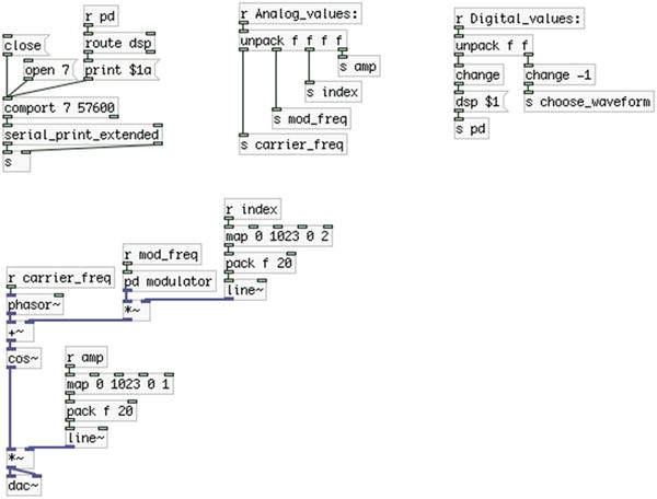
Figure 4-2. Phase modulation Pd patch
Receiving Values from the Arduino
On the top-left part of the patch we have [comport] with the serial port and baud rate arguments (the serial port argument is very likely to be different in your computer), along with some messages, which we’ll look at in a while. On the top-right part of the patch, we have the [r Analog_values:] and [r Digital_values:] objects that receive the corresponding values from the Arduino, exactly like in the help patch of the [serial_print_extended] abstraction. This time we’re using four analog values (four potentiometers) and two digital (two switches), which you’ll see when I explain the Arduino code and circuit.
Implementing Phase Modulation in Pd
On the lower part of the patch, we have all the signal objects, which is where the phase modulation is happening. On the left side, you see a [phasor~] connected to a [+~ ] and then to a [cos~]. Connecting a [phasor~] straight to a [cos~] will produce a pure cosine oscillator. [cos~] takes a signal in its inlet and multiplies that by 2pi. Sending a [phasor~] to it, which is a rising ramp from 0 to 1, creates a rising ramp from 0 to 2pi. [cos~] will give the cosine of this, which results in a sinusoid oscillator. This makes the name of [phasor~] meaningful, as it is actually the phase of the oscillator. If we place a [+~ ] between [phasor~] and [cos~] and connect another oscillator to the right inlet of [+~ ], we are modulating the phase of [cos~].
Building the Modulator Oscillator
On the right side of [phasor~], there is a subpatch called modulator. Figure 4-3 shows its contents. Here we can choose between the two waveforms for the modulator oscillator, which are a sinusoid and a triangle oscillator. Both oscillators are controlled by the same [phasor~], so they will have exactly the same phase. Again, we’re making the sinusoid by connecting [phasor~] to [cos~], instead of using [osc~], so we can share the phase between the two oscillators. On the right side we’re creating a triangle oscillator the same way we did in Chapter 1. On the top-right side of the modulator subpatch, you see a [r choose_waveform], which takes a value from [s choose_waveform] in Figure 4-2, which comes from the second switch of the circuit. Since a switch is controlling this value, it will be either a 1 or a 0. The triangle oscillator is controlled straight by that value. So whenever the switch is in the OFF position, it will output a 0, so the triangle oscillator will be multiplied by 0, and it will give 0 output. When the switch is in the ON position, it will output a 1, and the triangle oscillator will be multiplied by it, so it will output its waveform intact. The value of the switch is also sent to the cosine oscillator, but it first connects to [== 0] and then to the signal multiplication object. [== 0] takes in a value and tests if that value is equal to 0. If it is, the test is true, so the object will output a 1. If it’s not equal to 0, the test will be false, and the object will output a 0. So if we send a 0 to [== 0], it will output a 1, and if we send it a 1, it will output a 0. This is a very easy way to invert 1s and 0s. So, when the switch is in the OFF position, it will output a 0, and [cos~] will be multiplied by 1, therefore it will output its signal intact. When the switch is in the ON position, it will output a 1, and [cos~] will be multiplied by 0, producing 0 output. This way, we can easily use one ON/OFF switch to choose between two elements.
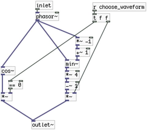
Figure 4-3. Contents of the modulator subpatch
Mapping the Index Values
On the right side of the modulator subpatch, you see a [r index] (in Figure 4-2), which takes its value from [s index], which comes from the third potentiometer of our circuit. [r index] is the connected to [map 0 1023 0 2]. This is an abstraction I’ve made that makes it very easy to map a range of values to another range. You can get it from my GitHub page at https://github.com/alexdrymonitis/miscellaneous_abstractions. This page contains various abstractions along with help patches, so it might be quite useful to you. Once unzipped, place all its contents to your “abstractions” folder, which is included in your Pd’s search patch. [map] takes four arguments, the lowest value of the original range, the highest value of the original range, the lowest value of the desired range, and the highest value of the desired range. In this case, we’re receiving an analog value from the Arduino, which has a 10-bit range.
This means that it will go from 0 to 2 to the 10th power minus 1, so from 0 to 1023. What we want is to get a range from 0 to 2, so the arguments we provide to [map] are 0, 1023, 0, 2. You can build a patch that does the same thing simply by dividing the input range by its highest value, and multiplying the result by the maximum desired value. In this case one would have to divide by 1023 (which is the maximum value of the analog pins of the Arduino) and multiply by 2. A division is more expensive as far as the CPU is concerned, and [map] avoids doing it. Open the abstraction if you want to see how it works. [map] then connects to [pack f 20]’s left (hot) inlet. [pack f 20] will pack the value coming in its left inlet along with the value 20, so it will output a list of these two values, which is sent to [line~]. To refresh your memory, [line~] takes a list of the target value and the ramp time in milliseconds, and it will make a ramp from its current value to the target value, which will last as long as the milliseconds provided by the second value of that list. It is used to combine the control domain with the signal domain, avoiding possible clicks that occur by this combination.
The output of [line~] goes to the right inlet of the signal multiplication object the modulator subpatch connects to. This way the value received by [r index] becomes the index of the phase modulation in our patch.1
At the bottom of the patch, we’re multiplying the output of [cos~], which is the modulated oscillator, and what we actually hear, by the values received in [r amp], which comes from the fourth potentiometer. We’re mapping that value to a range from 0 to 1, because that’s the range used to control the signal amplitude sent to the speaker. Again, we’re using [line~] to smooth out the value changes and avoid clicks, and we finally send that output to [dac~].
Handling the Values Received from the Arduino
Before we go on to the Arduino code, I must talk about the top-right part of the patch in Figure 4-2. [r Analog_values:] sends a list of four values (as many as the potentiometers we’re using), which is unpacked by [unpack f f f f] and each value is sent to its destination by the corresponding [send] object. That is pretty straightforward. The digital values get a different kind of treatment to be used properly. [r Digital_values:] receives a list of two values (as many as the switches we’re using) and unpacks it with [unpack f f]. Below [unpack], you see two [change] objects, where the right one has an argument, –1. [change] takes in a value and compares it to its argument (if no argument is provided, it compares it to 0). If the value is the same as the argument, [change] won’t output it. If it is different, it will output it and it will also update its arguments with the value it has just output. When we send the values of a switch to [change], we’ll get the switch value only when it becomes 1 (when the switch goes to the ON position), and [change] will update its internal value to 1. As long as the switch remains in the ON position, [change] won’t output anything, because its internal value is now 1, and the switch keeps on sending the value 1. When we put the switch to the OFF position, it will output a 0, and [change] will output it, since it’s different than 1, and it will again update its internal value. This way we can receive digital values only when they change, which is really necessary in some cases.
The left [change] is connected to the message “dsp $1”. “$1” will take the first value of an incoming list. Our list consists of one value only, so “$1” will take the value of the switch, when it goes through [change]. The message that will be constructed (“dsp 1” or “dsp 0”, according to the position of the switch) is sent to [s pd]. We can send certain messages to Pd, which can control certain aspects. The “dsp” message controls the DSP, as you can imagine. So sending a “dsp 1” message will turn the DSP on, and sending a “dsp 0” message will turn the DSP off. This way we can control the DSP from the Arduino, without needing to our computer’s keyboard or mouse.
The right [change] has an argument that is –1. This is there only to initialize this [change]. We do this because when we open the serial port, the data from the Arduino will start coming in, and if the corresponding switch is in its OFF position, it will send a 0. If we don’t provide an argument to [change], it will compare its incoming value to 0, and if the incoming value is 0, it won’t output it. We’re using this switch to control the waveform of the modulator oscillator, where sending a 0 will give a sinusoid, and sending a 1 will give a triangle. If [change] has no arguments and the switch is in the OFF position, nothing will come out of [change], so no oscillator will be chosen. By giving –1 as an argument to [change], we make sure that any position of the switch will go through as soon as we open the serial port (whether OFF or ON, 0 or 1), and we’ll immediately choose our modulator oscillator.
Sending Data from Pd to the Arduino
The last thing that I need to explain about this patch is the “print $1a” message in the top-right part of it. As we can send messages to Pd using [s pd], we can also receive messages from Pd, using [r pd]. In our case we connect [r pd] to [route dsp], so we filter out all messages sent by Pd, and receive only messages about the DSP. These will be either 1 or 0, according to the DSP state. So when the DSP is on, [route dsp] will output a 1, and when it’s off, [route dsp] will output a 0. We send that value to the “print $1a” message, which goes to [comport]. The word “print” will convert the rest of the message to its ASCII values (this is a feature of [comport]). Using “a” is a convenient way to diffuse the data we send from Pd to Arduino, as you’ve already seen in Chapter 2. This message receives the DSP state and controls an LED in the Arduino circuit, which indicates whether the DSP is on or off. This will be really necessary when we’ll be building interfaces with embedded computers, or when we’ll be using a wireless connection between the Arduino and Pd. In general, we need some kind of visual feedback for the state of the DSP, whenever we won’t have visual contact with the screen of the computer.
Arduino Code for Phase Modulation Patch
Now let’s take a look at the Arduino sketch. This is shown in Listing 4-1.
This is a modified version of the serial_print.ino sketch that comes with the [serial_print_extended] Pd abstraction. Some things are the same, but there are some new things as well, which I am going to explain.
Defining Constants, Variables, and Pin Modes
Lines 2 and 4 set the number of analog and digital input pins we’re using. We’re using four potentiometers and two switches. Line 6 sets the number of digital output pins we’re using, which is 1. This variable doesn’t need to be a constant, as it doesn’t define the size of an array, it will only be used in the test field of a for loop. In line 15 we run a for loop to set the pins where the switches are attached to as inputs with the pull-up resistors enabled. Notice that we add 2 to the i variable, because we use digital pins from 2 onward, as pins 0 and 1 are used for the serial communication between the Arduino and Pd. In line 19, we run another for loop to set the pin of the LED as output. Here we add the num_of_digital_inputs plus 2 to the i variable, because the variable starts counting from 0, but the pin we’ve attached the LED to is number 4.
Handling Input from the Serial Line
In lines 26 to 40, you see the same technique we used in the last sketch of Chapter 2. This is a technique that makes it easy to receive different kinds of information and diffuse it accordingly in the Arduino code. Line 27 defines a static int variable that will hold its value even after the function it belongs to has ended. Line 28 defines a variable that will hold the number of the pin we want to control, and line 29 stores the incoming bytes in a byte variable, one by one. Line 31 checks if the current byte is a numeric value, and if it is, it assembles all numeric bytes the original value sent. Here we’ll be sending only 0s and 1s, so temp_val * 10 could have been omitted, but if we want to send values with more than one digit, we’ll need that line exactly as it is, so we’re using it this way here as well. Line 34 checks if the current byte is an alphabetic character, and it if is, it stores that value to the which_pin variable. In line 35, we subtract ’a’ from in_byte, and in line 36 we add num_of_digital_inputs + 2 to that, so we can obtain the first digital output with the letter a, the second digital output with the letter b, and so forth. If in_byte is ’a’, then in_byte - ’a’ is 0. Adding num_of_digital_inputs + 2 makes it 4, which is the digital pin we’ve attached our LED to. Here, we’re using only one digital output, but if we used more, we could use incrementing letters of the Latin alphabet this way, to map each value to the corresponding pin.
Line 37 writes the value stored in temp_val to the which_pin pin using the digitalWrite function. This function is called only when we receive input in the serial line, and only if that input is an alphabetic character. This way we can save some processing power, since we’re not calling this function over and over again in each iteration of the loop function. After we call digitalWrite, we set temp_val to 0, so when we send a new value, it will be assembled anew.
Reading the Analog and Digital Pins and Writing the Values to the Serial Line
Lines 43 and 45 read and store the values read from the analog and digital pins respectively. In line 45 we use the exclamation mark to invert the readings of the digital pins because of the pull-up resistors, as if we didn’t use it, when a switch would be off, we would read 1 instead of 0. Lines 48 to 53 and 55 to 60, write these values to the serial line, using the print and println functions, so we can retrieve these values with the [serial_print] abstraction in Pd.
Circuit for Arduino Code
Now that we’ve gone through the Arduino sketch too, let’s see the circuit for this project. Figure 4-4 illustrates it.
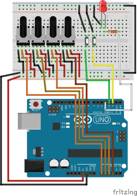
Figure 4-4. Phase modulation project circuit
The potentiometers must use analog pins 0 and onward, and the switches must use the digital pins 2 and onward for the Arduino sketch to work properly. The LED must be attached to the first digital pin after the switches. We’re not using resistors with the switches because we use the internal pull-up resistors of the Arduino processor, by using INPUT_PULLUP in the pinMode function. These resistors are different than the ones we need for LEDs, so we have to use a 220Ω external resistor with it. Notice that we use a jumper wire to connect the ground buses on bottom and top of the breadboard. This is because of the limited space on our breadboard. We’ve placed the LED on the upper part of the breadboard, and connected its ground pin to the upper ground bus. If we don’t provide ground from the Arduino, the bus won’t be grounded and the LED won’t work. Since we connect Arduino’s ground to the lower bus of the breadboard, we must connect the two buses with a jumper wire, so that the LED gets the ground too.
Once you’ve built the circuit, upload the sketch to your Arduino board, and open the Pd patch. Open the Arduino’s port in [comport] (making sure you use the correct baud rate, here 57600) and put the first switch to the ON position. You should see the DSP indication in Pd’s console turning green and being ticked, and the LED on your circuit lighting up. We could have controlled the LED straight from the Arduino code, without having Pd interfering. Controlling it from Pd, gives us more valid information about the DSP. If for any reason, we turn the DSP switch on, but the DSP doesn’t really go on, the LED won’t light up, so we’ll know that the DSP is not running. If we were controlling the LED only inside the Arduino code, we could face a situation where the DSP switch could be on, the LED as well, but the DSP not running, and we wouldn’t have an indication for it. Now we have eye contact with the computer screen, but in the case of an embedded computer, or a distant wireless connection, the LED would be our only indication for the DSP. For this reason, it’s very important to use LEDs controlled by Pd when building such interfaces.
Now you can use the fourth potentiometer to control the overall amplitude of the Pd patch, and the first to third potentiometers to control the carrier frequency, the modulator frequency, and the index, respectively. This is a quite simple interface, but it is nevertheless a completed one. We’ve built it to start getting the hang of such processes. The projects that are yet to come will realize even more musical ideas. Congratulations, you’ve built your first audio interface!
A Simple Drum Machine Interface
For the second interface, we’ll build is a simple drum machine. This is a bit more complex than the previous interface. Again, we’ll start with the Pd patch, which is shown in Figure 4-5.
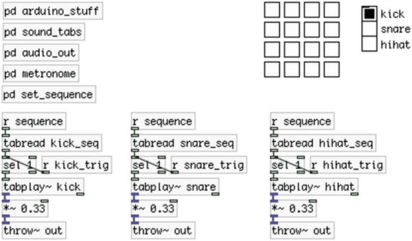
Figure 4-5. Simple drum machine patch
Building the Pd Patch
We’re going to use drum sound samples, instead of procedural audio (drum sounds generated by oscillators). You can register at freesound.org to get loads of audio samples that you can use for free. Mind the license of each sample, depending on what you want to do with it. You can use some of the samples even for professional reasons and earn money, but not all of them. Read about the different licenses (they’re three in total) if you want to do something else than personal use. Here we’re just building a simple drum machine for fun, so all licenses allow such use.
The Parent Patch
Part of the whole interface is in the parent patch, and part of it is in subpatches. This helps to keep things clear. In the parent patch, you can see a matrix of toggles, a Vradio, the [tabread] objects that read the sequence for each drum sound, and the [tabplay~] objects that play the stored audio files. Since we have three sounds in total, we’re multiplying their output by 0.33, so that their sum doesn’t exceed 1, in case they are all triggered together.
Notice that the toggles don’t have inlets or outlets. This is because we’ve set some things in their properties, which you’ll see a bit further on. The same applies to the outlet of the Vradio. Once you’ve built the lower part of the patch, let’s build the subpatches, one by one.
Figure 4-6 illustrates the contents of the arduino_stuff subpatch. This is where we have [comport] listening to the Arduino serial port, at a 57600 baud rate. Below it, we have the [serial_write] abstraction. We could have used [serial_print] again, but we’ll use [serial_write] for variety, and to get the hang of using this one as well. In [serial_write] we first receive the digital values, which are five in total, and then the analog, which are two. You can see that in the order of the arguments of the abstraction. This is the way we’re going to write the Arduino sketch too. If we were to store the analog values first in the Arduino sketch, we should invert the order of the arguments in [serial_write].
The left outlet of [serial_write] outputs a list of five values, which are the values of the five digital input pins we’ll use in the Arduino. We’re unpacking this list with [unpack f f f f f] and we send each value to its destination using [send]s. Before the values go to each [send], we send them through a [change], so that they output their values only when they are changed (we could do that in the Arduino sketch instead, but in Pd it’s a bit easier, and since the Arduino has a rather limited processing power, we prefer to do it here).
The right outlet of [serial_write] outputs a list of two values, which are the values of the potentiometers. We unpack the list with [unpack] (no arguments to [unpack] is the same as [unpack f f]) and send the values to their destinations again using [send]s. You’ll see further on where these values go.
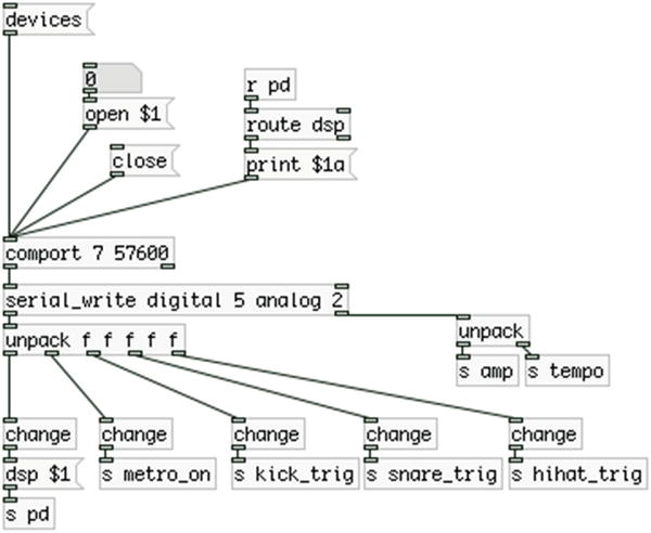
Figure 4-6. Contents of the arduino_stuff subpatch
The sound_tabs Subpatch
The next subpatch is sound_tabs, which is shown in Figure 4-7. In this subpatch, we’re storing the audio samples for our drum machine. I have downloaded three samples from freesound.org, a kick-drum, a snare-drum, and a hi-hat sample, which I have named “kick,” “snare,” and “hihat,” respectively. Inside the Pd patch folder, I’ve created a folder called sounds, and I put all three samples in there. All this is necessary so that Pd knows where to look for these audio samples, to load them to tables.
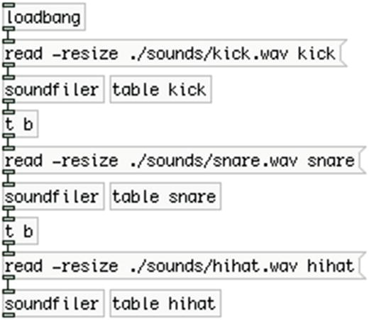
Figure 4-7. Contents of the sound_tabs subpatch
Since this is going to be a fixed interface, it’s nice not having to load your audio samples manually. To do this, we’re using [loadbang], which sends a band as soon as the patch is loaded, which goes to a message that reads “read -resize ./sounds/kick.wav kick”. This messages is sent to [soundfiler], which will load the sample to the table it is told to. The message tells [soundfiler] to “read” the file called kick.wav (the file extension, .wav, must be included), which is located in the sounds directory, which directory is located in the current directory. This is the ./sounds/kick.wav part of the message. The dot means the current directory, and then we’re being navigated to the sounds directory to retrieve the kick.wav file. This is Unix syntax, which you saw in Chapter 3, when we were navigating through the Linux system in the Raspberry Pi. This syntax will work in Windows too, even though it is not Unix. The message also contains the -resize flag, before the path to the audio file, which tells [soundfiler] to resize the table it will store the audio file to, to the size of the file. The last word in the message is the name of the table. To put it all together, when you want to load an audio file to a table, the message sent to [soundfiler] should contain the read command with the -resize flag, then the path to the audio sample, and lastly, the name of the table to load the file to.
Next to [soundfiler]. You can see the table that the audio file will be loaded to. Make sure that you give it the same name as the last word in the message. We could have used arrays, but we don’t really need to look at the graph of the audio file, so we prefer to use [table] instead. If you click [table] (in a locked patch), you’ll be able to see the graph of the file.
[soundfiler] outputs the number of samples the audio file consists of. Don’t confuse the word sample with the way we use it for an audio file. In computer music, a sample is a discrete value representing the amplitude of sound. It is confusing when the same word is being used for a short audio file, like one kick of a kick drum. Since the drum machine we’re building is based on audio files, we’re using the word sample to refer to these files, as it is widely used this way, but the samples number [soundfiler] outputs, concern the discrete amplitude values. This number [soundfiler] outputs is necessary when we use [tabread~] to read the audio file from the table. In this patch, though, we’re using [tabplay~], so we don’t really need it. [tabplay~] only takes a bang to play the contents of a table. The advantage of this is that it is much easier to set up a playback patch, but the disadvantage is that we can’t really change various aspects of the playback of the audio file, like the speed, the start and end positions of the table, or the playback direction. We’ll use [tabread~] in other chapters in this book. So, we might not need the value output by [soundfiler], but we do need to bang the next message to load the next audio file to the next table, once we’re done with the current audio file. To do this, we’re connecting the outlet of [soundfiler] to [t b], to convert the outgoing value to a bang, which will bang the message below it. This whole procedure is being done in a chain, resulting in the automatic load of all audio samples when the patch loads.
The audio_out Subpatch
The next subpatch is audio_out, which is shown in Figure 4-8.
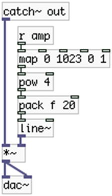
Figure 4-8. Contents of the audio_out subpatch
Here you see the first [receive], which takes input from [s amp], which comes from the first potentiometer, and it’s located in the arduino_stuff subpatch (actually all [send]s are located there). We also have the [catch~], which takes audio from the three [throw~]s in the parent patch. We could have used [inlet~] instead and connect the output of all [tabplay~]s to it, but [throw~]/[catch~] makes the patch a bit more tidy. It might increase the CPU a bit, but the audio processing done in this patch is very small, so CPU is not a problem. Again, we’re mapping the 10-bit range of the potentiometer to a range from 0 to 1, but this time we’re sending the output to [pow 4]. This object raises the value that comes in its left inlet to a power set either via an argument, or via the right inlet. In this case, we’re raising the value to the 4th power. We do this to make the audio fade in and out smoother, more like in audio equipment, like mixers for example. Figures 4-9 and 4-10 show a linear and an exponential curve respectively, the latter made by raising an incrementing value from 0 to 1, to the 4th power (you’ll see [loop] in action later). Our perception of loudness is logarithmic, and using an exponential curve to control it, makes things sound more natural.
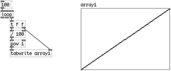
Figure 4-9. Linear curve
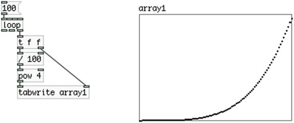
Figure 4-10. Exponential curve by raising values to the 4th power
The next subpatch is metronome, which is shown in Figure 4-11. This is the heart of the sequencer of our drum machine. [metro] is an object that outputs bangs at a specified time interval, in milliseconds. This interval can be set either via an argument, or via the right inlet. Any non-zero value in its left inlet will start it, and a zero will stop it. [r tempo] takes input from the second potentiometer, which we map to a range between 40 and 240. We send that to [i ] to get the integral part of the value (“i” stands for integer) and we multiply it by 4. This will be our tempo in BPMs, but we’re splitting each bit to four, because we want to bang 16-notes and not quarter notes, so we need four bangs per beat. Then we send that value to an abstraction called BPM2ms. This is quite similar to the [Hz2ms] abstraction we made in Chapter 1; it is shown in Figure 4-12.
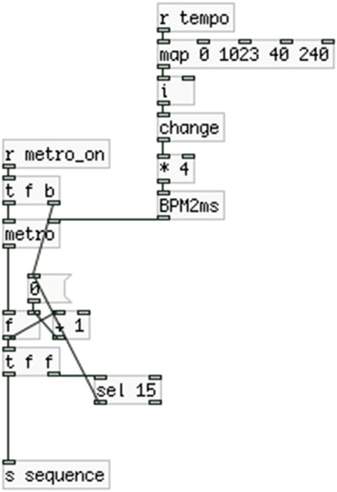
Figure 4-11. Contents of the metronome subpatch
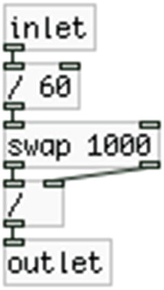
Figure 4-12. [BPM2ms] abstraction
I’m not going to explain how this abstraction works, as it is pretty simple, but try to understand it yourself (mind that [swap 1000] has both its outlets connect to both inlets of [/ ]). Since BPM is a more musical measure unit, it’s better to use it in our interface. [metro] takes in milliseconds, so we need to do the conversion before we send the potentiometer value to the right inlet of [metro], otherwise, the tempo would rise as the potentiometer’s value fell. In Figure 4-11, you see that before the BPM value goes to the multiplication object, it goes through a [change]. The analog pins of the Arduino tend to have a bit of noise. Since we’re reducing the resolution of the potentiometer by mapping its value to a much smaller range, we also reduce the noise, making it much more stable. I have also mentioned that division in computers is quite CPU-intensive, so it’s better to avoid it when you can. Since the potentiometer’s output have become more steady, we can use [change] to make sure that the its value will be sent to [BPM2ms] only when it is changed, so we can avoid doing these two division shown in Figure 4-12 every time we receive input from [comport].
In Figure 4-11, below [metro], you can see a simple incrementing counter. This counter sends its values both to [sel 15] and to [s sequence]. [sel 15] will output a bang out its left outlet whenever it receives the value 15. This bang goes to the message “0”, which goes to the right inlet of [f ]. So, whenever our counter reaches 15, its internal value will be updated to 0, and it will start again (the right inlet of [f ] is cold and will only store the value and won’t output it, it will only be output when [f ] receives the next bang). We’re building a 16-step sequencer here, so we need to update our counter after 16 steps, and since the counter starts counting from 0, the last step will be step number 15. [s sequence] will send the counter’s value to each [tabplay~] object in the parent patch. Finally, [metro] will be triggered when [r metro_on], the second switch in our circuit, sends a 1.
The set_sequence Subpatch
The next subpatch is set_sequence, which is shown in Figure 4-13. In this subpatch, we can set the sequence for each audio file.
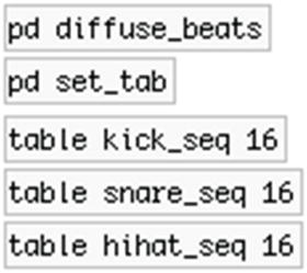
Figure 4-13. Contents of the set_sequence subpatch
The diffuse_beats Subpatch
The first subpatch is [pd diffuse_beats] , which you can see in Figure 4-14. This subpatch takes input from the toggle matrix of the parent patch. To achieve this you have to go to the parent patch and change the properties of each toggle. Right-click the top-left toggle and select Properties. You should get a window like in Figure 4-15. Go to the Send symbol: field and type tog0, like in Figure 4-14, and in the Receive symbol: below, type r-tog0. Do this for every toggle, but increment the number, so the second from top-left toggle should get the symbols tog1 and r-tog1, the third from top-left should get tog2 and r-tog2, and so forth. You can use any name you like for these toggles, but using consistent names that don’t need much explanation is a very good programming practice. When done with the top line of toggles, go to the line below and again start from left to right. You should end up with the bottom-right toggle, which should get the symbols tog15 and r-tog15. This is a bit of a cumbersome procedure, but it will facilitate the use of the patch a lot. Also notice that we start numbering the toggles from 0, and we end with 15, instead of 16. This is because in programming, we usually start counting from 0, and since we’re going to reference these toggles with some automation processes, it’s easier if we do it this way, instead of numbering them from 1 to 16.
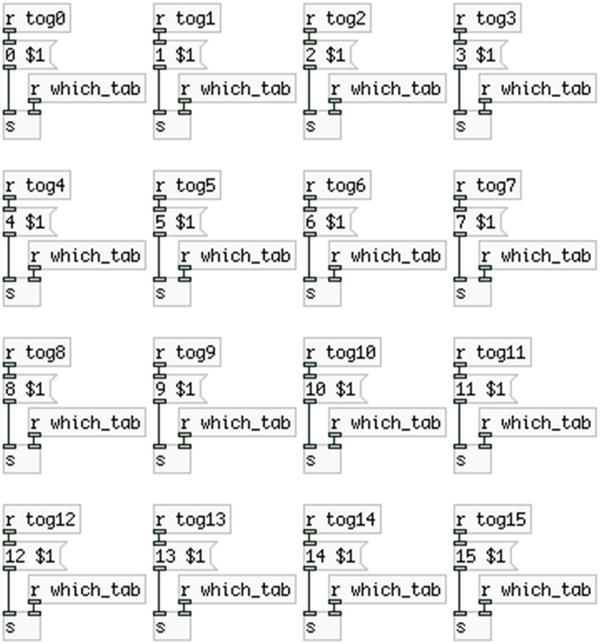
Figure 4-14. Contents of the diffuse_beats subpatch
Now let’s go back to the [pd diffuse_beats] subpatch. Even though it looks like a lot of work to build this patch, it is actually quite easy if you use the duplicate feature. Go ahead and make the top-left set of objects, [r tog0], [r which_tab], [s ], and the “0 $1” message, and connect them like in Figure 4-15. Then select them all and hit Ctrl/Cmd+D, for duplicate. Press Shift+up arrow to bring the duplicated objects to the same height with the original ones, and use Shift+right arrow to move them to the right. Select both sets of objects and again duplicate them. Again, use Shift and arrows to move them. Now you should have four sets of objects, all connected as they should. Now select all four and duplicate them to get eight sets. Lastly, select all eight sets and duplicate them, and you’ll get sixteen sets.
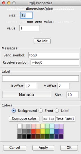
Figure 4-15. Toggle’s properties
All you need to do now is change the numbers in [r tog0] and in the message “0 $1”, replicating Figure 4-14. These sets represent the position of the toggles of the parent patch, so make sure that their names match along with the names set to the toggles via their properties. [s ] will take a symbol with the name of the table to write to, which will be one of the [table]s in Figure 4-13. The messages “0 $1”, “1 $1”, and so forth. will write the value received by $1 to the index set by the value 0, 1, and so forth. What actually happens here is that [r tog0] will get a value from the corresponding toggle, and it will write it to the first index (index 0) of the table set by [r which_tab]. [r tog1] will get a value from the corresponding toggle and it will write it to the second index of the table, and so on. [r which_tab] receives a symbol from the set_tab subpatch you see in Figure 4-13, which is shown in Figure 4-16. The 1s and 0s that we’ll write to the sequence tables will be read in the parent patch by the [tabread] objects, where a 1 will trigger the audio file read by [tabplay~]. This way we can use the counter to trigger each audio file at the location we want. This is how a sequencer works.
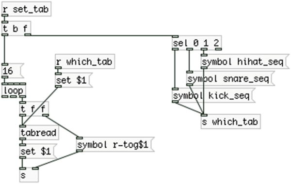
Figure 4-16. Contents of the set_tab subpatch
The set_tab Subpatch
This subpatch takes input from the Vradio shown of the parent patch. We’ve set the number of cells of the radio via its properties, in the number: field, which by default is 8, and we set it to 3 (right-click it and select Properties). Also, we’ve used comments next to each cell of the Vradio to specify what each cell will select (kick, snare, and hihat). In Figure 4-16, we receive that value and we send it to [sel 0 1 2], which will bang the corresponding symbol. In Pd, you can create a symbol from a message by prepending the word symbol. These symbols are the names of the tables in Figure 4-13, which will store the sequences for each audio file, and they are being sent to [s which_tab], which we receive with [r which_tab] in Figure 4-14. This way we can set the table to write our sequences in an easy-to-use way.
Once the table has been set, we run a loop that will read the values stored in the selected table, and will set each value to the corresponding toggle of the parent patch. [loop] is an abstraction found the in “miscellaneous_abstractions” GitHub page, already provided. Check its help patch to see how it works. [tabread] takes a message that is formed according to what is received in [r which_tab], which is a symbol with the name of the table. The message “set table_name” sent to [tabread], sets the table to read from. So, if we click the first cell of the Vradio in the parent patch, [tabread] will read from [table kick_seq 16]. [loop] will output 16 incrementing numbers starting from 0, ending in 15. These numbers will first go to the “symbol r-tog$1” message, which is sent to the right inlet of [s ]. This will set the destination of [s ], to each toggle of the parent patch, sequentially (remember, we’ve set their Receive symbol: fields to r-tog0, r-tog1, etc.). Then the values go to [tabread], which will output the value at that index. So, the value at index 0 of [table kick_seq 16] will go to the toggle that receives from “r-tog0”, the value at index 1 will go to the toggle that receives from r-tog1, and so forth. Sending a value with the message “set”, only sets the value to the toggle, and doesn’t produce any output. If you omit to put the message “set $1”, whatever you send to each toggle, will be output, and again written to the table. In this case this won’t cause an infinite loop, but in general, when you only want a toggle to project its value, it’s good practice to use the message “set” to avoid possible bugs. The mechanism of the set_tab subpatch projects the values stored at each table as soon as you select it. If you omit the loop in this patch, you’ll realize that whenever you’ll want to write a sequence to a new table, what you’ll get in the toggles will be the values of the previous table, which is not efficient at all. You can try for yourself to see why that is. To create your sequences, in the set_sequence subpatch, select the audio file you want from the Vradio, and click the toggles where you want that file to be triggered in the sequence.
Concluding the Patch and Explaining the Data received from the Arduino
The patch we’ve built is rather complex, and yet it is a simple drum machine. This is a good demonstration of programming, since you can see that even the simplest things in computers need quite some work, when we program them from scratch. Still, the advantage of programming is that you can build unique interfaces and projects that don’t exist in the market, as they are tailored to one person’s needs. Now let’s go back to Figures 4-5 and 4-6, the parent patch and the arduino_stuff subpatch. In the arduino_stuff subpatch, you see that the first switch controls the DSP state of Pd. The second goes to [s metro_on], which is sent to the metronome, inside the metronome abstraction. Whenever this switch is in the ON position, the drum machine will play the sequences stored in the set_sequence subpatch, with the tempo set by the second potentiometer. Whenever it is in the OFF, position, the sequence won’t play, but you’ll be able to trigger each audio file with the three push buttons of your circuit (we haven’t built the circuit yet, but I’ll explain it further on). In the arduino_stuff subpatch you can see three [send]s, [s kick_trig], [s snare_trig], and [s hihat_trig]. These take input from the three push buttons of the circuit, and they are sent to the parent patch. Each [receive] in the parent patch goes to [sel 1], so when you press a button, [sel 1] will output a bang, and [tabplay~] will play the audio file stored in the table it reads from. You can actually trigger the audio files manually, even when the sequence is playing. Finally, we receive input from Pd with [r pd], about the DSP state, which is sent to the Arduino, to control an LED that will indicate the DSP state.
Arduino Code for Drum Machine Patch
Let’s now move on to the Arduino sketch, shown in Listing 4-2.
This sketch is a modified version of the serial_write.ino sketch that goes along with the help patch of the [serial_write] Pd abstraction. There’s really not much to explain here. As with the previous Arduino sketch, in lines 2 and 4 we set constants that will set the size of the array we’ll send to the serial line. This time we’re using the write function instead of print, so we can send all the values in one function call. In line 6, we set the number of digital outputs, which is only one, and in line 11, we assemble the constants of lines 2 and 4, to set the size of the array we’ll send to the serial line. Remember that write sends bytes, and the analog pins of the Arduino have a 10-bit resolution, therefore we need to split them to two, and reassemble them back in Pd. For this reason we need two bytes for each analog pin, and one for each digital (these will be either 1 or 0), plus one unique byte to denote the beginning of the data stream.
In the setup function, we set the modes of the digital pins and we begin the serial communication at a 57600 baud rate. In the loop function we first set the unique byte to the beginning of the array, and then we define an index offset for writing the rest of the values to the array. If you can’t remember how this works and why we need to do it this way, go back to end of Chapter 2. Then in lines 29 to 45 we check whether we have input from Pd, to control the DSP LED. Afterward, we read and store the digital input values (remember in the Pd patch, we’ve set the digital pins first in the arguments of [serial_write]. The order of these arguments should be aligned with the order of the reading on pins in the Arduino sketch), and then the analog ones. Once we’re done, we send the whole array to Pd.
Circuit for Arduino Code
Now let’s check the circuit for this project, which is shown in Figure 4-17.
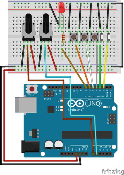
Figure 4-17. Simple drum machine circuit
We follow the same philosophy concerning connections, so make sure that you connect the potentiometers from analog pin 0 onward, and the switches and push buttons from the digital pin2 onward. The LED should go to the first digital pin after the digital inputs. This helps automating some routines in the Arduino sketch, like setting the mode of the digital pins, and reading the correct pins; otherwise, we would need to set the pin numbers explicitly, and the for loops wouldn’t be so simple.
Go ahead and store some sequences to the Pd patch, and start playing! One drawback of the Pd patch is that we cannot save the sequences we write, so every time we open the patch we need to create them anew. A simple way is to go to the toggle’s properties and click the No init button, which will become Init. This way the patch will save the last value each toggle had before the patch was closed. If we want to store all sequences, we must save the contents of the [table]s to text files, but this adds some complexity, and since this is just an introductory project, we won’t deal with it. If you want to check for yourselves, check [textfile]. An easy work around is to use arrays instead of [table]s, because in the array’s properties we can set it to save its contents. Having the graphs of the arrays for the sequences is not so elegant, and we really don’t need to look at them, as the toggles project the sequences in a much more user-friendly way. At the time of writing (September 2015), the latest Pd-vanilla has introduced the [array] object, which can save its contents, much like the array can. Unfortunately, this object doesn’t exist in Pd-extended, so we must go for one of the other solutions mentioned.
Drum Machine and Phase Modulation Combination
Before we close this chapter, let’s combine the two interfaces we built. It shouldn’t be very complicated to do this, still there are some details I’ll need to explain thoroughly. This time we’ll start with the Arduino sketch. We’re going to use the print function to send data to Pd, so we can retrieve it with objects like [r drum_machine_switches], which should make things self-explanatory.
Arduino Code
Listing 4-3 shows the Arduino sketch, which is the longest we’ve written so far. This is because we want to send groups of values separately, for example, one group will consist of the switches for the drum machine, another group will consist of the switches for the phase modulation, and so on. Write the code in Listing 4-3 to the Arduino IDE and check the circuit of the project, shown in Figure 4-18, as I explain how the code functions.
This sketch is long only because we have things being repeated. Lines 1 to 7 define some constants that hold the number of pins for each group. We’re separating switches from push buttons and potentiometers into different groups, one of each for the drum machine and one for the phase modulation part of the patch. This makes a total of six groups, and lastly we define a variable for the LED, which will indicate the DSP state. Lines 10 to 15 define offsets for the pins of each group, according to the number of pins used by each group. The drum machine potentiometer group, doesn’t need an offset, because it starts from analog pin 0. The drum machine switch group needs an offset, because even though it’s the first digital pin group, we start using digital pins from 2 onward. Combine this part of the sketch with the circuit in Figure 4-18. In the circuit, switches, buttons, and potentiometers, are being grouped by being placed close to each other. Check which pin each switch, button, or potentiometer of each group uses, and try to understand how these offsets will be helpful to use. Lines 18 to 23 define arrays for each value group.
In the setup function, we set the mode of all digital pins used. Here is the first part where we use the offsets we’ve set in lines 10 to 15. We need the variable i of the for loop to start from 0, so the loop will run as many times as we need, using the constant that stores the number of pins of each group (drum_machine_switches for example, in line 27). Since i will start from 0, we need the pin offsets so that the pinMode function will use the correct pin. In the loop function, the first thing we do is check if we have input in the serial line, and use that to control the DSP LED. This happens in lines 44 to 57. Afterward, in lines 60 to 72, we read and store the values read from each group, starting with the potentiometers, then reading the switches, and finally the push buttons of each group, alternately. Finally, in lines 75 to 115, we print the values of each group to the serial line, each time using an appropriate tag. Notice that we don’t need to print the groups in some specific order, since all values have already been grouped and stored in different arrays. It might have been easier to use the write function instead of print, and save ourselves from quite some code writing. If we did that, we would be receiving all values together and we would have to split them in the Pd patch. Now we’ll be receiving each group according to its tag, using [receive], which will make things easier. I can’t say that one technique is superior to the other; they’re just different approaches. I’m presenting both approaches in this chapter so that you can see which one works best for you.
Arduino Circuit
As you can imagine, the circuit is a combination of the circuits of the two previous interfaces. It is shown in Figure 4-18.
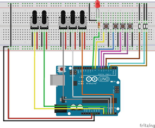
Figure 4-18. Drum machine-phase modulation circuit
Pd Patch for Drum Machine-Phase Modulation Interface
Now let’s check the Pd patch. It is obviously a combination of the two previous patches, but it has some enhancements. Figure 4-19 illustrates it.
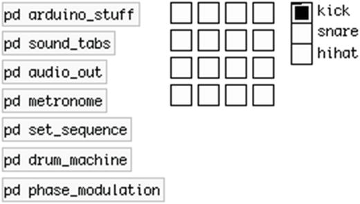
Figure 4-19. Drum machine-phase modulation patch
Like with the previous interface, we’ve put most of the stuff in subpatches to make things clear. The subpatches sound_tabs, audio_out, and set_sequence, are the same with the previous project of this chapter, so I’m not going to explain them here. The arduino_stuff and metronome have changed a bit, and we now have two new ones, drum_machine and phase_modulation.
The arduino_stuff Subpatch
Figure 4-20 illustrates the contents of arduino_stuff.
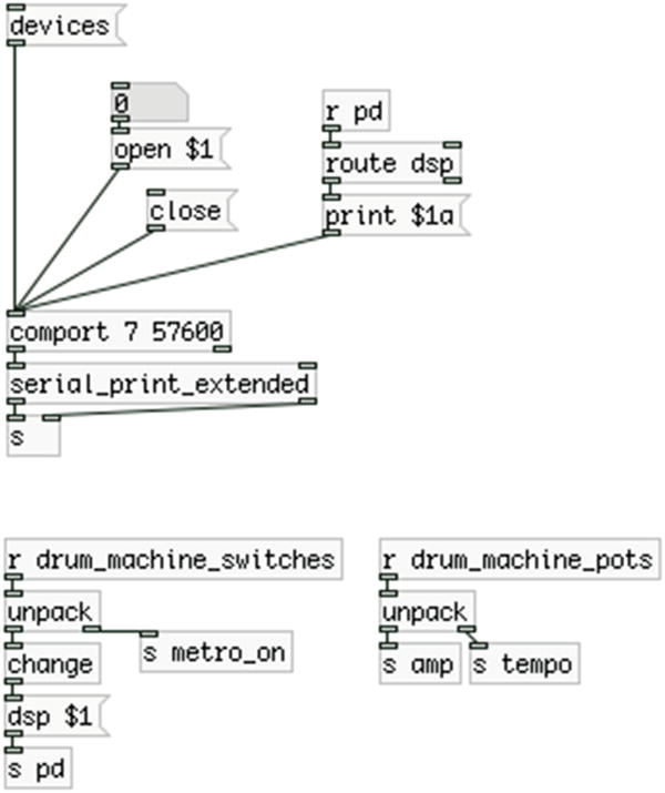
Figure 4-20. Contents of the arduino_stuff subpatch
Here we send the bytes [comport] outputs to [serial_print_extended], which sends them to [s ]. Below we receive two of the value groups, drum_machine_switches and drum_machine_pots, which unpack the values of their groups and diffuse them using [send]s. The first switch controls the DSP, and the second controls [metro], which is in the metronome subpatch. The first potentiometer controls the overall amplitude, and the second the BPMs of the metronome. The first switch and the first potentiometer don’t really belong to the drum machine group, but we’ve left them there, from the previous interface.
The metronome Subpatch
Figure 4-21 illustrates the contents of the metronome subpatch. This subpatch hasn’t changed a lot, the only difference is that we’re sending the BPM value both to [metro], and to [s env_dur]. The latter will control the duration of an amplitude envelope for the phase modulation, in the phase_modulation subpatch.
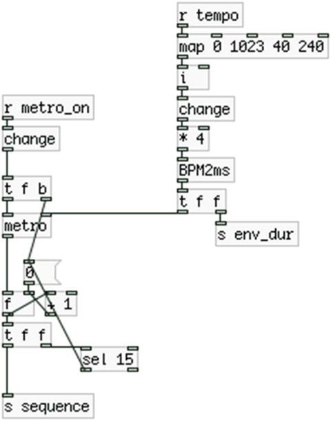
Figure 4-21. Contents of the metronome subpatch
The drum_machine Subpatch
Figure 4-22 illustrates the contents of the drum_machine subpatch. This is the main part of the parent patch of the previous interface. Only two things have changed here. One is the amplitude attenuation of each audio file. Now every [tabplay~] is being multiplied by 0.25, instead of 0.33, because we have the phase modulation part as well, so we have four different audio sources in total. Multiplying each one by 0.25, makes sure that they’ll never exceed 1, even if they are all triggered together. The other thing that has changed is that we have removed the [r kick_trig], [r snare_trig], and [r hihat_trig] objects, because we’re now receiving the drum machine push-button values straight in this subpatch. After unpacking them, we send each to a [change], so that their values will be output only when they’re changed.
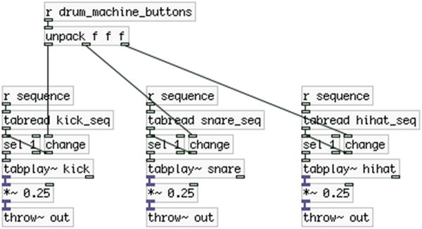
Figure 4-22. Contents of the drum_machine subpatch
The phase_modulation Subpatch
Finally, Figure 4-23 illustrates the contents of the phase_modulation subpatch. The bottom-left part of the patch is copied from the patch of the first interface we built in this chapter. This time we’re using an amplitude envelope made with the [ggee/envgen] external object (the GUI in Figure 4-23). In the left part of the patch, you see a [r phase_mod_pots], which, as its arguments states, receives the values from the potentiometers for the phase modulation. We’re unpacking the list of values and sending them to the carrier frequency, the modulator frequency, and the index. We map the value for the index to the range from 0 to 2, using the [map] abstraction, like we did before. What I need to explain in detail is the right part of the subpatch, where we have the envelope for the amplitude. In Figure 4-23 I have made some sort of an ADSR envelope (the sustain part is also decaying here). Above [ggee/envgen] there is a [r sequence] that receives the sequencer counter, but converts the counter values to two bangs with [t b b]. The first bang (from the right outlet), goes to [f ]. [f ] stores the value from the fourth push button, which is received via [r phase_mod_buttons].
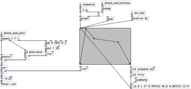
Figure 4-23. Contents of the phase_modulation subpatch
When a new value from the sequencer counter comes in, it will bang [f ], and its value will go to the right inlet of [spigot]. [spigot] works like a gate. If it receives any non-zero value in its right inlet, it will let anything that comes in its left inlet through. If it receives a zero in its right inlet, it will block whatever comes in its left inlet. So, when we keep the button pressed, [spigot] will let the second bang of [t b b] through, which will bang the envelope, so we’ll hear the phase modulation. As long as we keep the button pressed, we’ll keep on triggering the sound of this subpatch with every new count of the sequencer. As soon as we release the button, we’ll stop triggering the envelope and we won’t get the subpatch’s sound. This is designed this way so that the phase modulation is synced with the drum machine. Remember, in the metronome subpatch shown in Figure 4-21, we send the BPM value converted to milliseconds to a [s env_dur]. In Figure 4-23, you see the [r env_dur], which goes into the message “duration $1”. This will set the duration of the envelope to exactly the same length of one bit of the metronome. So, even if we keep the button pressed and we trigger the phase modulation sound on every beat, [ggee/envgen] will have enough time to complete its envelope.
On the bottom-right part in Figure 4-23, we connect the second outlet of [ggee/envgen] to [list prepend set], and then to [list trim] and to a message. Don’t type the values you see in the message of the figure, just leave it blank. Above [ggee/envgen] there is a message “dump.” If you click it, [ggee/envgen] will output the values of its graph out its right outlet. To save our envelope, we store these values to a message that we bang with [loadbang] and send it to [ggee/envgen]’s inlet, so it can create the same envelope by itself. [list prepend set] takes in a list and prepends the last argument, in this case “set”. If we send the message “set something” to an empty message, the word “something” will be printed in the empty message, try it. [list trim] trims the “list” selector off from a list, which has been added by [list prepend set]. If we omit [list trim], what will come out from [list prepend set] will be “list set” along with the values from [ggee/envgen], and the empty message won’t understand it. Trimming out “list” from the list will result in the message “set” along with the values of [ggee/envgen], and this way the values will be saved in the message. Go ahead and create an envelope (make any kind of graph you like in [ggee/envgen]) and click [dump]. You’ll immediately see some values in the empty message. Save your patch, and the next time you’ll open it, you’ll see your envelope still there.
The modulator Subpatch
The last thing to mention about this patch is the modulator subpatch of the phase_modulation subpatch, which is shown in Figure 4-24. This is essentially the same subpatch with the first interface of this chapter, only instead of a [r choose_waveform] in the top-right part of it, there’s a [r phase_mod_switches], which receives the switch value for the phase modulation straight from the [serial_print_extended] abstraction. Again, we’re sending the value to [change –1] so it will give output even if we start the patch with the switch to the OFF position, as we need to select the type of the modulator oscillator right away.
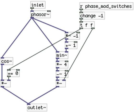
Figure 4-24. Contents of the modulator subpatch
This concludes the description of this interface. We extensively used the print function along with the [serial_print_extended] abstraction to make the Pd patch a bit easier to make and understand. It’s up to you what kind of approach you’ll take for your own projects. Go ahead and play with this interface, it should be fun!
Conclusion
In this chapter, we went through the process of creating a musical interface. The three interfaces made here might not be appealing to everyone, but they server as a generic platform on top of which you can build many different kinds of interfaces. We focused on the two different techniques for communication between the Arduino and Pd, which we have been introduced to in Chapter 2, showing the advantages and disadvantages of each. You should pick the technique that fits your needs best, there’s no definite rule as to which technique is better over the other.
We have also developed both our Pd patching and our Arduino programming in this chapter. As we move further into this book, things will get even more advanced. This should apply mostly to the Pd patching, as the Arduino code we’ll be using will most of the time follow the lines of the [serial_print_extended] and the [serial_write] abstractions. In some cases, we’ll be building complex interfaces where the Arduino code will also differ from what we’ve already seen, but that won’t happen often. Our Pd patching will definitely grow larger, as we’ll need to create complex patches to express our musicality.
Up until now, we’ve used oscillators and sound files to create sound. The oscillator is the basis of electronic music, but in some cases, we might want to process live input, from an instrument for example. In the next chapter, we’ll build a synthesizer using a MIDI keyboard, so again, we’ll use oscillators (along with filters and envelopes) to create our sounds, but in the chapter after that we’ll start using live input and we’ll learn different ways to manipulate that input to create something interesting. Chapters will alternate between the use of oscillators, audio files, and live input, in an attempt to meet as many needs as possible. Even if the interfaces that we’re building in this book aren’t something you’re really interested in, if you want to make electronic music by building your own interface, you’ll find very useful information and techniques that will prove helpful in creating your own ideas.
This chapter finalizes all the introductory material, from a technical point of view, but also from a creative point of view. Now you should be ready to start creating projects that utilize musical ideas to a great extent; projects that you should be able to use even at a professional level. Next, a keyboard synthesizer using a MIDI keyboard, Arduino, and Pd.
______________________
1It is said that “good” index values for phase modulation are between 0 and 1, but higher values can produce nice results.