
Chapter 3. Scaling
Running redundant copies of services is important for at least two reasons.
The first reason is to achieve high availability with the application, tied with the fact that processes—and whole machines—occasionally crash. If only a single instance of a producer is running, and that producer crashes, then consumers are unable to function until the crashed producer has been relaunched.
Another reason is that there’s only so much throughput that a particular Node.js instance can handle. For example, depending on the hardware, the most basic “Hello World“ example that can be built using Node.js might have a throughput of around 40,000 requests per second (R/S). Once an application begins serializing and deserializing payloads or doing other CPU intensive work, that throughput is going to drop by orders of magnitude. Offloading work to additional processes helps prevent a single process from getting overwhelmed.
There are a few tools available for splitting up work. “The Cluster Module” looks at a built-in module that makes it easy to run redundant copies of application code on the same server. “Reverse proxies with HAProxy” considers how to run multiple redundant copies of a service using an external tool—one that lets you run copies on different machines. And finally, “SLA and Load Testing” looks at how to use benchmarks to understand the load that an application can handle, as well as the importance of defining an SLA.
The Cluster Module
Node.js provides the cluster module to allow running multiple copies of a Node.js application on the same machine, dispatching incoming network messages to to the instances. This module is pretty similar to the child_process module which provides a fork() method for spawning Node.js sub processes; the main difference is the mechanism for routing incoming requests.
The documentation for cluster includes a single Node.js file that loads the http and cluster modules, has an if statement to see if the script is being run as the master, forking off some worker processes if true. Otherwise, if it’s not the master, it creates an HTTP service and begins listening. This example code is both a little bit dangerous and a little bit misleading.
A Simple Example
The reason the code is dangerous is that it promotes loading a lot of potentially heavy and complicated modules within the parent process. The reason it’s misleading is that the example doesn’t make it obvious that multiple, separate instances of the application are running and that things like global variables cannot be shared. For these reasons I prefer to use a modified example like the one in Example 3-1.
Example 3-1. recipe-api/producer-http-basic-master.js
#!/usr/bin/env nodeconstcluster=require('cluster');console.log(`master pid=${process.pid}`);cluster.setupMaster({exec:__dirname+'/producer-http-basic.js'});cluster.fork();cluster.fork();cluster.on('disconnect',(worker)=>{console.log('disconnect',worker.id);}).on('exit',(worker,code,signal)=>{console.log('exit',worker.id,code,signal);// cluster.fork();}).on('listening',(worker,{address,port})=>{console.log('listening',worker.id,`${address}:${port}`);});

The cluster module is needed in the parent process.

Override the default application entry point of
__filename.
cluster.fork()is called once for each time a worker needs to be created. This code produces two workers.
Several events that cluster emits are listened to and logged.

Uncomment this to make workers difficult to kill.
The way cluster works is that the master process spawns worker processes in a special mode where a few things can happen. In this mode, when a worker attempts to listen on a port, it sends a message to the master. It’s actually the master that listens on the port. Incoming requests are then routed to the different worker processes. If any workers attempt to listen on the special port 0 (used for picking a random port), the master will listen once and each individual worker will receive requests from that same random port. A visualization of this master and worker relationship is provided in Figure 3-1.
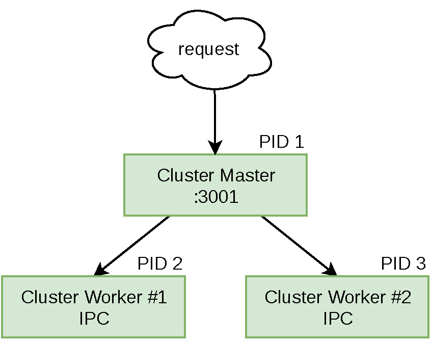
Figure 3-1. Master worker relationships with cluster
Typically no changes need to be made to an application that will serve as the worker—the recipe-api/producer-http-basic.js code will work just fine. Now it’s time to make a few requests to the server. This time, execute the recipe-api/producer-http-basic-master.js file instead of recipe-api/producer-http-basic.js file. In the output you should see some messages resembling the following:
master pid=7649
Producer running at http://127.0.0.1:4000
Producer running at http://127.0.0.1:4000
listening 1 127.0.0.1:4000
listening 2 127.0.0.1:4000
Now there are three running processes. This can be confirmed by running the following command, where <PID> is replaced with the process ID of the master process, in my case 7649:
$brew install pstree# if using macOS$pstree <PID> -p -a
A truncated version of the output from this command when run on my Linux machine looks like this:
node,7649 ./master.js
  ├─node,7656 server.js
  │   ├─{node},15233
  │   ├─{node},15234
  │   ├─{node},15235
  │   ├─{node},15236
  │   ├─{node},15237
  │   └─{node},15243
  ├─node,7657 server.js
  │   ├─ ... Six total children like above ...
  │   └─{node},15244
  ├─ ... Six total children like above ...
  └─{node},15230
This provides a nice visualization of the parent process, displayed as ./master.js, as well as the two child processes, displayed as server.js. It also displays some other interesting information if run on a Linux machine. Note that each of the three processes shows six additional child entries below them, each labelled as {node}, as well as their unique process IDs. These entries suggest multithreading in the underlying libuv layer. Note that if you run this on macOS you will only see the three Node.js processes listed.
Request Dispatching
By default, on macOS and Linux machines, the requests will be dispatched Round-robin to the workers. On Windows, requests will be dispatched depending on which worker is perceived to be less busy. You can make three successive requests directly to the recipe-api service and see this happening for yourself. With this example requests are made directly to the recipe_api, since these changes won’t affect the web-api service. Run the following command three times in another terminal window:
$curl http://localhost:4000/recipes/42# run three times
In the output you should see that the requests have been cycled between the two running worker instances:
worker request pid=7656
worker request pid=7657
worker request pid=7656
As you may recall from Example 3-1, some event listeners were created in the recipe-api/master.js file. So far the listening event has been triggered. This next step will trigger the other two. When you made the three HTTP requests, the PID values of the worker processes were displayed in the console. Go ahead and kill one of the processes to see what happens. Choose one of the PIDs and run the following command:
$kill<pid>
In my case I ran kill 7656. The master process will then have both the disconnect and the exit events fire, in that order. You should see output similar to the following:
disconnect 1
exit 1 null SIGTERM
Now, go ahead and repeat the same three HTTP requests:
$curl http://localhost:4000/recipes/42# run three times
This time, each of the responses are coming from the same remaining worker process. If you then run the kill command with the remaining worker process, you’ll see that the disconnect and exit events are called, and that the master process then quits.
Notice that there’s a commented call to cluster.fork() inside of the exit event handler. Uncomment that line, start the master process again, and make some requests to get the PID values of the workers, then run the kill command to stop one of the workers. Notice that the worker process is then immediately started again by the master. In this case the only way to permanently kill the children is to kill the master.
Cluster Shortcomings
The cluster module isn’t a magic bullet. In fact, it is often more of an anti-pattern. Usually it makes sense to use another tool to manage running multiple copies of a Node.js process. This includes things like visibility into process crashes and granularity of choosing deployment size. Sure, you could build in application support for scaling the number of workers up and down, but that’s better left to an outside tool. [Link to Come] looks into doing just that.
This module is mostly useful in situations where an applications is bound by the CPU, not by I/O. This is in part due to JavaScript being single threaded, and also due to libuv being so efficient at handling asynchronous work with the event loop. It’s also pretty fast due to the way it passes incoming requests to a child process. In theory this is faster than using a reverse proxy.
Tip
Node.js applications can get complex. Processes often end up with dozens, if not hundreds, of modules that make outside connections, consume memory, or read configuration. Each one of these operations can expose another weakness in an application that can cause it to crash.
For this reason it’s better to keep the master process as simple as possible. Example 3-1 shows that there’s no reason to load an HTTP framework or really any third-party modules or consume another database connection. Logic could be built into the master to restart failed workers, but the master can’t be restarted as easily.
Another caveat of the cluster module is that it’s essentially operates at Layer 4, at the TCP/UDP level, and isn’t necessarily aware of Layer 7 protocols. Why might this matter? Well, with an incoming HTTP request being sent to a master and two workers, assuming the TCP connection closes after the request finishes, each subsequent request will then get dispatched to a different backend service. However, with gRPC over HTTP/2, those connections are intentionally left open for much longer. In these situations future gRPC calls will not get dispatched to separate worker processes—they’ll be stuck with just one. When this happens you’ll often see that one worker is doing most of the work, and the whole purpose of clustering has been defeated.
This issue with sticky connections can be proved by adapting it to the code written previously in “RPC with gRPC”. By leaving the producer and consumer code exactly the same, and by introducing the generic cluster master from Example 3-1, the issue surfaces. Run the producer master and the consumer, and make several HTTP requests to the consumer, and the returned producer_data.pid value will always be the same. Then, stop and restart the consumer. This will cause the HTTP/2 connection to stop and start again. The round-robin routing of cluster will then route the consumer to the other worker. Make several HTTP requests to the consumer again, and the producer_data.pid values will now all point to the second worker.
Another reason you shouldn’t always reach for the cluster module is that it won’t always make an application faster. In some situations it can simply consume more resources and have either no effect or a negative effect on the performance of the application. Consider, for example, an environment where a process is limited to a single CPU core. This can happen if you’re running on a VPS (Virtual Private Server, a fancy name for a dedicated virtual machine) such as a t3.small machine offered on AWS EC2. It can also happen if a process is running inside of a container with CPU constraints, which can be configured when running an application within Docker.
The reason for a slowdown is because of this: When running a cluster with two workers, there are three single-threaded instances of JavaScript running. However, there is a single CPU core available to run each instance on at a time. This means the operating system has to do more work deciding which of the three processes runs at any given time. True, the master instance is mostly asleep, but the two workers will fight with each other for CPU cycles.
Note
“SLA and Load Testing” looks at benchmarks in much more detail, but for now you can do a quick one just to prove out these performance constraints. If you have access to a Linux machine with multiple CPU cores you can run the remaining examples in this section. Otherwise, just read along.
First off, create a new file for simulating a service that performs CPU intensive work, making it a candidate for using with cluster. This service will simply calculate Fibonacci values based on an input number. Example 3-2 is an example of such a service.
Example 3-2. cluster-fibonacci.js
#!/usr/bin/env node// npm install fastify@2constserver=require('fastify')();constHOST=process.env.HOST||'127.0.0.1';constPORT=process.env.PORT||4000;console.log(`worker pid=${process.pid}`);server.get('/:limit',async(req,reply)=>{returnString(fibonacci(Number(req.params.limit)));});server.listen(PORT,HOST,()=>{console.log(`Producer running at http://${HOST}:${PORT}`);});functionfibonacci(limit){letprev=1n,next=0n,swap;while(limit){swap=prev;prev=prev+next;next=swap;limit--;}returnnext;}
The service has a single route,
/<limit>, where limit is the number of iterations to count.The
Fibonacci()method does a lot of CPU intensive math and blocks the event loop.
The same Example 3-1 code can be used for acting as the cluster master. Recreate the content from the cluster master example and place it in a master-fibonacci.js file next to cluster-fibonacci.js. Then update it so that it’s loading cluster-fibonacci.js, instead of server.js.
The first thing you’ll do is run a benchmark against a cluster of Fibonacci services. Execute the master-fibonacci.js file, and then run a benchmarking command:
$npm install -g autocannon@4$node master-fibonacci.js$autocannon -c2http://127.0.0.1:4000/100000
This will run the Autocannon benchmarking tool (covered in more detail in “Introduction to Autocannon”) against the application. It will run over two connections, as fast as it can, for ten seconds. Once the operation is complete you’ll get a table of statistics in response. For now you’ll only consider two values, and the values I received have been recreated in Table 3-1.
| Statistic | Result |
|---|---|
Avg Latency |
147.05 ms |
Avg Req/Sec |
13.46 r/s |
Next, kill the master-fibonacci.js cluster master, then run just the cluster-fibonacci.js file directly. Then, run the exact same autocannon command that you ran before. Again you’ll get some more results, and mine happen to look like Table 3-2.
| Statistic | Result |
|---|---|
Avg Latency |
239.61 ms |
Avg Req/Sec |
8.2 r/s |
In this situation, on my machine with multiple CPU cores, I can see that by running two instances of the CPU-intensive Fibonacci service, I’m able to increase throughput by about 40%. You should see something similar.
Next, you’ll simulate an environment that only has a single CPU instance available. Later in Chapter 5 you’ll use Docker and can set CPU restrictions there, but for now, just run the application directly on a machine and use the taskset command to force processes to use a specific CPU core.
Run the master-fibonacci.js cluster master file again. Note that the output of the service includes the PID value of the master, as well as the two workers. Take note of these PID values, and in another terminal, run the following command:
# Linux-only command:$taskset -cp0<pid># run for master, worker 1, worker 2
Finally, run the same autocannon command used throughout this section. Once it completes you’ll get some more information provided to you. In my case, I received the results shown in Table 3-3.
| Statistic | Result |
|---|---|
Avg Latency |
252.09 ms |
Avg Req/Sec |
7.8 r/s |
In this case, I can see that using the cluster module, when having more worker threads than I have CPU cores, results in an application that runs slower than if I had only run a single instance of the process on my machine.
The greatest shortcoming of cluster is that it only dispatches incoming requests to processes running on the same machine. The next section looks at a tool that works when application code runs on multiple machines.
Reverse proxies with HAProxy
A reverse proxy is a tool that accepts requests from a client, forwards it to a server, takes the response from the server, and sends it back to the client. At first glance it may sound like such a tool merely adds an unnecessary network hop and increases network latency, but as you’ll see, it actually provides many useful features to a service stack. Reverse proxies often operate at either the L4 layer, such as TCP, or L7, via HTTP.
One of the features it provides is that of load balancing. A reverse proxy can accept an incoming request, and forward it to one of several servers, before replying with the response to the client. Again, this may sound like an additional hop for no reason, as a client could maintain a list of upstream servers and directly communicate with a specific server. However, consider the situation where an organization may have several different API servers running. An organization wouldn’t want to put the onus of choosing which API server to use on a third-party consumer, such as exposing api1.example.org - api9. Instead, such a developer should be able to use api.example.org and their requests should automatically get routed to an appropriate service. A diagram of this concept is shown in Figure 3-2.

Figure 3-2. Reverse proxies intercept incoming network traffic
There are several different approaches a reverse proxy can take when choosing which backend service to route an incoming request to. Just like with the cluster module, the Round-robin is usually the default behavior. Requests can also be dispatched based on which backend service is currently servicing the fewest requests, they can be dispatched randomly, they can even be dispatched based on content of the initial request, such as a session ID stored in an HTTP URL or cookie (commonly referred to as a sticky session ). And, perhaps most powerful, a reverse proxy can poll backend services to see which ones are healthy, refusing to dispatch requests to services that aren’t healthy.
Other beneficial features include cleaning up or rejecting malformed HTTP requests (which can prevent bugs in the Node.js HTTP parser from being exploited), logging requests so that application code doesn’t have to, adding request timeouts, and as was at before, performing gzip compression and TLS encryption. The benefits of a reverse proxy usually far outweigh the cons for all but the most performance-critical of applications. Because of this you should almost always use some form of reverse proxy between your Node.js applications and the internet.
Introduction to HAProxy
HAProxy is very performant open source reverse proxy that works with both Layer 4 and Layer 7 protocols. It’s written in C and is designed to be stable and use minimal resources, offloading as much processing as possible to the kernel instead of in the application. Like JavaScript, HAProxy is event driven and single threaded.
HAProxy is quite simple to setup. It can be deployed by shipping a single binary executable weighing in at about a dozen megabytes. Configuration can be done entirely using a single text file.
Before you start running HAProxy, you’ll first need to have it installed. A few suggestions for doing so are provided in [Link to Come]. Otherwise, feel free to use whatever your preferred methodology is for installing software to get a copy of HAProxy >= v2 installed on your development machine.
HAProxy provides an optional web dashboard that displays statistics for a running HAProxy instance. Create a first HAProxy configuration file, one that doesn’t yet perform any actual reverse proxying, instead it will just expose the dashboard. Create a file named haproxy/stats.cfg in your project folder and add the content shown in Example 3-3.
Example 3-3. haproxy/stats.cfg
frontend inbound
Create a frontend called inbound.
Listen for HTTP traffic on port
:8000.Enable the stats interface.
With that file created you’re now ready to execute HAProxy. Run the following command in a terminal window:
$ haproxy -f haproxy/stats.cfgYou’ll get a few warnings printed in the console since the config file is a little too simple. These warnings will be fixed soon, but HAProxy will otherwise run just fine. Next, in a web browser, open the following URL:
http://localhost:8000/admin?stats
At this point you’ll be able to see some stats about the currently running HAProxy instance. Of course, there isn’t anything interesting in there just yet. The only statistics entry printed is for the single frontend. At this point you can refresh the page and the statistics about bytes transferred will increase, since the dashboard also measures requests to itself.
HAProxy works by creating both frontends—ports that it listens on for incoming requests—and backends—upstream backend services identified by hosts and ports that it will forward requests to. The next section actually creates a backend to route incoming requests to.
Load Balancing and Health Checks
This section enables the load balancing features of HAProxy and also gets rid of those warnings in the Example 3-3 configuration. Earlier you took a look at the reasons why an organization should use a reverse proxy to intercept incoming traffic. In this section you’ll configure HAProxy to do just that; it will be a load balancer between external traffic and the web-api service, exposing a single host/port combination but ultimately serving up traffic from two application instances. Figure 3-3 provides a visual representation of this.

Figure 3-3. Load balancing with HAProxy
Technically, no application changes need to be made to allow for load balancing with HAProxy. However, to better show off the capabilities of HAProxy, a feature called a health check will be added. A simple endpoint that responds with a 200 status code will suffice for now. To do this duplicate the web-api/consumer-http-basic.js file and add a new endpoint as shown in Example 3-4. “Health Checks” will look at building out a more accurate health check endpoint.
Example 3-4. web-api/consumer-http-healthendpoint.js (truncated)
server.get('/health',async()=>{console.log('health check');return'OK';});
You’ll also need a new configuration file for HAProxy.
Example 3-5. haproxy/load-balance.cfg
defaultsserver web-api-2 localhost:3002 check
The defaults section configures multiple frontends.
Timeout values have been added, eliminating the HAProxy warnings.
A frontend can route to multiple backends. In this case only the web-api backend should be routed to.
The first backend, web-api, has been configured.
Health checks for this backend will make a GET /health HTTP request.
The web-api will route requests to two backends, and the check parameter enables health checking.
This configuration file instructs HAProxy to look for two web-api instances running on the current machine. To avoid a port collision the application instances have been instructed to listen on ports :3001 and :3002. The inbound frontend is configured to listen on port :3000, essentially allowing HAProxy to be a swap-in replacement for a regular running web-api instance.
Much like with the cluster module in “The Cluster Module”, requests will get routed round-robin style between two separate Node.js processes. But now there is one less running Node.js process to maintain. As implied by the host:port combination, these processes need not be running on localhost for HAProxy to forward the requests.
Now that you’ve created the config file and have a new endpoint, it’s time to run some processes. For this example you’ll need to open five different terminal windows. Run the following four commands in four different terminal windows, and finally run the fifth command several times in a fifth window:
$node recipe-api/producer-http-basic.js$ PORT=3001node web-api/consumer-http-healthendpoint.js$ PORT=3002node web-api/consumer-http-healthendpoint.js$haproxy -f ./examples/haproxy/load-balance.cfg$curl http://localhost:3000/# run several times
Notice that in the output for the curl command, the consumer_pid cycles between two values as HAProxy routes request round-robin between the two web-api instances. Also notice that the producer_pid value stays the same since only a single recipe-api instance is running.
This command order will run the dependent programs first. In this case the recipe_api instance is run first, then two web-api instances, followed by HAProxy. Once the HAProxy instance is running you should notice something interesting in the web-api terminals; The health check message is being printed over and over, once every two seconds. This is because HAProxy has started performing health checks.
Open up the HAProxy statistics page again by visiting http://localhost:3000/admin?stats. Note that you’ll need to manually refresh it any time you want to see updated statistics; the page only displays a static snapshot. You’ll now see two sections in the output, one for the inbound frontend, and one for the new web-api backend. In the web-api section you should see the two different server instances listed. Both of them should have green backgrounds, signaling that their health checks are passing. A truncated version of the results I get are shown in Table 3-4.
| Sessions Total | Bytes Out | LastChk | |
|---|---|---|---|
web-api-1 |
6 |
2,262 |
L7OK/200 in 1ms |
web-api-2 |
5 |
1,885 |
L7OK/200 in 0ms |
Backend |
11 |
4,147 |
The final line, Backend, represents the totals for the columns above it. In this output you can see that the requests are distributed essentially equally between the two instances. You can also see that the health checks are passing by examining the LastChk column. In this case both servers are passing the L7 health check (HTTP), both by returning a 200 status within 1ms.
Now it’s time to have a little fun with this setup. First, switch to one of the terminals running a copy of web_api. Stop the process by calling Ctrl+C. Then, switch back to the statistics webpage and refresh a few times. Depending on how quick you are, you should see one of the lines in the web-api section change from green to yellow to red. This is because HAProxy has determined the service is down since it’s no longer responding to health checks.
Now that HAProxy has determined the service to be down, switch back to the fifth terminal screen and run a few more curl commands. Notice that you continuously get responses, albeit from the same web-api PID. Since HAProxy knows one of the services is down, it’s only going to route requests to the healthy instance.
Switch back to the terminal where you killed the web-api instance, start it again, and switch back to the stats page. Refresh a few times and notice how the status returns from red to yellow to green. Switch back to the curl terminal, run the command a few more times, and you’ll see that HAProxy is now dispatching commands between both instances again.
At first glance this setup seems to work pretty smooth. You killed a service, and it stopped receiving traffic, then you brought it back, and the traffic resumed. But, can you guess what the problem is?
Earlier, in the console output from the running web-api instances, the health checks could be seen firing every two seconds. This means that there is a length of time for which a server can be down but HAProxy isn’t aware of it yet. This means that there are periods of time that requests can still fail. To illustrate this, first restart the dead web-api instance, then pick one of the consumer_pid values from the output, and substitute the CONSUMER_PID in the following command:
$kill<CONSUMER_PID>&&curl http://localhost:3000/&&curl http://localhost:3000/
What this command does is kill a web-api process, then make two HTTP requests, all so quickly that HAProxy shouldn’t have enough time to know that something bad has happened. In the output you should see that one of the commands has failed and that the other has succeeded.
The health checks can be configured a little more than what’s been using so far. Additional flag value pairs can be specified after the check flag present at the end of the server lines. For example, such a configuration might look like server … check inter 10s fall 4. Table 3-5 describes these flags and how they may be configured.
| Flag | Type | Default | Description |
|---|---|---|---|
|
interval |
2s |
Interval between checks |
|
interval |
|
Interval when transitioning states |
|
interval |
|
Interval between checks when down |
|
int |
3 |
Consecutive healthy checks before being UP |
|
int |
2 |
Consecutive unhealthy checks before being DOWN |
Even though the health checks can be configured to run very quickly, there still isn’t a perfect solution to the problem of detecting when a service is down; with this approach there is always a risk of a requests being sent to an unhealthy service. [Link to Come] looks at a solution to this problem where clients are configured to retry failed requests.
Compression
Compression can be configured very easily with HAProxy by setting additional configuration flags on the particular backend containing content that HAProxy should compress. See Example 3-6 for an example of how to do this.
Example 3-6. haproxy/compression.cfg
defaults mode http timeout connect 5000ms timeout client 50000ms timeout server 50000ms frontend inbound bind localhost:3000 default_backend web-api backend web-api compression offload
Prevent HAProxy from forwarding the
Accept-Encodingheader to the backend service.gzip compression is enabled.
Compression is enabled depending on the
Content-Typeheader.
This example specifically states that compression should only be enabled on responses that have a Content-Type header value of application/json, which is what the Node.js API has been using, or text/plain, which can sometimes sneak through if an endpoint hasn’t been properly configured.
Much like in Example 2-4, where gzip compression was performed entirely in Node.js, HAProxy is also going to perform compression only when it knows the client supports it by checking the Accept-Encoding header. To confirm that HAProxy is compressing the responses, run the following commands (in this case you only need a single web-api running):
$node recipe-api/producer-http-basic.js$ PORT=3001node web-api/consumer-http-basic.js$haproxy -f haproxy/compression.cfg$curl http://localhost:3000/$curl -H'Accept-Encoding: gzip'http://localhost:3000/|gunzip
Performing gzip compression using HAProxy will be more performant than doing it within the Node.js process. “HTTP Compression” will test the performance of this.
TLS Termination
Performing TLS Termination in a centralized location is convenient for many reasons. A big reason is that additional logic doesn’t need to be added to applications for updating certificates. Hunting down which instances have outdated certificates can also be avoided. A single team within an organization can handle all of the certificate generation. Applications also don’t have to incur additional CPU overhead.
That said, in this example, only a single service exists that HAProxy will direct traffic to. The architecture for this looks like Figure 3-4.

Figure 3-4. HAProxy TLS Termination
TLS Termination is rather straight-forward with HAProxy, and many of the same rules covered in “HTTPS / TLS” still apply. For example, all the certificate generation and chain of trust concepts still apply, and these cert files adhere to well-understood standards. One difference is that in this section a .pem file is used, which is a file containing both the content of the .cert file and the .key files. Example 3-7 is a modified version of a previous command. It generates the individual files and concatenates them together.
Example 3-7.
$openssl req -nodes -new -x509-keyout haproxy/private.key-out haproxy/certificate.cert$cat haproxy/certificate.cert haproxy/private.key> haproxy/combined.pem
Another HAProxy configuration script is now needed. Example 3-8 modifies the inbound frontend to listen via HTTPS and to load the combined.pem file.
Example 3-8. haproxy/tls.cfg
defaults mode http timeout connect 5000ms timeout client 50000ms timeout server 50000ms global
The global configures global HAProxy settings.
The ssl flag specifies the frontend uses TLS, and the crt flag points to the
.pemfile.
The global section allows for global HAProxy configuration. In this case it sets the Diffie-Hellman key size parameter used by clients and prevents an HAProxy warning.
Now that you’ve configured HAProxy, go ahead and run it with this new configuration file and then send it some requests. Run the following commands in two separate terminal windows:
$haproxy -f haproxy/tls.cfg$curl --insecure https://localhost:3000/
Since HAProxy is using a self-signed certificate the curl command requires the --insecure flag again. With a real-world example, since the HTTPS traffic is public facing, you’d want to use a real certificate authority like Let’s Encrypt to generate certificates for you. Let’s Encrypt comes with a tool called certbot, which can be configured to automatically renew certificates before they expire, as well as reconfigure HAProxy on the fly to make use of the updated certificates. Configuring certbot is beyond the scope of this book though and there is plenty of literature on how to do this.
There are many other options that can be configured regarding TLS in HAProxy. It allows for specifying which cipher suites to use, TLS session cache sizes, and SNI (Server Name Indication). A single frontend can specify both a port for standard HTTP as well as one for HTTPS. HAProxy can redirect a user agent making an HTTP request to the equivalent HTTPS path.
Performing TLS Termination using HAProxy may be more performant than doing it within the Node.js process. “TLS Termination” will test this claim.
Rate Limiting and Back Pressure
“SLA and Load Testing” looks at ways to determine how much load a Node.js service can handle. This section looks at ways of enforcing such a limit.
A Node.js process, by default, will “handle” as many requests as it receives. For example, when creating a basic HTTP server with a callback when a request is received, those callbacks will keep getting scheduled by the event loop and called whenever possible. Sometimes, though, this can overwhelm a process. If the callback is doing a lot of blocking work, then having too many of them scheduled will result in the process locking up. A bigger issue is memory consumption; every single queued callback comes with a new function context containing variables and references to the incoming request. Sometimes the best solution is to reduce the amount of concurrent connections being handled by a Node.js process at any given time.
One way to do this is to set the maxConnections property of an http.Server instance. By setting this value, the Node.js process will automatically drop any incoming connections that would increase the connection count to be greater than this limit.
Every popular Node.js HTTP framework on npm will either expose the http.Server instance it uses, or provide a method for overriding the value. However, in this example, a basic HTTP server using the built-in http module is constructed.
Create a new file and add the contents of Example 3-9 to it.
Example 3-9. low-connections.js
#!/usr/bin/env nodeconsthttp=require('http');constserver=http.createServer((req,res)=>{console.log('current conn',server._connections);setTimeout(()=>res.end('OK'),10_000);});server.maxConnections=2;server.listen(3020,'localhost');
This
setTimeout()simulates slow asynchronous activity, like a database operation.The maximum number of incoming connections is set to 2.
This server simulates a slow application. Each incoming request will take 10 seconds to run before the response is received. This won’t simulate a process with heavy CPU usage, but it will simulate a request that is slow enough to attempt overwhelming it.
Next, open four terminal windows. In the first one, run the low-connections.js service. In the other three, make the same HTTP request by using the curl command. You’ll need to run the curl commands within ten seconds, so you might want to first paste the command three times then execute them:
$node low-connections.js$curl http://localhost:3020/# repeat in three terminals
Assuming you ran the commands quick enough, the first two curl calls should run, albeit slowly, pausing for ten seconds before finally writing the message OK to the terminal window. The third time it ran, however, the command should have written an error and would have closed immediately. On my machine the curl command prints curl: (56) Recv failure: Connection reset by peer). Likewise, the server terminal window should not have written a message about the current number of connections.
The server.maxConnections value sets a hard limit to the number of requests for this particular server instance, and Node.js will drop any connections above that limit.
This might sound a bit harsh! As a client consuming a service, a more ideal situation might instead be to have the server queue up the request. Luckily, HAProxy can be configured to do this on behalf of the application. Create a new HAProxy configuration file with the content from Example 3-10.
Example 3-10. haproxy/backpressure.cfg
defaults maxconn 8
Max connections can be configured globally. This includes incoming frontend and outgoing backend connections.
Force HAProxy to close HTTP connections to the backend.
Max connections can be specified per-backend-service instance.
This example sets a global flag of maxconn 8. This means that between all frontends and backends, combined, only 8 connections can be running at the same time, including any calls to the admin interface. Usually you’ll want to set this to a conservative value, if you use it at all. More interestingly, however, is the maxconn 2 flag attached to the specific backend instance. This will be the real limiting factor with this configuration file.
Also note that option httpclose is set on the backend. This is to cause HAProxy to immediately close connections to the service. Having these connections remain open won’t necessarily slow down the service, but it’s required since the server.maxConnections value is still set to 2 in the application; with the connections left open the server will drop new connections, even though the callbacks have finished firing with previous requests.
Now, with the new configuration file, go ahead and run the same Node.js service, an instance of HAProxy using the configuration, and again run multiple copies of the curl requests in parallel:
$node low-connections.js$haproxy -f haproxy/backpressure.cfg$curl http://localhost:3010/# repeat in three terminals
Again, you should see the first two curl commands successfully kicking off a log message on the server. However, this time the third curl command doesn’t immediately close. Instead, it’ll wait until one of the previous commands finishes and the connection closes. Once that happens, HAProxy becomes aware that it’s now free to send an additional request along, and the third request is sent through, causing the server to log another message about having two concurrent requests:
current conn 1
current conn 2
current conn 2
Back pressure results when a consuming service has its requests queued up, like what is now happening here. If the consumer fires requests serially, back pressure created on the producer’s side will cause the consumer to slow down.
Usually it’s fine to only enforce limits within the reverse proxy, without having to also enforce limits in the application itself. However, depending on how your architecture is implemented, it could be that sources other than a single HAProxy instance are able to send requests to your services. In those cases it might make sense to set a higher limit within the Node.js process, and then set a more conservative limit within the reverse proxy. For example, if you know your service will come to a standstill with 100 concurrent requests, perhaps set server.maxConnections to 90, and set maxconn to 80, adjusting margins depending on how dangerous you’re feeling.
Now that you know how to configure the maximum number of connections, it’s time to look at methods for determining how many connections a service can actually handle.
SLA and Load Testing
Software as a Service (SaaS) companies provide an online service to their users. The expectation of the modern user is that such services are available 24x7. Just imagine how weird it would be if Facebook wasn’t available on Fridays from 2pm to 3pm. Business to business (B2B) companies typically have even stricture requirements, often paired with contractual obligation. When an organization sells access to an API, there are often contractual provisions stating that the organization won’t make backwards-breaking changes without ample notice to upgrade, that a service will be available around the clock, and that requests will be served within a specified timespan.
Such contractual requirements are called a Service Level Agreement (SLA). Sometimes companies make them available online, such as the Amazon Compute Service Level Agreement page. Sometimes they’re negotiated on a per-client basis. Sadly, they often do not exist at all, performance isn’t prioritized, and engineers don’t get to tackle such concerns until a customer complaint ticket arrives.
This section looks at the importance of determining an SLA, not only for an organization, but for individual services as well. It looks at both ways to define an SLA, and ways to measure a service’s performance by running one-off load tests (sometimes called a benchmark). Later, “Metrics with Graphite, StatsD, and Grafana” looks at how to constantly monitor performance.
Before defining what an SLA should look like, you’ll first look at some performance characteristics and how they can be measured. To do this you’ll load test some of the tooling that discussed so far. This will both get you familiar with load testing tools, as well as what sort of throughput to expect in situations without business logic. Once you have that familiarity, measuring your own applications should be easier.
Introduction to Autocannon
These load tests are going to use Autocannon. There are plenty of alternatives but this one is both easy to install (it’s a one-line npm command), and also displays detailed statistics.
Warning
Feel free to use whatever load-testing tool you’re most comfortable with. However, never compare the results of one tool with the results from another, as the results for the same service can vary greatly. Try to standardize on the same tool throughout your organization so teams can accurately communicate about performance.
Autocannon is available as an npm module and also happens to provide a histogram of request statistics, which is a very important tool when measuring performance. Install it by running the following command (note that you might need to prefix it with sudo if you get permission errors):
$ npm install -g autocannon@4Running a Baseline Load Test
These load tests will mostly run the applications that you’ve already created in the examples/ folder. But first, you’ll get familiar with the Autocannon command and also establish a baseline by load testing some very simple services. The first will be a vanilla Node.js HTTP server, and the next will be using a framework, and in both a simple string will be used as the reply.
Warning
Be sure to disable any console.log() statements that run within a request handler. Although these statements provide an insignificant amount of delay in a production application doing real work, they can significantly slow down some of the simpler load tests in this section.
For this first example, create a new directory called benchmark and create a file within it with the contents from Example 3-11. This vanilla HTTP server will serve as the most basic of load tests.
Example 3-11. benchmark/native-http.js
#!/usr/bin/env nodeconstHOST=process.env.HOST||'127.0.0.1';constPORT=process.env.PORT||4000;require("http").createServer((req,res)=>{res.end('ok');}).listen(PORT,()=>{console.log(`Producer running at http://${HOST}:${PORT}`);});
Ideally all of these tests would be run on an unused server with the same capabilities as a production server, but for the sake of learning, running it on your local development laptop is fine. Do keep in mind that the numbers you get locally will not reflect the numbers you would get in production!
Run the service, and in another terminal window, run Autocannon to start the load test:
$node benchmark/native-http.js$autocannon -d60-c10-l http://localhost:4000/
This command uses three different flags. The -d flag stands for duration, and in this case it’s configured to run for 60 seconds. The -c flag represents the number of concurrent connections, and here it’s configured to use 10 connections. The -l flag tells Autocannon to display a detailed latency histogram. The URL to be tested is the final argument to the command. In this case Autocannon simply sends GET requests, but it can be configured to make POST requests and provide request bodies.
Table 3-6, Table 3-7, and Table 3-8 contain my results.
| Stat | 2.5% | 50% | 97.5% | 99% | Avg | Stdev | Max |
|---|---|---|---|---|---|---|---|
Latency |
0 ms |
0 ms |
0 ms |
0 ms |
0.01 ms |
0.03 ms |
7.64 ms |
The first table contains information about the latency, or how much time it takes to send each request. As you can see, Autocannon groups latency into four buckets. The 2.5% bucket represents rather speedy requests, 50% is the median, 97.5% are the slower results, and 99% are some of the slowest, though the Max column represents the singular slowest result. In this table, lower results are faster. The numbers so far are all so small that a decision can’t yet be made.
| Stat | 1% | 2.5% | 50% | 97.5% | Avg | Stdev | Min |
|---|---|---|---|---|---|---|---|
Req/Sec |
43455 |
47743 |
50463 |
53023 |
50445.87 |
1535.74 |
43443 |
Bytes/Sec |
4.39 MB |
4.82 MB |
5.1 MB |
5.35 MB |
5.09 MB |
155 kB |
4.39 MB |
This table provides some different information, namely the requests per second that were sent to the server. In this table, higher numbers are better. The headings in this table correlate to their opposites in the previous table; the 1% column correlates to the 99% column, for example.
The numbers in this table are much more interesting. What they describe, for example, is that on average, the server is able to handle 50,445 requests per second. But, the average isn’t too useful, and is it not a number that engineers should rely on.
Consider that it’s often the case that one request from a user can result in several requests being sent to a given service. For example, if a user opens a webpage that lists which ingredients they should stock up on based on their top ten recipes, that one request might then generate ten requests to the recipe service. The slowness of the overall user request is then compounded by the slowness of the backend service requests. For this reason it’s important to pick a higher percentile, like 95% or 99%, when reporting service speed. This is referred to as being the Top Percentile, and is abbreviated as TP95 or TP99 when communicating throughput.
In the case of these results, one can say the TP99 has a latency of 0ms, or a throughput of 43,455 requests per second.
The third table is the result of providing the -l flag, and contains more granular latency information.
| Percentile | Latency | Percentile | Latency | Percentile | Latency |
|---|---|---|---|---|---|
0.001% |
0 ms |
10% |
0 ms |
97.5% |
0 ms |
0.01% |
0 ms |
25% |
0 ms |
99% |
0 ms |
0.1% |
0 ms |
50% |
0 ms |
99.9% |
0 ms |
1% |
0 ms |
75% |
0 ms |
99.99% |
1 ms |
2.5% |
0 ms |
90% |
0 ms |
99.999% |
2 ms |
The second to last row explains that 99.99% of requests (four nines) will get a response within at least 1ms. The final row explains that 99.999% of requests will get a response within 2ms.
This information can then be graphed to better convey what’s going on.

Figure 3-5. Autocannon latency results graph
Again, with these low numbers, the results aren’t that interesting, but once more complicated services are measure they will be.
Based on my results, I can determine that, assuming TP99, the absolute best throughput I can get from a Node.js service using this specific version of Node.js and this specific hardware is roughly 40,000 Requests per Second, after some conservative rounding. It would then be silly to attempt to achieve anything higher than that value.
As it turns out 40,000 RPS is actually pretty high, and you’ll very likely never end up in a situation where achieving such a throughput from a single application instance is a requirement. If your use-case does demand higher throughput, you’ll likely need to consider other languages like Rust or C++.
Reverse Proxy Concerns
Previously I claimed that performing certain actions, specifically gzip compression and TLS termination, within a reverse proxy is usually faster than performing them within a running Node.js process. Load tests can be used to see if these claims are true.
These tests will run the client and the server on the same machine. To accurately load test your production application you’ll need to test in a production setting. The intention here is to measure CPU impact as the network traffic generated by Node.js and HAProxy should be equivalent.
Establishing a Baseline
But first, another baseline needs to be established, and an inevitable truth must be faced: Introducing a reverse proxy must increase latency by at least a little bit. To prove this, use the same benchmark/native-http.js file from before. But, this time you’ll put minimally configured HAProxy in front of it. Create a configuration file with the following content:
Example 3-12. haproxy/benchmark-basic.cfg
defaults
  mode http

frontend inbound
  bind localhost:4001
  default_backend native-http

backend native-http
  server native-http-1 localhost:4000
Run the service in one terminal window, HAProxy in a second terminal window, and then run the same Autocannon load test in a third terminal window:
$node benchmark/native-http.js$haproxy -f haproxy/benchmark-basic.cfg$autocannon -d60-c10-l http://localhost:4001
The results I get look like that in Figure 3-6. The TP99 throughput is 28,879 RPS, a decrease of 33%, and the max request took 28.7ms.

Figure 3-6. HAProxy latency
These results may seem high when compared to the previous results, but again, remember that the application isn’t doing much work. The TP99 latency for a request, both before and after adding HAProxy, is still less than 1ms. If a real service takes 100ms to respond, the addition of HAProxy has increased the response time by less than 1%.
HTTP Compression
A simple pass-through configuration file is required for the next two tests. This configuration will have HAProxy simply forward requests from the client to the server. The config file has a mode tcp line, which means HAProxy will essentially act as a L4 proxy and not inspect the HTTP requests. Having HAProxy ensures the benchmarks will test the effects of offloading processing from Node.js to HAProxy, and not the effects of an additional network hop. Create an haproxy/passthru.cfg file with the contents from Example 3-13.
Example 3-13. haproxy/passthru.cfg
defaults
  mode tcp
  timeout connect 5000ms
  timeout client 50000ms
  timeout server 50000ms

frontend inbound
  bind localhost:3000
  default_backend server-api

backend server-api
  server server-api-1 localhost:3001
Now you can measure the cost of performing gzip compression. Compression versus no compression won’t be compared here (if that was the goal, the tests would absolutely need to be on separate machines, since the gain is in reduced bandwidth). Instead, the performance of performing compression in HAProxy versus Node.js will be compared.
Use the same server-gzip.js file that was created in Example 2-4, though you’ll want to comment out the console.log calls. The same haproxy/compression.cfg file created in Example 3-6 will also be used, as well as the haproxy/passthru.cfg file you just created from Example 3-13. For this test you’ll need to stop HAProxy and restart it with a different configuration file:
$rm index.html;curl -o index.html https://thomashunter.name$ PORT=3001node server-gzip.js$haproxy -f haproxy/passthru.cfg$autocannon -H"Accept-Encoding: gzip"-d60-c10-l http://localhost:3000# Node.js# Kill the previous haproxy process$haproxy -f haproxy/compression.cfg$autocannon -H"Accept-Encoding: gzip"-d60-c10-l http://localhost:3000# HAProxy
Here are the results when I ran the tests on my machine. Figure 3-7 shows the results of running gzip with Node.js, and Figure 3-8 contains the results for HAProxy.
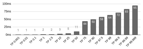
Figure 3-7. Node.js gzip compression latency
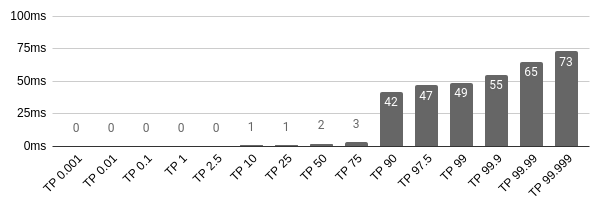
Figure 3-8. HAProxy gzip compression latency
This test shows that requests are served quite a bit quicker using HAProxy for performing gzip compression than when using Node.js.
TLS Termination
TLS absolutely has a negative impact on application performance (in an HTTP versus HTTPS sense). These tests just compare the performance impact of performing TLS termination within HAProxy instead of Node.js, not HTTP compared to HTTPS. The throughput numbers have been reproduced below since the tests run so fast that the latency listing graphs mostly contains zeros.
First, performing TLS Termination within the Node.js process is tested. For this test use the same recipe-api/producer-https-basic.js file that created in Example 2-7, commenting out any console.log statements from the request handler:
$ PORT=3001node recipe-api/producer-https-basic.js$haproxy -f haproxy/passthru.cfg$autocannon -d60-c10https://localhost:3000/recipes/42
Table 3-9 contains the results of running this load-test on my machine.
| Stat | 1% | 2.5% | 50% | 97.5% | Avg | Stdev | Min |
|---|---|---|---|---|---|---|---|
Req/Sec |
10215 |
14511 |
17903 |
19167 |
17728.41 |
1344.34 |
10212 |
Bytes/Sec |
3.62 MB |
5.14 MB |
6.34 MB |
6.79 MB |
6.28 MB |
476 kB |
3.62 MB |
Next, to test HAProxy, make use of the recipe-api/producer-http-basic.js file created back in Example 1-5 (again, comment out the console.log calls), as well as the haproxy/tls.cfg file from Example 3-8:
$ PORT=3001node recipe-api/producer-http-basic.js$haproxy -f haproxy/tls.cfg$autocannon -d60-c10https://localhost:3000/recipes/42
Table 3-10 contains the results of running this load-test on my machine.
| Stat | 1% | 2.5% | 50% | 97.5% | Avg | Stdev | Min |
|---|---|---|---|---|---|---|---|
Req/Sec |
9647 |
12631 |
16927 |
18623 |
16575.14 |
1435.03 |
9642 |
Bytes/Sec |
3.18 MB |
4.17 MB |
5.59 MB |
6.14 MB |
5.47 MB |
473 kB |
3.18 MB |
In this case, a drop of a few percent is seen when having HAProxy perform the TLS Termination instead of Node.js! However, take this with a grain of salt. The JSON payload being used so far is about 200 bytes long. With a larger payload, for example 150kb, HAProxy will usually outperform Node.js when doing TLS Termination.
As with all benchmarks, it’s important to test your application in your environment. The services used in this book are quite simple; a “real” application, doing CPU intensive work like template rendering, and sending documents with varying payload sizes, will behave completely different.
Protocol Concerns
Now you’ll load test some of the previously covered protocols, namely JSON over HTTP, GraphQL, and gRPC. Since these approaches do change the payload contents, measuring their transmission over a network will be more important than in “Reverse Proxy Concerns”. Also, recall that protocols like gRPC are more likely to be used for cross-service traffic than for external traffic. For that reason I’ll run these load tests on two different machines within the same cloud provider data center.
For these tests your approach is going to cheat a little bit. Ideally, you’d build a client from scratch, one that would natively speak the protocol being tested and would measure the throughput. But, since you already built the web-api clients that accept HTTP requests, you’ll simply point Autocannon at those so you don’t need to build three new applications. This is visualized in Figure 3-9.

Figure 3-9. Benchmarking in the cloud
Since there’s an additional network hop this approach can’t accurately measure performance, like X is Y% faster than Z, but it can rank their performance—as implemented in Node.js using these particular libraries—from fastest to slowest.
If you have access to a cloud provider and a few dollars to spare, feel free to spin up two new VPS instances and copy the examples/ directory that you have so far to them. You should use machines with at least two CPU cores. This is particularly important on the client where Autocannon and web-api might compete for CPU access with a single core. Otherwise, you can also run the examples on your development machine, at which point you can omit the TARGET environment variable.
Be sure to substitute <RECIPE_API_IP> for the IP address or hostname of the recipe-api service in each of the following examples.
JSON over HTTP
This first load test will benchmark the recipe-api/producer-http-basic.js service created in Example 1-5 by sending requests through the web-api/consumer-http-basic.js service created in Example 1-6:
# Server VPS$ HOST=0.0.0.0 node recipe-api/producer-http-basic.js# Client VPS$ TARGET=<RECIPE_API_IP>:4000 node web-api/consumer-http-basic.js$autocannon -d60-c10-l http://localhost:3000
My results for this benchmark appear in Figure 3-10.

Figure 3-10. Benchmarking JSON over HTTP
GraphQL
This next load test will use the recipe-api/producer-graphql.js service created in Example 2-11 by sending requests through the web-api/consumer-graphql.js service created in Example 2-12:
# Server VPS$ HOST=0.0.0.0 node recipe-api/producer-graphql.js# Client VPS$ TARGET=<RECIPE_API_IP>:4000 node web-api/consumer-graphql.js$autocannon -d60-c10-l http://localhost:3000
My results for this load test appear in Figure 3-11.
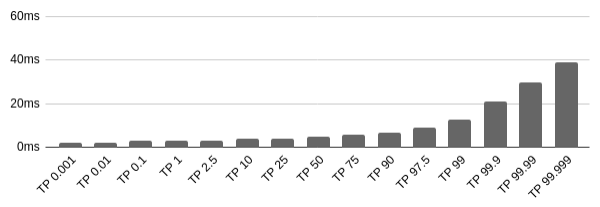
Figure 3-11. Benchmarking GraphQL
gRPC
This final load test will test the recipe-api/producer-grpc.js service created in Example 2-14 by sending requests through the web-api/consumer-grpc.js service created in Example 2-15:
# Server VPS$ HOST=0.0.0.0 node recipe-api/producer-grpc.js# Client VPS$ TARGET=<RECIPE_API_IP>:4000 node web-api/consumer-grpc.js$autocannon -d60-c10-l http://localhost:3000
My results for this load test appear in Figure 3-12.
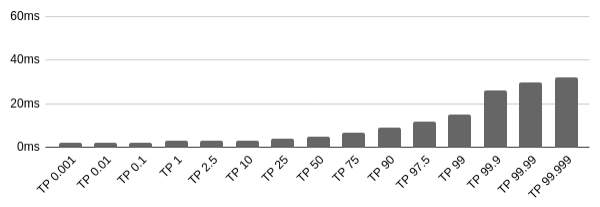
Figure 3-12. Benchmarking gRPC
Conclusion
According to these results, JSON over HTTP is typically the fastest, with GraphQL being the second fastest, and gRPC being the third fastest. Interestingly, the most extreme cases follow the opposite pattern, with the worst case gRPC case being faster than GraphQL, and GraphQL being faster than JSON over HTTP.
The reason for this is that JSON.stringify() is extremely optimized in V8, so any other serializer is going to have a hard time keeping up. GraphQL has its own parser for parsing the query strings, which will add some additional latency versus a query represented purely using JSON. gRPC needs to switch contexts between JavaScript and C++ to do parsing and serializing. This means gRPC should be faster in more static, compiled languages like C++ than in JavaScript.
Formulating an SLA
An SLA can cover many different aspects of a service. Some of these are business-related requirements, like the service will not ever double charge a customer for a single purchase. Others are the topic of this section, like the service will have a TP99 latency of 200ms and will have an uptime of 99.9%.
Coming up with an SLA for latency can be tricky. For one thing, the time it will take for your application to serve a response will depend on the time it takes an upstream service to return its response. If you’re adopting the concept of an SLA for the first time, you’ll need upstream services to also come up with an SLA of their own. Otherwise, when their service latency jumps from 20ms to 40ms, who’s to know if they’re actually doing something wrong?
Another thing to keep in mind is that your service will very likely receive more traffic during certain times of the day and certain days of the week, especially if traffic is governed by the interactions of people. For example, a backend service used by an online retailer will get more traffic on Mondays, in the evenings, and near holidays, whereas a service receiving periodic sensor data will always handle data at the same rate. Whatever SLA you do decide on will need to hold true during times of peak traffic.
Something that can make measuring performance difficult is the concept of the Noisy Neighbor. This is a problem that occurs when a service is running on a machine with other services, those other services end up consuming too many resources, such as CPU or bandwidth. This can cause your service to take more time to respond.
When first starting with an SLA, it’s useful to perform a load test on your service as a starting point. For example, Figure 3-13 is the result of benchmarking a production application that I built. With this service the TP99 has a latency of 57ms. To get it any faster would require performance work.

Figure 3-13. Benchmarking a production application
Be sure to completely mimic production situations when load testing your service. For example, if a real consumer will make a request through a reverse proxy, then make sure your load tests also go through the same reverse proxy, instead of connecting directly to the service.
Another thing to consider is what the consumers of your service are expecting. For example, if your service provides suggestions for an autocomplete form when a user types a query, having a response time less than 100ms is vital. On the other hand, if your service triggers the creation of a bank loan, having a response time of 60s might also be acceptable.
If an downstream service has a hard response time requirement, and you’re not currently satisfying it, you’ll have to find a way to make your service more performant. You can try throwing more servers at the problem, but often times, you’ll need to get into the code and make things faster. Consider adding a performance tests when code is being considered for merging (“Automated Testing” discusses automated tests in further detail).
When you do determine a latency SLA, you’ll then want to determine how many service instances to run. For example, you might have an SLA where the TP99 response time is 100ms. Perhaps a single server is able to perform at this level when handling 500 requests per minute. However, when the traffic increases to 1,000 requests per minute, the TP99 drops to 150ms. In this situation you’ll need to add a second service. Experiment with adding more services, and testing load at different rates, to understand how many services it takes to double, triple, or even 10x your traffic.
Autocannon has the -R flag for specifying an exact number of requests per second. Use this to throw an exact rate of requests at your service. Once you do that, you can measure your application at different request rates and find out where it stops performing at the intended SLA. Once that happens, add another service instance, and test again. Using this method, you’ll know how many service instances are needed in order to satisfy the TP99 SLA based on different overall throughputs.
Using the cluster-fibonacci.js application created in Example 3-2 as a guide, you’ll now attempt to measure just this. This application, with a Fibonacci limit of 10,000, is an attempt to simulate a real service. The TP99 value you’ll want to maintain is 20ms. Create another HAProxy configuration file haproxy/fibonacci.cfg based on the content in Example 3-14. You’ll iterate on this file as you add new service instances.
Example 3-14. haproxy/fibonacci.cfg
defaults
  mode http

frontend inbound
  bind localhost:5000
  default_backend fibonacci

backend fibonacci
  server fibonacci-1 localhost:5001
# server fibonacci-2 localhost:5002
# server fibonacci-3 localhost:5003
This application is a little too CPU heavy. Add a sleep statement to simulate a slow database connection, which should keep the event loop a little busier. To make this change, introduce a sleep() function like this one, causing requests to take at least 10ms longer than usual:
// Add this line inside the server.get async handlerawaitsleep(10);// Add this function to the end of the filefunctionsleep(ms){returnnewPromise(resolve=>setTimeout(resolve,ms));}
Next, run a single instance of cluster-fibonacci.js, as well as HAProxy, using the following commands:
$ PORT=5001node cluster-fibonacci.js# later run with 5002 & 5003$haproxy -f haproxy/fibonacci.cfg$autocannon -d60-c10-R10http://localhost:5000/10000
My TP99 value is 18ms, which is below the 20ms SLA, so I know that one instance can handle traffic of at least 10 r/s. So, now double that value! Run the Autocannon command again by setting the -R flag to 20. On my machine the value is now 24ms, which is too high. Of course, your results will be different. Keep tweaking the requests per second value until you reach the 20ms TP99 SLA threshold. At this point you’ve discovered how many requests per second a single instance of your service can handle! Write that number down.
Next, uncomment the second to last line of the haproxy/fibonacci.cfg file. Also, run another instance of cluster-fibonacci.js, setting the PORT value to 5002. Restart HAProxy to reload the modified config file. Then, run the Autocannon command again, with increased traffic. Increase the requests per second until you reach the threshold again, and write down the value. Do it a third and final time. Table 3-11 contains my results.
Instance Count |
1 |
2 |
3 |
Max r/s |
12 |
23 |
32 |
With this information I can deduce that if my service needs to run with 10 requests per second, then a single instance will allow me to honor my 20ms SLA for my consumers. If, however, the holiday season is coming, and I know consumers are going to want to calculate the 5000th Fibonacci sequence at a rate of 25 requests per second, then I’m going to need to run three instances.
If you work in an organization that doesn’t currently make any performance promises, I encourage you to measure your service’s performance and come up with an SLA using current performance as a starting point. Add that SLA to your project’s README document and strive to improve it each quarter.