Chapter 4. Observability
This chapter is dedicated to observing the state of a Node.js service running on a remote machine. Locally, tools like the debugger or console.log() make this easy. But, once a service is running in a far away land, you’ll need to reach for a different set of tools.
When debugging locally, you’re usually concerned about a single request. You ask yourself, “When I pass this value into a request, why do I get that value in the response?” By logging the inner workings of a function, you gain insight into why a function behaved in an unanticipated way. This chapter looks at technologies useful for debugging an individual request as well. “Logging with ELK” looks at log generation, which is a way to keep track of very verbose information on a per-instance basis, much like you might print with console.log(). Later, “Distributed Request Tracing with Zipkin” looks at a tool for tracking upstream sub-requests, no matter which service generates the log.
You often need to gain insight into things that wouldn’t normally be considered a hard bug when dealing with production traffic. For example, you might have to ask, “Why are HTTP requests 100ms slower for users created before April 2020?” This information might not be noticeable when making a single request. However, when such metrics are viewed in aggregate over many request, you’re then able to spot trends. “Metrics with Graphite, StatsD, and Grafana” covers this in more detail.
In a related concept, you’ll also build functionality into an application so that it can determine whether or not its healthy in “Health Checks”. With this information, a service can declare itself unfit to serve requests.
These tools mostly display information passively in a dashboard of some sort, which an engineer can later look at and determine the source of a problem. “Alerting with Cabot” covers how to send a warning to a developer when an application’s performance dips below a certain threshold, thus allowing them to prevent an issue before it happens.
Environments
Environments are a concept for differentiating running instances of an application, as well as databases, from each other. They’re important for various reasons, including choosing which instances to route traffic to, keeping metrics and logs separate (which is particularly important in this chapter), segregating services for security, and for gaining confidence that a checkout of application code is going to be stable in one environment before it is deployed to production.
Environments should remain segregated from one another. If you control your own hardware, this could mean running different environments on different physical servers. If you’re deploying your application to the cloud, this more likely means setting up different VPCs (Virtual Private Clouds)—a concept supported by both AWS and GCP.
At an absolute minimum, any application will need at least a single production environment. This is the environment responsible for handling requests made by public users. However, you’re going to want a few more environments than that, especially as your application grows in complexity.
As a convention, Node.js applications generally use the NODE_ENV environment variable to specify which environment an instance is running in. This value can be set in different ways. For testing it can be set manually, like with the following example, but for production use, whatever tool you use for deploying will abstract this process away:
$exportNODE_ENV=production$node server.js
Philosophies for choosing what code to deploy to different environments, branching and merging strategies, and even which VCS (version control system) to choose is outside the scope of this book. But, ultimately, a particular snapshot of the codebase is chosen to be deployed to a particular environment.
Choosing which environments to support is also important, and also outside of the scope of this book. Usually companies will have, at a minimum, the following environments:
- Development
-
Used for local development. Perhaps other services know to ignore messages associated with this environment. Doesn’t need some of the backing stores required by production, for example, logs might be written to stdout instead of being transmitted to a collector.
- Staging
-
Represents an exact copy of the production environment, such as machine specs and operating system versions. Perhaps an anonymized database snapshot from production is copied to a staging database via a nightly cron job.
- Production
-
Where the real, production traffic is processed. There may be more service instances here than in preprod; for example, maybe preprod runs two application instances (always run more than one) but production runs eight.
The environment string must remain consistent across all applications, both those written using Node.js and those on other platforms. This consistency will prevent many headaches. If one team refers to an environment as staging and the other as preprod, querying logs for related messages then becomes an error-prone process.
The environment value shouldn’t necessarily be used for configuration—for example, having a lookup map where environment name is associated with a hostname for a database. Ideally, any dynamic configuration should be provided via environment variables. Instead, the environment value is mostly used for things related to observability. For example, log messages should have the environment attached in order to help associate any logs with the given environment, which is especially important if a logging service does get shared across environments. [Link to Come] takes a deeper look at configuration.
Logging with ELK
ELK, or more specifically, The ELK Stack, is a reference to Elasticsearch, Logstash, and Kibana, three open source tools built by Elastic. When combined, these powerful tools are often the platform of choice for performing on-prem logging. Individually, each of these tools serves a different purpose:
- Elasticsearch
-
A database with a powerful query syntax, supporting features like natural text searching. It is useful for many more situations than what are covered in this book, and is worth considering if you ever need to build a search engine. It exposes an HTTP API and has a default port of
:9200. - Logstash
-
A service for ingesting and transforming logs from multiple sources. You’ll create an interface so that it can ingest logs via UDP. It doesn’t have a default port so we’ll just use
:7777. - Kibana
-
A web service for building dashboards that visualize data stored in Elasticsearch. It exposes an HTTP web service over the port
:5601.
Figure 4-1 diagrams these services and their relationships, as well as how they’re encapsulated using Docker in the upcoming examples.
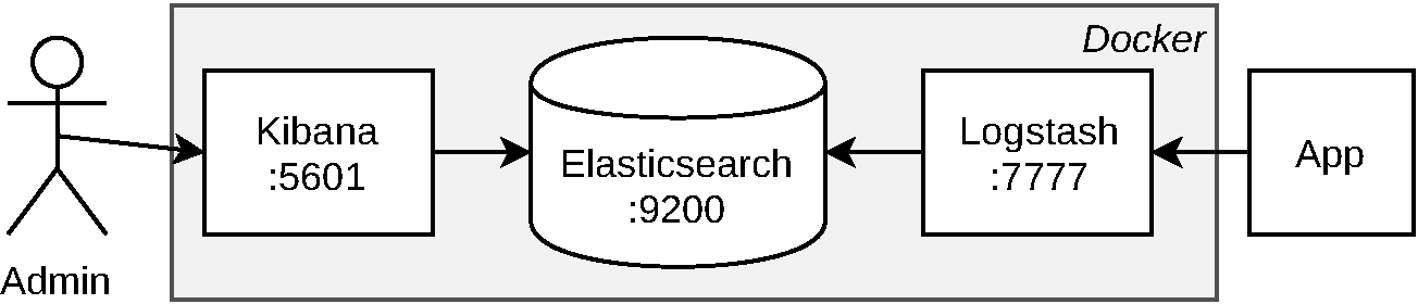
Figure 4-1. The ELK stack
Your application is expected to transmit well-formed JSON logs, typically an object that’s one or two levels deep. These objects contain generic metadata about the message being logged, such as timestamp and host and IP address, as well as information specific to the message itself, such as level/severity, environment, and a human-readable message. There are multiple ways to configure ELK to receive such messages, such as writing logs to a file and using Elastic’s Filebeat tool to collect them. The approach used in this section will configure Logstash to listen for incoming UDP messages.
Running ELK via Docker
In order to get your hands dirty, you’re going to run a single Docker container containing all three services (be sure to have Docker installed—see [Link to Come] for more information). These examples won’t enable disk persistence. Within a larger organization, each of these services would perform better when installed on dedicated machines, and of course, persistence is vital.
In order to configure Logstash to listen for UDP messages a configuration file must first be created. The content for this file is available in Example 4-1 and can be placed in a new directory at misc/elk/udp.conf. Once the file is created, you’ll make it available to the Logstash service running inside of the Docker container. This is done by using the -v volume flag, allowing a local filesystem path to be mounted inside of the container’s filesystem.
Example 4-1. misc/elk/udp.conf
input {
  udp {
    id => "nodejs_udp_logs"
    port => 7777
    codec => json
  }
}
output {
  elasticsearch {
    hosts => ["localhost:9200"]
    document_type => "nodelog"
    manage_template => false
    index => "nodejs-%{+YYYY.MM.dd}"
  }
}
Note
For brevity’s sake, these examples use UDP for sending messages. This approach doesn’t come with the same delivery guarantees as others, such as delivery guarantees or back pressure support, but it does come with reduced overhead for the application. Be sure to research the best tool for your use-case.
Once the file has been created you’re ready to run the container using the commands in Example 4-2. If you’re running Docker on a Linux machine, you’ll need to run the sysctl command before the container will properly run, and you may omit the -e flag if you want. Otherwise, if you’re running Docker on a macOS machine, skip the sysctl flag.
Example 4-2. Running ELK within Docker
$sudo sysctl -w vm.max_map_count=262144# Linux Only$docker run -p 5601:5601 -p 9200:9200-p 5044:5044 -p 7777:7777/udp-v$PWD/misc/elk/udp.conf:/etc/logstash/conf.d/99-input-udp.conf-eMAX_MAP_COUNT=262144-it --name distnode-elk sebp/elk:683
This command downloads files from Dockerhub and configures the service and may take a few minutes to run. Once your console calms down a bit, visit http://localhost:5601 in your browser. If you see a successful message then the service is now ready to receive messages.
Transmitting Logs from Node.js
For this example, you’re going to again start by modifying an existing application. Copy the web-api/consumer-http-basic.js file created in Example 1-6 to web-api/consumer-http-logs.js as a starting point. Next, modify the file to look like the code in Example 4-3 (note that the first several lines are the same and have been truncated from the code example).
Example 4-3. web-api/consumer-http-logs.js (truncated)
constlog=require('./logstash.js');server.use((req,res,next)=>{log('info','request-incoming',{path:req.url,method:req.method,ip:req.ip,ua:req.headers['user-agent']||null});next();});server.setErrorHandler(async(error,req)=>{log('error','request-failure',{stack:error.stack,path:req.url,method:req.method,});return{error:error.message};});server.get('/',async()=>{consturl=`http://${TARGET}/recipes/42`;log('info','request-outgoing',{url,svc:'recipe-api'});constreq=awaitfetch(url);constproducer_data=awaitreq.json();return{consumer_pid:process.pid,producer_data};});server.get('/error',async()=>{thrownewError('oh no');});server.listen(PORT,HOST,()=>{log('verbose','listen',{host:HOST,port:PORT});});

The new logstash.js file is now being loaded.

A middleware to log incoming requests.

A call to the logger that passes in request data.

A generic middleware for logging errors.

Information about outbound requests are logged.

Information about server starts are also logged.
This file logs some key pieces of information. The first thing logged is when the server starts. The second set of information is by way of a generic middleware handler. It logs data about any incoming request, including the path, the method, the IP address, and the user agent. This is similar to the access log for a traditional web server. And finally, the application tracks outbound requests to the recipe-api service.
The contents of the logstash.js file might be more interesting. There are many libraries available on npm for transmitting logs to Logstash (@log4js-node/logstashudp is one such module). These libraries support a few methods for transmission, UDP included. Since the mechanism for sending logs is so simple you’re going to reproduce a version from scratch. This is great for educational purposes, but a full-featured module from npm will make a better choice for a production application.
Create a new file called web-api/logstash.js. Unlike the other JavaScript files you’ve created so far, this one won’t be executed directly. Add the content from Example 4-4 to this file.
Example 4-4. web-api/logstash.js
constclient=require('dgram').createSocket('udp4');consthost=require('os').hostname();const[LS_HOST,LS_PORT]=process.env.LOGSTASH.split(':');constNODE_ENV=process.env.NODE_ENV;module.exports=function(severity,type,fields){constpayload=JSON.stringify({'@timestamp':(newDate()).toISOString(),"@version":1,app:'web-api',environment:NODE_ENV,severity,type,fields,host});console.log(payload);client.send(payload,LS_PORT,LS_HOST);};
The built-in dgram module sends UDP messages.
The Logstash location is stored in
LOGSTASH.Several fields are sent in the log message.
This basic Logstash module exports a function that application code calls to send a log. Many of the fields are automatically generated, like @timestamp, which represents the current time. The app field is the name of the running application, and doesn’t need to be overridden by the caller. Other fields, like severity and type, are fields that the application is going to change all the time. The fields field represents additional key/value pairs the app might want to provide.
The severity field refers to the log severity. Most logging modules support the following six values, originally made popular by the npm client: error, warn, info, verbose, debug, silly. It’s a common pattern with more “complete” logging modules to set a logging threshold via environment variable. For example, by setting the minimum severity to verbose, any messages with a lower severity (namely debug and silly), will get dropped. The overly simple logstash.js module doesn’t support this.
Once the payload has been constructed it’s then converted into a JSON string, printed to the console to help tell what’s going on, and finally, the process attempts to transmit the message to the Logstash server (there is no way for the application to know if the message was delivered; thus is the shortcoming of UDP).
With the two files created it’s now time to test the application. Run the commands in Example 4-5. This will start an instance of the new web-api service, an instance of the previous recipe-api service, and will also send a series of requests to the web-api. A log will be immediately sent once the web-api has been started, and two additional logs will be sent for each incoming HTTP request. Note that the watch commands continuously execute the command following on the same line and will need to be run in separate terminal windows.
Example 4-5. Running web-api and generating logs
$ NODE_ENV=developmentLOGSTASH=localhost:7777node web-api/consumer-http-logs.js$node recipe-api/producer-http-basic.js$brew install watch# required for macOS$watch -n5 curl http://localhost:3000$watch -n13 curl http://localhost:3000/error
Isn’t that exciting? Well, not quite yet. Now you’ll jump into Kibana and take a look at the logs being sent. Let the watch commands continue running in the background; they’ll keep the data fresh while you’re using Kibana.
Creating a Kibana Dashboard
Now that the application is sending data to Logstash, and Logstash is storing the data in Elasticsearch, it’s time to open Kibana and explore this data. Open your browser and visit localhost:5601. At this point you should be greeted with the Kibana dashboard.
Within the dashboard, click the last tab on the left, entitled Management. Next, locate the Kibana section of options then click the Index Patterns option. Click Create index pattern. For Step 1, type in an Index pattern of nodejs-*. You should see a small Success! message below as Kibana correlates your query to a result. Click Next step. For Step 2, click the Time Filter drop-down, then click the @timestamp field. Finally, click Create index pattern. You’ve now created an index named nodejs-* that will allow you to query those values.
Click the second tab on the left, titled Visualize. Next, click the Create new visualization button in the center of the screen. You’ll be given several different options for creating a visualization, including the ones shown in Figure 4-2, but for now just click the Vertical Bar graph option.
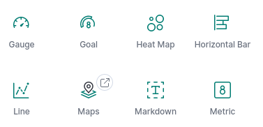
Figure 4-2. Kibana visualizations
Select the nodejs-* index that you just created. Once that’s done you’ll be taken to a new screen to fine tune the visualization. The default graph isn’t too interesting; it’s a single bar showing a count of all logs matching the nodejs-* index. But not for long.
The goal now is to create a graph that displays the rate at which incoming requests are received by the web-api service. So, first add a few filters to narrow down the results to only contain applicable entries. Click the + Add Filter link near the upper left corner of the screen. For the Field drop-down, enter the value type. For the Operator field, set it to is. For the Value field, enter the value request-incoming. Next, click + Add Filter again, and do the same thing, but this time set Field to app, then set Operator to is again, and set Value to web-api.
For the Metrics section, leave it displaying the count, since it should display the number of requests and the matching log messages correlate one to one with real requests.
For the Buckets section, it should be changed to group by time. Click the + Add link, and select X-Axis. For the Aggregation drop-down, select Date Histogram. With your cursor still in the field, press Enter, and the graph will update. The default settings of grouping by @timestamp with an automatic interval is fine.
In the upper-right corner is a drop-down for changing the time range of the logs being queried. Click the drop-down and configure it to display logs from the last one hour, then click the large Update button to the right of the drop-down. If all goes to plan, your screen should look like Figure 4-3.
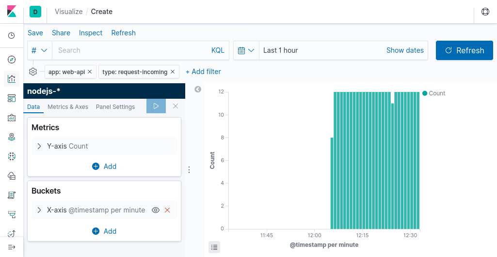
Figure 4-3. Requests over time in Kibana
Once your graph is complete, click the Save link in the upper right corner of the Kibana page. Name the visualization as web-api incoming requests. Next, create a similar visualization, but this time set the type field to request-outgoing, and name that visualization as web-api outgoing requests, and finally create a third visualization with a type field of listen and name it as web-api server starts.
Next, you’ll create a dashboard for these three visualizations. Select the third option in the sidebar titled Dashboard. Then, click the Add link at the top of the screen. A modal window will appear with your three visualizations in it. Click each visualization and they will be added to the dashboard. Once you’ve added each visualization, dismiss the modal. Click the Save link at the top of the screen and save the dashboard as web-api overview.
Congratulations! You’ve created a dashboard containing information extracted from your application.
Running Ad-Hoc Queries
Sometimes you’ll need to run arbitrary queries against the data that’s being logged without a correlating dashboard. This is helpful in one-off debugging situations. In this section you’ll write arbitrary queries in order to extract errors about the application.
Click the first tab in the left sidebar, the one titled Discover. This is a convenient playground for running queries without needing to commit them to a dashboard. By default, a listing of all recently received messages is displayed. Click inside of the Search field at the top of the screen. Then, type the following query into the search field and press Enter:
app:"web-api" AND (severity:"error" OR severity:"warn")
The syntax of this query is written in the Kibana Query Language (KQL). Essentially, there are three clauses. It’s asking for logs belonging to the web-api application, and whose severity levels are set to either error or warn (in other words, things that are very important).
Click the arrow symbol next to one of the log entries in the list that follows. This will expand the individual log entry and allow you to view the entire JSON payload associated with the log. The ability to view arbitrary log messages like this is what makes logging so powerful. With this tool you’re now able to find all the errors being logged from the service.
By logging more data, you’ll gain the ability to drill down into the details of specific error situations. For example, you might find that errors occur when a specific endpoint within an application is being hit, under certain circumstances (like a user updating a recipe via PUT /recipe in a more full featured application). With access to the stack trace, and enough contextual information about the requests, you’re then able to recreate the conditions locally, reproduce the bug, and come up with a fix.
Warning
This section looks at transmitting logs from within an application, an inherently asynchronous operation. Unfortunately, logs generated when a process crashes might not be sent in time. Many deployment tools can read messages from stdout and transmit them on behalf of the application, which increases the likelihood of them being delivered.
This section looked at storing logs. Certainly, these logs can be used to display numeric information in graphs, but it isn’t necessarily the most efficient system for doing so since it stores complex objects. The next section, “Metrics with Graphite, StatsD, and Grafana”, looks at storing more interesting numeric data using a different set of tools.
Metrics with Graphite, StatsD, and Grafana
“Logging with ELK” looked at transmitting logs from a running Node.js process. Such logs are formatted as JSON, and are indexable and searchable on a per-log basis. This is perfect for reading messages related to a particular running process, such as reading variables and stack traces. However, sometimes you don’t necessarily care about individual pieces of numeric data, and instead you want to know about aggregations of data, usually as these values grow and shrink over time.
This section looks at sending metrics. A metric is numeric data associated with time. This can include things like request rates, the number of 2XX versus 5XX HTTP responses, latency between the application and a backing service, memory and disk use, and even business stats like dollar revenue or cancelled payments. Visualizing such information is important to understanding application health and system load.
Much like in the logging section, a stack of tools will be used instead of a single one. However, this stack doesn’t really have a catchy acronym like ELK, and it’s fairly common to swap out different components. The stack considered here is that of Graphite, StatsD, and Grafana.
- Graphite
-
A combination of a service (Carbon), and time series database (Whisper). It also comes with a UI (Graphite Web), though the more powerful Grafana interface is often used.
- StatsD
-
A daemon (built with Node.js) for collecting metrics. It can listen for stats over TCP or UDP before sending aggregations to a backend such as Graphite.
- Grafana
-
A web service that queries time series backends (like Graphite) and displays information in configurable dashboards.
Figure 4-4 shows a diagram of these services and how they’re related. The Docker boundaries represent what the upcoming examples will use.
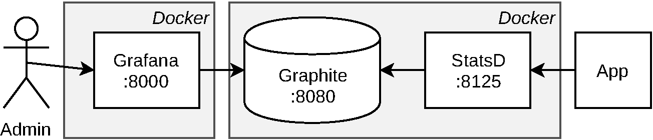
Figure 4-4. Graphite, StatsD, and Grafana
Much like in the logging section, these examples will transmit data using UDP. Due to the nature of metrics being rapidly produced, using UDP will help keep the application from getting overwhelmed.
Running via Docker
Example 4-6 starts two separate Docker containers. The first one, graphiteapp/graphite-statsd contains StatsD and Graphite. Two ports from this container are exposed. The Graphite UI / API is exposed via port :8080, while the StatsD UDP metrics collector is exposed as :8125. The second, grafana/grafana, contains Grafana. A single port for the web interface, :8000, is exposed for this container.
Example 4-6. Running StatsD + Graphite, and Grafana
$docker run-p 8080:80-p 8125:8125/udp-it --name distnode-graphite graphiteapp/graphite-statsd:1.1.6-1$docker run-p 8000:3000-it --name distnode-grafana grafana/grafana:6.5.2
Once the containers are up and running, open a web browser and visit the Grafana dashboard at localhost:8000. You’ll be asked to login at this point. The default login credentials are admin / admin. Once you successfully log-in, you’ll then be prompted to change the password to something else. This password will be used to administer Grafana, though it won’t be used in code.
Once the password has been set, you’ll be taken to a wizard for configuring Grafana. The next step is to configure Grafana to communicate with the Graphite image. Click the Add Data Source button, then click the Graphite option. On the Graphite configuration screen, input the values displayed in Table 4-1.
Name |
Dist Node Graphite |
URL |
http://<LOCAL_IP>:8080 |
Version |
1.1.x |
Note
Due to the way these Docker containers are being run, you won’t be able to use localhost for the <LOCAL_IP> placeholder. Instead, you’ll need to use your local IP address. If you’re on Linux, try running hostname -I, and if you’re on macOS, try running ipconfig getifaddr en0. If you’re running this on a laptop, and your IP address changes, you’ll need to reconfigure the data source in Grafana to use the new IP address, otherwise you won’t get data.
Once you’ve entered the data, click Save & Test. If you see the message Data source is working, then Grafana was able to talk to Graphite and you can click the Back button. If you get HTTP Error Bad Gateway, make sure the Graphite container is running and that the settings have been entered correctly.
Now that Graphite and Grafana are talking to each other, it’s time to modify one of the Node.js services to start sending metrics.
Transmitting Metrics from Node.js
The protocol used by StatsD is extremely simple, arguably even simpler than the one used by Logstash UDP. An example message which increments a metric named foo.bar.baz looks like this:
foo.bar.baz:1|c
Such interactions could very easily be rebuilt using the dgram module like in the previous section. However, this code sample will make use of an existing module. There are a few out there but this example uses the statsd-client module.
Again, start by rebuilding a version of the consumer service. Copy the web-api/consumer-http-basic.js file created in Example 1-6 to web-api/consumer-http-metrics.js as a starting point. From there, modify the file to resemble Example 4-7. Be sure to run the npm install command to get the required module as well.
Example 4-7. web-api/consumer-http-metrics.js (first-half)
#!/usr/bin/env node// npm install fastify@2 node-fetch@2 [email protected]constserver=require('fastify')();constfetch=require('node-fetch');constHOST='127.0.0.1';constPORT=process.env.PORT||3000;constTARGET=process.env.TARGET||'localhost:4000';constSDC=require('statsd-client');conststatsd=new(require('statsd-client'))({host:'localhost',port:8125,prefix:'web-api'});server.use(statsd.helpers.getExpressMiddleware('inbound',{timeByUrl:true}));server.get('/',async()=>{constbegin=newDate();constreq=awaitfetch(`http://${TARGET}/recipes/42`);statsd.timing('outbound.recipe-api.request-time',begin);statsd.increment('outbound.recipe-api.request-count');constproducer_data=awaitreq.json();return{consumer_pid:process.pid,producer_data};});server.get('/error',async()=>{thrownewError('oh no');});server.listen(PORT,HOST,()=>{console.log(`Consumer running at http://${HOST}:${PORT}/`);});
Metric names are prefixed with
web-api.A generic middleware that automatically tracks inbound requests.
This tracks the perceived timing to recipe-api.
The number of outbound requests is also tracked.
A few things are going on with this new set of changes. First, it requires the statsd-client module, and configures a connection to the StatsD service listening at localhost:8125. It also configures the module to use a prefix value of web-api. This value represents the name of the service reporting the metrics (likewise, if you made similar changes to recipe_api, you’d set its prefix accordingly). Graphite works by using a hierarchy for naming metrics, and so, metrics sent from this service will all have the same prefix to differentiate them from metrics sent by another service.
The code makes use of a generic middleware provided by the statsd-client module. As the method name implies, it was originally designed for Express, but Fastify mostly supports the same middleware interface, so this application is able to reuse it. The first argument is another prefix name, and inbound implies that the metrics being sent here are associated with incoming requests.
Next, two values are manually tracked. The first is the amount of time the web-api perceives the recipe-api to have taken. Note that this time should always be longer than the time recipe_api believes the response took. This is due to the overhead of sending a request over the network. This timing value is written to a metric named outbound.recipe-api.request-time. The application also tracks how many requests are sent. This value is provided as outbound.recipe-api.request-count. You could even get more granular here. For example, for a production application, the status codes that the recipe-api responds with could also be tracked, which would allow an increased rate of failures to be visible.
Next, run the commands in Example 4-8 each in a separate terminal window. This will start your newly created service, run a copy of the producer, run Autocannon to get a stream of good requests, and also trigger some bad requests.
Example 4-8.
$ NODE_DEBUG=statsd-client node web-api/consumer-http-metrics.js$node recipe-api/producer-http-basic.js$autocannon -d300-R5-c1http://localhost:3000$watch -n1 curl http://localhost:3000/error
Those commands will generate a stream of data, which gets passed to StatsD before being sent to Graphite. Now that you have some data, you’re ready to create a dashboard to view it.
Creating a Grafana Dashboard
As the owner of the web-api service, there are (at least) three different sets of metrics that should be extracted so that you can measure its health. This includes the incoming requests, and importantly, differentiating 200’s from 500’s. It also includes the amount of time that recipe-api, an upstream service, takes to reply. The final set of required information is the rate of requests to the recipe-api service. If you determine the web-api service is slow, you might use this information to discover that the recipe-api service is slowing it down.
Switch back to your web browser with the Grafana interface. There is a large plus symbol in the sidebar; click it to be taken to the New dashboard screen. On this screen you’ll see a New Panel rectangle. Inside of it is an Add Query button. Click that button to be taken to the query editor screen.
On this new screen you’ll see an empty graph at the top, and inputs to describe the graph below. The UI lets you describe the query using two fields. The first is called Series, and is where you can input in the hierarchical metric name. The second field is called Functions. Both of these fields provide autocomplete for matching metric names. First start with the Series field. Click the select metric text next to the Series label, then click stats_count from the drop down. Then click select metric again, and select web-api. Continue this for the values inbound, response_code, and finally * (the * is a wildcard and will match any value). At this point the graph has been updated and should show two sets of entries.
The graph labels aren’t too friendly just yet. They’re displaying the entire hierarchy name, instead of just the easy-to-read values 200 and 500. A Function can be used to fix this. Click the plus sign next to the Functions label, then click Alias, then click aliasByNode(). This will insert the function, and also automatically provide a default argument of 4. This is because the asterisk in the query is the 4th entry in the (zero based) hierarchy metric name. The graph labels have been updated to display just 200 and 500.
In the upper right corner of the panel with the Series and Functions fields, there’s a pencil icon with a tooltip titled Toggle text edit mode. Click that, and the graphical entry will change into a text version. This is helpful for quickly writing a query. The value you should have looks like the following:
aliasByNode(stats_counts.web-api.inbound.response_code.*, 4)
In the left column, click the gear icon labeled General. On this screen you’re able to modify generic settings about this particular graph. Click the Title field, and input a value of Incoming Status Codes. Once that’s done, click the large arrow in the upper left corner of the screen. This will take you from the panel editor screen and back to the dashboard edit screen. At this point, your dashboard will have a single panel.
Next, click the Add panel button in the upper right corner of the screen and then click the Add query button again. This will allow you to add a second panel to the dashboard. This next panel will track the time it takes to query the recipe-api. Create the appropriate Series and Functions entry to reproduce the following:
aliasByNode(stats.timers.web-api.outbound.*.request-time.upper_90, 4)
Note
StatsD is generating some of these metric names for you. For example, stats.timers is a StatsD prefix, web-api.outbound.recipe-api.request-time is provided by the application, and the timing-related metric names under that (such as upper_90) are again calculated by StatsD. In this case, the query is looking at TP90 timing values.
Since this graph measures time and is not a generic counter, the units should be modified as well (this information is measured in milliseconds). Click the second tab on the left, with a tooltip of Visualization. Then, scroll down the section labeled Axes, then find the group titled Left Y, then click the Unit drop down. Click Time, then click milliseconds (ms). The graph will then be updated with proper units.
Click the third General tab again, and set the panel’s title to Outbound Service Timing. Click the back arrow again to return to the dashboard edit screen.
Finally, click the Add panel button again, and go through creating a final panel. This panel will be titled Outbound Request Count, won’t need any special units, and will use the following query:
aliasByNode(stats_counts.web-api.outbound.*.request-count, 3)
Click the back button a final time to return to the dashboard editor screen. In the upper-right corner of the screen, click the Save dashboard icon, give the dashboard a name of Web API Overview, and save the dashboard. The dashboard is now saved and will have a URL associated with it. If you were using an instance of Grafana permanently installed for your organization, this URL would be a permalink that you could provide to others, and would make a great addition to your project’s README.
Feel free to drag the panels around and resize them until you get something that is aesthetically pleasing. In the upper right corner of the screen you can also change the time range. Set it to Last 15 minutes, since you likely don’t have data much older than that. Once your done, your dashboard should look something like Figure 4-5.
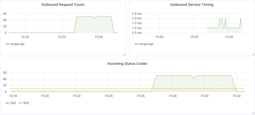
Figure 4-5. Completed Grafana dashboard
Node.js Health Indicators
There is some generic health information about a running Node.js process that is also worth collecting for the dashboard. Modify your web-api/consumer-http-metrics.js file by adding the code from Example 4-9 to the end of the file. Restart the service and keep an eye on the data that is being generated. These new metrics represent values that can increase or decrease over time, and are better represented as Gauges.
Example 4-9. Consumer service sending metrics to StatsD: web-api/consumer-http-metrics.js (second-half)
constv8=require('v8');constfs=require('fs');setInterval(()=>{statsd.gauge('server.conn',server.server._connections);constm=process.memoryUsage();statsd.gauge('server.memory.used',m.heapUsed);statsd.gauge('server.memory.total',m.heapTotal);consth=v8.getHeapStatistics();statsd.gauge('server.heap.size',h.used_heap_size);statsd.gauge('server.heap.limit',h.heap_size_limit);fs.readdir('/proc/self/fd',(err,list)=>{if(err)return;statsd.gauge('server.descriptors',list.length);});},10_000);
Number of connections to server.
Process heap utilization.
V8 heap utilization.
Open file descriptors.
This code will poll the Node.js underbelly every ten seconds for key information about the process. As an exercise of your newfound Grafana skills, create three new dashboards containing this newly-captured data. In the metric namespace hierarchy, they’ll begin with stats.gauges.
The first set of data, provided as server.conn, is the number of active connections to the web server. Most Node.js web frameworks expose this value in some manner, check out the documentation for your framework of choice.
Information about the process memory usage is also captured. These are being recorded as two values, server.memory.used and server.memory.total. When creating a graph for these values, their unit should be set to Data / Bytes, and Grafana is smart enough to display more specific units like MB. A very similar panel could then be made based on the V8 heap size and limit.
And finally, the number of open file descriptors can indicate a leak in a Node.js application. Sometimes files will get opened but will never get closed, and this can lead to consumption of server resources and result in a process crash.
Once you’ve added the new panels, your dashboard may then resemble Figure 4-6. Save the modified dashboard so that you don’t lose your changes.
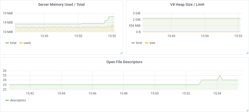
Figure 4-6. Updated Grafana dashboard
This section only covers the basics of what can be done with the StatsD, Graphite, and Grafana stack. There are many query functions that haven’t been covered, other forms of visualizations, individual time series entries can even be manually colored (like green for 2XX, yellow for 4XX, and red for 5XX), and so on.
Distributed Request Tracing with Zipkin
“Logging with ELK” looked at storing logs from a Node.js process. Such logs contain information about the internal operations of a process. Likewise, “Metrics with Graphite, StatsD, and Grafana” looked at storing numeric metrics. These metrics are useful for looking at numeric data in aggregate about an application, such as throughput and failure rates for an endpoint. However, neither of these tools allow for associating a specific external request with all the internal requests it may then generate.
Consider, for example, a slightly more complex version of the services covered so far. Instead of just a web-api and a recipe-api service, there’s an additional user-api and a user-store service. The web-api will still call the recipe-api service as before, but now the web-api will also call the user-api service, that will in turn call the user-store service. In this scenario, if any one of the services produces a 500 error, that error will bubble up and the overall request will fail with a 500. How would you find the cause of a specific error with the tools used so far?
Well, if you know that an error occurred on Tuesday at 1:37 P.M., you might be tempted to look through logs stored in ELK between the time of 1:36 P.M. and 1:38 P.M. Goodness knows I’ve done this myself. Unfortunately, if there is a high volume of logs, this could mean sifting through thousands of individual log entries. Worse, other errors happening at the same time can “muddy the water”, making it hard to know which logs are actually associated with the erroneous request.
At a very basic level, requests made deeper within an organization can be associated with a single, incoming external request, by passing around a Request ID. This is a unique identifier that is generated when the first request is received, that is then somehow passed between upstream services. Then, any logs associated with this request will contain some sort of request_id field, which can then be filtered using Kibana. This approach solves the associated request conundrum, but loses information about the hierarchy of related requests.
Zipkin, sometimes referred to as OpenZipkin, is a tool that was created to alleviate situations just like this one. Zipkin is a service that runs and exposes an HTTP API. This API accepts JSON payloads describing request metadata as they are both sent by clients, and received by servers. Zipkin also defines a set of headers which are passed from client to server. These headers allow processes to associate outgoing requests from a client with incoming requests to a server. Timing information is also sent, which then allows Zipkin to display a graphical timeline of a request hierarchy.
How Does Zipkin Work?
In the aforementioned scenario with the four services, the relationship between services transpires over four requests. When this happens, seven messages will be sent to the Zipkin service. Figure 4-7 contains a visualization of the service relationships, the passed messages, and the additional headers.
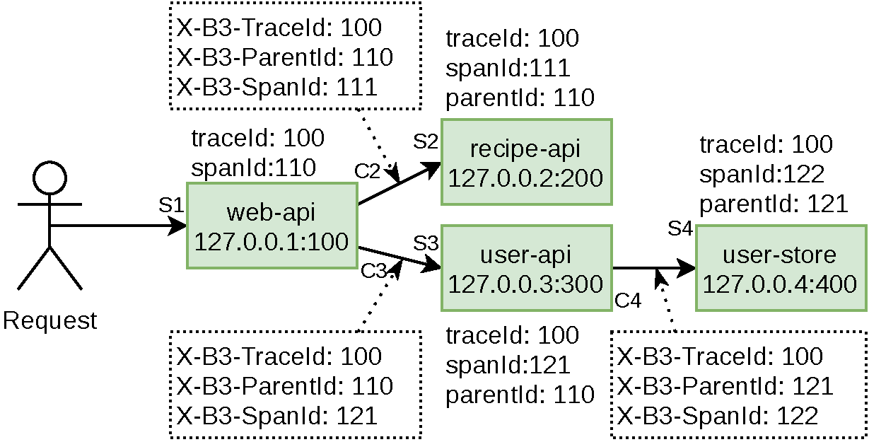
Figure 4-7. Example requests and Zipkin data
One concept that has been repeated a few times so far in this book is that a client will perceive one latency of a request, while a server will perceive another latency. A client will always determine that a request takes longer than the server. This is due to the time it takes a message to be sent over the network, plus other things that are hard to measure, such as a web server module automatically parsing a JSON request before user code can start measuring time.
Zipkin allows you to measure the difference in opinion between client and server. This is why the four requests in the example situation, marked as solid arrows in Figure 4-7, result in seven different message being sent to Zipkin. The first message, terminating with S1, only contains a server message. In this case, the third-party client isn’t reporting its perceived time, so there’s just the server message. For the three requests terminating in S2, S3, and S4, there is a correlating client message, namely C2, C3, and C4.
The different client and server messages can be sent from the different instances, asynchronously, and be received in any order. The Zipkin service will then stitch them each together and visualize the request hierarchy using the Zipkin web UI. The C2 message will looks something like this:
[{"id":"0000000000000111","traceId":"0000000000000100","parentId":"0000000000000110","timestamp":1579221096510000,"name":"get_recipe","duration":80000,"kind":"CLIENT","localEndpoint":{"serviceName":"web-api","ipv4":"127.0.0.1","port":100},"remoteEndpoint":{"ipv4":"127.0.0.2","port":200},"tags":{"http.method":"GET","http.path":"/recipe/42","diagram":"C2"}}]
These messages can be queued up by an application and occasionally flushed in batches to the Zipkin service, which is why the root JSON entry is an array. In Example 4-10, only a single message is being transmitted.
The client message and server message pairs will end up containing the same id, traceId, and parentId identifiers. The timestamp field represents the time when the client or server first perceived the request to start, and the duration is how long the service thought the request lasted. Both of these fields are measured in microseconds. The Node.js wall clock, attainable via Date.now(), only has millisecond accuracy, so it’s common to multiply that value by 1,000.1 The kind field is set to either CLIENT or SERVER, depending on which side of the request is being logged. The name field represents a name for the endpoint and should have a finite set of values (in other words, don’t use an identifier).
The localEndpoint field represents the service sending the message (so, the server with a SERVER message or the client with a CLIENT message). The service provides its own name in here, the port its listening on, and its own IP address. The remoteEndpoint field contains information about the other service (a SERVER message probably won’t know the client’s port, and likely won’t even know the client’s name).
The tags field contains metadata about the request. In this example, information about the HTTP request is provided as http.method and http.path. With other protocols, different metadata would be attached, such as a gRPC service and method name.
The identifiers sent in the seven different messages have been recreated in Table 4-2.
| Message | id |
parentId |
traceId |
kind |
|---|---|---|---|---|
S1 |
110 |
N/A |
100 |
SERVER |
C2 |
111 |
110 |
100 |
CLIENT |
S2 |
111 |
110 |
100 |
SERVER |
C3 |
121 |
110 |
100 |
CLIENT |
S3 |
121 |
110 |
100 |
SERVER |
C4 |
122 |
121 |
100 |
CLIENT |
S4 |
122 |
121 |
100 |
SERVER |
Apart from the messages sent to the server, the other important part of Zipkin is the metadata that is sent from client to server. Different protocols have different standards for sending this metadata. With HTTP, the metadata is sent via headers. These headers are provided by C2, C3, and C4 and are received by S2, S3, and S4. Each of these headers has a different meaning:
X-B3-TraceId-
Zipkin refers to all related requests as a Trace. This value is Zipkin’s concept of a Request ID. This value is passed between all related requests, unchanged.
X-B3-SpanId-
A Span represents a single request, as seen from both a client and a server (like C3/S3). Both the client and server will send a message using the same span ID.
X-B3-ParentSpanId-
A Parent Span is used for associating a child span with a parent span. This value is missing for the originating external request, but is present for deeper requests.
X-B3-Sampled-
This is a mechanism used for determining if a particular trace should be reported to Zipkin. For example, an organization may choose to track only 1% of requests.
X-B3-Flags-
This can be used to tell downstream services that this is a debug request. Services are encouraged to then increase their logging verbosity.
Essentially, each service creates a new span ID for each outgoing request. The current span ID is then provided as the parent ID in the outbound request. This is how the hierarchy of relationships is formed.
Now that you understand the intricacies of Zipkin, it’s time to run a local copy of the Zipkin service and modify the applications to interact with it.
Running Zipkin via Docker
Again, Docker provides a convenient platform for running the service. Unlike the other tools covered in this chapter, Zipkin provides an API and a UI using the same port. Zipkin uses a default port of 9411 for this.
Run this command to download and start the Zipkin service. It’s configured to keep trace information entirely in memory:
$docker run -p 9411:9411-it --name distnode-zipkinopenzipkin/zipkin-slim:2.19
Note that Zipkin should never be run in production in this manner, since the data is not persisted. For production use you would be better off running it directly on a machine.
Transmitting Traces from Node.js
For this example, you’re going to again start by modifying an existing application. Copy the web-api/consumer-http-basic.js file created in Example 1-6 to web-api/consumer-http-zipkin.js as a starting point. Modify the file to look like the code in Example 4-10.
Example 4-10. web-api/consumer-http-zipkin.js
#!/usr/bin/env node// npm install fastify@2 node-fetch@2 [email protected]constserver=require('fastify')();constfetch=require('node-fetch');constHOST=process.env.HOST||'127.0.0.1';constPORT=process.env.PORT||3000;constTARGET=process.env.TARGET||'localhost:4000';constZIPKIN=process.env.ZIPKIN||'localhost:9411';constZipkin=require('zipkin-lite');constzipkin=newZipkin({zipkinHost:ZIPKIN,serviceName:'web-api',servicePort:PORT,serviceIp:HOST,init:'short'});server.addHook('onRequest',zipkin.onRequest());server.addHook('onResponse',zipkin.onResponse());server.get('/',async(req)=>{req.zipkin.setName('get_root');consturl=`http://${TARGET}/recipes/42`;constzreq=req.zipkin.prepare();constrecipe=awaitfetch(url,{headers:zreq.headers});zreq.complete('GET',url);constproducer_data=awaitrecipe.json();return{pid:process.pid,producer_data,trace:req.zipkin.trace};});server.listen(PORT,HOST,()=>{console.log(`Consumer running at http://${HOST}:${PORT}/`);});
The zipkin-lite module is required and instantiated.
web-api accepts outside requests and can generate Trace IDs.
Hooks are called when requests start and finish.
Each endpoint will need to specify its name.
Outbound requests are manually instrumented.
Note
These examples use the zipkin-lite module. This module requires manual instrumentation, which is a fancy way of saying that you, the developer, must call different hooks to interact with the module. I chose it for this project to help demonstrate the different parts of the Zipkin reporting process. For a production app, the official Zipkin module zipkin would make for a better choice.
The consumer service represents the first service that an external client will communicate with. Because of this, the init configuration flag has been enabled. This will allow the service to generate a new Trace ID. In theory, a reverse proxy can be configured to also generate initial identifier values. The serviceName, servicePort, and serviceIp fields are each used for reporting information about the running service to Zipkin.
The onRequest and onResponse hooks allow the zipkin-lite module to interpose on requests. The onRequest handler runs first. It records the time the request starts, and injects a req.zipkin property that can be used throughout the life cycle of the request. Later, the onResponse handler is called. This then calculates the overall time the request took, and sends a SERVER message to the Zipkin server.
Within a request handler, two things need to happen. The first is that the name of the endpoint has to be set. This is done by calling req.zipkin.setName(). The second is that for each outbound request that is sent, the appropriate headers need to be applied and that the time the request took should be calculated. This is done by first calling req.zipkin.prepare(). When this is called, another time value is recorded, and a new span ID is generated. This ID, and the other necessary headers, are provided in the returned value, which is assigned here to the variable zreq.
These headers are then provided to the request via zreq.headers. Once the request is complete, a call to zreq.complete() is made, passing in the request method and URL. Once this happens, the overall time taken in calculated, and the CLIENT message is then sent to the Zipkin server.
Next up, the producing service should also be modified. This is important because not only should the timing perceived by the client be reported (web-api in this case), but also the timing from the server’s point of view (recipe-api). Copy the recipe-api/producer-http-basic.js file created in Example 1-5 to recipe-api/producer-http-zipkin.js as a starting point. Modify the file to look like the code in Example 4-11. Most of the file can be left as is, so only the required changes are displayed.
Example 4-11. recipe-api/producer-http-zipkin.js (truncated)
constPORT=process.env.PORT||4000;constZIPKIN=process.env.ZIPKIN||'localhost:9411';constZipkin=require('zipkin-lite');constzipkin=newZipkin({zipkinHost:ZIPKIN,serviceName:'recipe-api',servicePort:PORT,serviceIp:HOST,});server.addHook('onRequest',zipkin.onRequest());server.addHook('onResponse',zipkin.onResponse());server.get('/recipes/:id',async(req,reply)=>{req.zipkin.setName('get_recipe');constid=Number(req.params.id);
Example 4-11 doesn’t act as a root service, so the init configuration flag has been omitted. If it receives a request directly, it won’t generate a trace ID, unlike the web-api service. Also, note that the same req.zipkin.prepare() method is available in this new recipe-api service, even though the example isn’t using it. When implementing Zipkin within services you own, you’ll want to pass the Zipkin headers to as many upstream services as you can.
Be sure to make both of the files executable, and run the npm install [email protected] command in both directories.
Once you’ve created the two new service files, run them and then generate a request to the web-api by running the following commands:
$node recipe-api/producer-http-zipkin.js$node web-api/consumer-http-zipkin.js$curl http://localhost:3000/
A new field, named trace, should now be present in the output of the curl command. This is the trace ID for the series of requests that have been passed between the services. The value should be sixteen hexadecimal characters, and in my case, I received the value e232bb26a7941aab.
Visualizing a Request Tree
Data about the requests have been sent to your Zipkin server instance. It’s now time to open the web interface and see how that data is visualized. Open the following URL in your browser:
http://localhost:9411/zipkin/
You should now be greeted with the Zipkin web interface. It’s not too exciting just yet. The left sidebar contains two links. The first one, which looks like a magnifying glass, is to the current Discover screen. The second link, resembling network nodes, links to the Dependencies screen. At the top of the screen is a plus sign, which can be used for specifying which requests to search for. With this tool you can specify criteria like the service name or tags. But, for now you can ignore those. In the upper right corner is a simple search button, one that will display recent requests. Click the magnifying glass icon, which will perform the search.
Figure 4-8 is an example of what the interface should look like after you’ve performed a search. Assuming you ran the curl command just once, you should only see a single entry.
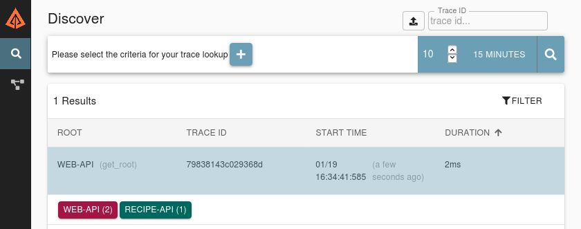
Figure 4-8. Zipkin discover interface
Click the entry to be taken to the timeline view page. This page displays content in two columns. The column on the left displays a timeline of requests. The horizontal axis represents time. The units on the top of the timeline display how much time has passed since the very first SERVER trace was made with the given trace ID. The vertical rows represent the depth of the request; as each subsequent service makes another request, a new row will be added.
For your timeline, you should see two rows. The first row was generated by the web-api, and has a call named get_root. The second row was generated by the recipe-api, and has a call named get_recipe. A more complex version of the timeline you’re seeing, based on the previously mentioned more complex system with an additional user-api and user-store, is displayed in Figure 4-9.
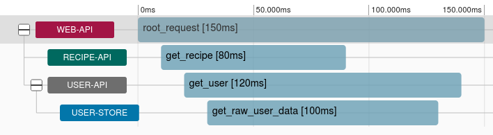
Figure 4-9. Example Zipkin trace timeline
Click the second row. The right column will be updated to display additional metadata about the request. The Annotations bar displays a timeline for the span you clicked. Depending on the speed of the request, you will see between two and four dots. The furthest left and furthest right dots represents the time that the client perceived the request to take. If the request was slow enough you should see two inner dots, and those will represent the time the server perceived the request to take. Since these services are so fast, the dots might overlap and will be hidden by the Zipkin interface.
The Tags section displays the tags associated with the request. This can be used to debug which endpoints are taking the longest time to process, and which service instances (by using the IP address and port) are to blame.
Visualizing Microservice Dependencies
The Zipkin interface can also be used to show aggregate information about the requests that it receives. Click the Dependencies link in the sidebar to be taken to the dependencies screen. The screen should be mostly blank, with a selector at the top to specify a time range and perform a search. The default values should be fine, so click the magnifying glass icon to perform a search.
The screen will then be updated to display two nodes. Zipkin has searched through the different spans it found that matched the time range. Using this information it has determined how the services are related to each other. With the two example applications, the interface isn’t all that interesting. You should see a node on the left representing the web-api (where requests originate), and on the right a node representing the recipe-api (the deepest service in the stack). Small dots move from the left of the screen to the right, showing the relative amount of traffic between the two nodes.
If you were using Zipkin with many different services within an organization, you would see a much more complex map of the relationships between services. Figure 4-10 is an example of what the relationships between the four services in the more complex example would look like.
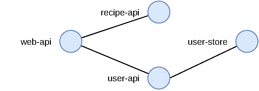
Figure 4-10. Example Zipkin dependency view
Assuming every service within an organization uses Zipkin, such a diagram would be a very powerful tool for understanding the interconnections between services.
Health Checks
“Load Balancing and Health Checks” looked at how HAProxy can be configured to automatically remove and re-add a running service instance to the pool of candidate instances for routing requests to. HAProxy can do this by making an HTTP request to an endpoint of your choosing and checking the status code. Such an endpoint is also useful for checking the liveness of a service—which is a term meaning a newly-deployed service has finished the startup stage and is ready to receive requests (like establishing a database connection). Kubernetes, which is covered in [Link to Come], can also make use of such a liveness check. It is generally useful for an application to know if it’s healthy or not.
An application can usually be considered healthy if it is able to respond to incoming requests with correct data, and without ill side effects. The specifics of how to measure this will change depending on the application. If an application needs to make a connection to a database, and such a connection is lost, then the application probably won’t be able to process the requests it receives (note that your application should attempt to reconnect to databases, this is covered in [Link to Come]). In such a case it would make sense to have the application declare itself unhealthy.
On the other hand, some features are a bit of a grey area. For example, if a service is unable to establish a connection to a caching service, but is still able to connect to a database and serve requests, it is probably fine to declare itself as healthy. The grey area in this case is with response time. If the service is no longer able to achieve its SLA, then it might be dangerous to run as it could cost your organization money. In this situation it might make sense to declare the service as being degraded.
What would happen in this situation if the degraded service were to declare itself unhealthy? The service might be restarted by some sort of deployment management tool. But, if the problem is that the caching service is down, then perhaps every single service would be restarted. This can lead to situations where no service is available to serve requests. This scenario will be covered in “Alerting with Cabot”. For now, consider slow/degraded services healthy.
Health checks are usually run periodically. Sometimes they are triggered by a request from an external service, such as HAProxy making an HTTP request (an operation that defaults to every two seconds). Sometimes they are triggered internally, such as a setInterval() call that checks the application’s health before reporting to an external discovery service like Consul that it is healthy (a check that runs perhaps every ten seconds). In any case, the overhead of running the health check should not be so high that the process is slowed down or the database is overwhelmed.
Building a Health Check
In this section you will build a health check for a rather boring service. This application will have both a connection to a Postgres database, resembling a persistent data store, as well as a connection to Redis, which will represent a cache.
Before you start writing code, you’ll need to run the two backing services. Run the commands in Example 4-12 to get a copy of Postgres and Redis running. You’ll need to run each command in a new terminal window. Ctrl+C can be used to kill either service.
Example 4-12.
$docker run--rm-p 5432:5432-ePOSTGRES_PASSWORD=hunter2-ePOSTGRES_USER=tmp-ePOSTGRES_DB=tmppostgres:12.3$docker run--rm-p 6379:6379redis:6.0
Next, create a new file from scratch named basic-http-healthcheck.js. Insert the content from Example 4-13 into your newly created file.
Example 4-13. basic-http-healthcheck.js
#!/usr/bin/env node// npm install fastify@2 ioredis@4 pg@7constserver=require('fastify')();constHOST='0.0.0.0';constPORT=3300;constredis=new(require("ioredis"))({enableOfflineQueue:false});letpg=new(require('pg').Client)();pg.connect();// Note: Postgres will not reconnect on failureserver.get('/health',async(req,reply)=>{try{constres=awaitpg.query('SELECT $1::text as status',['ACK']);if(res.rows[0].status!=='ACK')reply.code(500).send('DOWN');}catch(e){reply.code(500).send('DOWN');}// ... other down checks ...letstatus='OK';try{if(awaitredis.ping()!=='PONG')status='DEGRADED';}catch(e){status='DEGRADED';}// ... other degraded checks ...reply.code(200).send(status);});server.listen(PORT,HOST,console.log(`http://${HOST}:${PORT}/`));
Redis requests will fail when offline.
Completely fail if Postgres cannot be reached.
Pass with a degraded state if Redis cannot be reached.
This file makes use of the ioredis module for connecting to and issuing queries for Redis. It also makes use of the pg module for working with Postgres. When ioredis is instantiated it will default to connecting to a locally running service, which is why connection details aren’t necessary. The enableOfflineQueue flag specifies if commands should be queued up when the Node.js process can’t connect to the Redis instance. It defaults to true, meaning requests can be queued up. Since Redis is being used as a caching service, and not as a primary data store, the flag should set to false, otherwise a queued up request to access the cache could be slower than connecting to the real data store.
The pg module also defaults to connecting to a Postgres instance running locally, but it will still need some connection information. That will be provided using environment variables.
This health check endpoint is configured to first check for features that are critical to run. If any of those features are lacking then the endpoint will immediately fail. In this case, only the Postgres check applies, but a real application might have more. After that are the checks that will result in a degraded service are run. Only the Redis check applies in this situation. Both of these checks work by querying the backing store and checking for a sane response.
Note that a degraded service will return a 200 status code. HAProxy could, for example, be configured to still direct requests to this service. If the service is degraded, then an alert could be generated (see “Alerting with Cabot”). Figuring our why the cache isn’t working is something that our application shouldn’t be concerned about. The issue might be that Redis itself has crashed or that there is a network issue.
Now that the service file is ready, run the following command to start the service:
$ PGUSER=tmpPGPASSWORD=hunter2PGDATABASE=tmpnode basic-http-healthcheck.js
The Postgres connection variables have been provided as environment variables and are used by the underlying pg module. Explicitly naming the variables in code is a better approach for production code, and these variables are only used for brevity.
Now that your service is running, it’s time to try using the health checks.
Testing the Health Check
With the process running and connecting to the databases it should be considered in a healthy state. Issue the following request to check the status of the application:
$ curl -v http://localhost:3300/health
The response should contain the message OK, and have an associated 200 status code.
Now we can simulate a degraded situation. Switch focus to the Redis service and press Ctrl+C to kill the process. You should see some error messages printed from the Node.js process. They will start off quickly then slow down as the ioredis module uses exponential backoff when attempting to reconnect to the Redis server. This means that it retries rapidly and then slows down.
Now that the application is no longer connected to Redis, run the same curl command again. This time, the response body should contain the message DEGRADED, though it will still have a 200 status code.
Switch back to the terminal window you previously ran Redis with. Start the Redis service again, then switch back to the terminal where you ran curl, and run the request again. Depending on your timing, you might still receive the DEGRADED message, but you will eventually get the OK message once ioredis is able to reestablish a connection.
Note that killing Postgres in this manner will cause the application to crash. The pg library doesn’t provide the same automatic reconnection feature that ioredis provides. Additional reconnection logic will need to be added to the application to get that working. [Link to Come] contains an example of this.
Alerting with Cabot
There are certain issues that simply cannot be resolved by automatically killing and restarting a process. Issues related to stateful services, like the downed Redis service mentioned in the previous section, is one such example. Elevated 5XX error rates is another common example. In these situations its often necessary to alert a developer to find the root cause of an issue and correct it. If such errors can cause a loss of revenue then it becomes necessary to wake developers up in the middle of the night.
In these situations a cellphone is usually the best medium for waking a developer, often by triggering an actual phone call. Other message formats, such as emails, chat room messages, and text messages, usually aren’t accompanied by an annoying ringing sound, and often won’t suffice for alerting the developer.
In this section you’ll set up an instance of Cabot, which is an open source tool for polling the health of an application and triggering alerts. Cabot supports multiple forms of health checks, such as querying Graphite and comparing reported values to a threshold, as well as pinging a host. Cabot also supports making an HTTP request, which is what is covered in this section.
In this section you’ll also create a free Twilio trial account. Cabot can use this account to both send SMS messages and make phone calls. You can skip this part if you would prefer not to create a Twilio account. In that case you’ll just see a dashboard changing colors from a happy green to an angry red.
The examples in this section will have you create a single user in Cabot, and that user will receive all the alerts. In practice an organization will setup schedules, usually referred to as the on-call rotation. In these situations the person who will receive an alert will depend on the schedule. For example, Alice might be on call week one, Bob on week two, Carol on week three, and back to Alice for week four.
Note
Another important feature in a real organization is something called a Runbook. A runbook is usually a page in a wiki and is associated with a given alert. The runbook contains information on how to diagnose and fix an issue. That way, when an engineer gets an alert at 2 A.M. about the Database Latency alert, they can read about how to access the database and run a query. You won’t create a runbook for this example, but you must be diligent in doing so for real-world alerts.
Create a Twilio Trial Account
At this point, head over to twilio.com, and create a trial account. When you create an account, you will get two pieces of data that you will need for configuring Cabot. The first piece of information is called an Account SID. This is a string that starts with AC and contains a bunch of hexadecimal characters. The second piece of information is the Auth Token. This value just looks like normal hexadecimal characters.
Using the interface, you’ll also need to configure a Trial Number. This is a virtual phone number that you can use with this project. The phone number begins with a plus sign, then a country code, then the rest of the number. You’ll need to use this number within your project, including the plus sign and country code. The number you receive might look like +15558675309.
And finally, you’ll need to configure your personal cellphone’s phone number to be a Verified Number / Verified Caller ID in Twilio. This allows you to confirm with Twilio that the phone number you have belongs to you and that you’re not just using Twilio to send spam texts to strangers, a process which is a limitation of the Twilio trial account. Once you verify your phone number you’ll later be able to configure Cabot to send an SMS message to it.
Running Cabot via Docker
Cabot is a little more complex than the other services covered in this chapter. It requires several Docker images, not just a single one. For that reason you’ll need to use Docker Compose to launch several containers, instead of launching a single one using Docker. Run the following commands to pull the git repository and checkout a commit that is known to be compatible with this example:
$git clone [email protected]:cabotapp/docker-cabot.git cabot$cdcabot$git checkout cdb72e
Next, create a new file located at conf/production.env within this repository (note that it’s not within the distributed-node directory that you’ve been creating all your other project files in). Add the content from Example 4-14 to this file.
Example 4-14. config/production.env
TIME_ZONE=America/Los_AngelesADMIN_EMAIL=[email protected]CABOT_FROM_EMAIL=[email protected]DJANGO_SECRET_KEY=abcd1234WWW_HTTP_HOST=localhost:5000WWW_SCHEME=http# GRAPHITE_API=http://<YOUR-IP-ADDRESS>:8080/TWILIO_ACCOUNT_SID=<YOUR_TWILIO_ACCOUNT_SID>TWILIO_AUTH_TOKEN=<YOUR_TWILIO_AUTH_TOKEN>TWILIO_OUTGOING_NUMBER=<YOUR_TWILIO_NUMBER>
Set this value to your TZ Time Zone.
For extra credit, configure a Graphite source using your IP Address.
Omit these lines if you’re not using Twilio. Be sure to prefix the phone number with a plus sign and country code.
Tip
If you’re feeling adventurous, configure the GRAPHITE_API line to use the same Graphite instance that you created in “Metrics with Graphite, StatsD, and Grafana”. Later, when using the Cabot interface, you can then choose which metrics to create an alert on. This is useful for taking a metric, like request timing, and alerting once it surpasses a certain threshold, such as 200ms. However, for brevity, this section won’t cover how to set it up, and you can omit the line.
Once you’ve finished configuring Cabot, run the following command to start the Cabot service:
$ docker-compose upThis will cause several Docker containers to start running. In the terminal you should see progress as each image is downloaded, followed by colored output associated with each container once they’re running. Once things have settled down you’re ready to move on to the next step.
Creating a Health Check
For this example, use the same basic-http-healthcheck.js file from Example 4-13 that you made in the previous section. Execute that file, and also run the Postgres service as configured in Example 4-12. Once that is done Cabot can be configured to make use of the /health endpoint the Node.js service exposes.
With the Node.js service now running, open the Cabot web service using your web browser by visiting localhost:5000.
You’ll first be prompted to create an administrative account. Use the default username of admin. Next, put in your email address and a password, then click Create. Then, you’ll be prompted to login. Type admin for the username field, enter your password again, then click Log in. You’ll finally be taken to the services screen that will contain no entries.
On the empty services screen, click the large plus symbol to be taken to the New service screen. Then, input the information from Table 4-3 into the create service form.
Name |
Dist Node Service |
Url |
http://<LOCAL_IP>:3300/ |
Users to notify |
admin |
Alerts |
Twilio SMS |
Alerts enabled |
checked |
Again, you’ll need to substitute <LOCAL_IP> with your IP address. Once you’ve entered the information, click the Submit button. This will take you to a screen where you can view the Dist Node Service overview.
On this screen, scroll down to the Http checks section, and click the plus sign to be taken to the ----tpcheck/create/?instance=&service=1[New check screen. On this screen, input the information from Table 4-4 into the create check form.
Name |
Dist Node HTTP Health |
Endpoint |
http://<LOCAL_IP>:3300/health |
Status code |
200 |
Importance |
Critical |
Active |
checked |
Service set |
Dist Node Service |
Once you’ve entered that information, click the Submit button. This will take you back to the Dist Node Service overview screen.
Next, the admin account needs to be configured to receive alerts using Twilio SMS. In the upper right corner of the screen, click the admin drop down, then click Profile settings. On the left sidebar, click the Twilio Plugin link. This form will ask you for your phone number. Enter your phone number, beginning with a plus symbol and the country code. This number should match the verified number that you previously entered in your Twilio account. Once you’re done click the Submit button.
Once you’re done setting your phone number, click the Checks link in the top navigation bar. This will take you to the Checks listing page, which should contain the one entry you’ve created. Click the single entry, Dist Node HTTP Health, to be taken to the health check history listing. At this point you should only see one or two entries as they run once every five minutes. These entries should have a green succeeded label next to them. Click the circular arrow icon in the upper right to trigger another health check.
Now, switch back to the terminal window where your Node.js service is running. Kill it with Ctrl+C. Then, switch back to Cabot and click the icon to run the test again. This time the test will fail, and you’ll get a new entry in the list with a red background and the word failed.
You should also get a text message containing information about the alert. The message I received is shown here:
Sent from your Twilio trial account - Service
Dist Node Service reporting CRITICAL status:
http://localhost:5000/service/1/
If Cabot were properly installed on a real server somewhere with a real hostname, the text message would contain a working link that could then be opened on your phone. However, since Cabot is probably running on your laptop, the URL doesn’t make a lot of sense in this context.
Click the Services link at the top of the screen, then click the Dist Node Service link again. On this screen you’ll now see a graph displaying the status of the service, as well as a banner stating that the service is critical, like in Figure 4-11. Now click the Acknowledge alert button to pause the alerts for 20 minutes. This is useful for giving you time to work on the issue without being alerted over and over. It’s now time to fix the failing service.
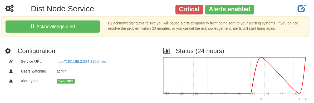
Figure 4-11. Cabot service status screenshot
Switch back to the terminal where you ran the Node.js process and start it again. Then, switch back to the browser. Navigate back to the Http check you created. Click the icon to trigger the check again. This time the check should succeed, and it will switch back to a green succeeded message.
Cabot, as well as other alerting tools, offers the ability to assign different users to different services. This is important since within an organization different teams will own different services. When you created an HTTP alert, it was also possible to provide a regex to be applied against the body. This can be used to differentiate a degraded service from an unhealthy service. Cabot can then be configured to have an unhealthy service alert an engineer, but have a degraded services merely be highlighted in the UI.
1 Note that process.hrtime() is only useful for getting relative time, and can’t be used to get the current time with microsecond accuracy.