
Chapter 7
Challenges Ahead Risk-Based AC Optimal Power Flow Under Uncertainty for Smart Sustainable Power Systems
Florin Capitanescu
Researcher, Luxembourg Institute of Science and Technology (LIST), Environmental Research and Innovation (ERIN) Department, Belvaux, Luxembourg
7.1 Chapter Overview
In order to meet the ambitious long-term sustainability objectives set by governments, most electric power systems worldwide are undergoing significant structural and operational changes due to mainly the large-scale integration of intermittent renewable generation (wind, solar, etc.) and the increasing adoption of emerging flexibility-enabling technologies (storage batteries, HVDC links, etc.). This challenging energy transition toward smarter sustainable power systems requires in turn adapting decision making tools (e.g., for planning, operational planning, and real-time control) to cope with the prevailing operational environment.
This chapter focuses on optimal power flow (OPF) which, together with unit commitment and dynamic simulation-based stability control, are the main decision making problems to be solved in day-ahead operational planning. The chapter discusses the challenges and proposes solutions to leverage OPF computations for future smart sustainable power systems, fostering the development of the first generation of tools balancing risk-based security criteria and renewable generation forecast uncertainty. It describes the stages needed to reach this goal and details the contents of their corresponding building blocks. Illustrative examples using a small test system are used through the whole chapter to support the various concepts presented.
The chapter is organized as follows. Section 7.2 revisits the conventional (deterministic) OPF problem. Section 7.3 presents a formulation of the OPF problem that integrates a probabilistic, risk-based security criterion. Section 7.4 addresses the extension of the OPF framework to take into account renewable generation forecast uncertainty. Finally, Section 7.5 is devoted to advanced issues related to the current and future generation of OPF packages.
7.2 Conventional (Deterministic) AC Optimal Power Flow (OPF)
7.2.1 Introduction
Initiated in the early 1960s [1], AC optimal power flow (OPF) calculations are nowadays fundamental in power systems planning, operational planning, operation, control, and electricity markets [2–7].
OPF problems search for optimal values for a set of decision variables, according to a certain objective, while ensuring power system static security (i.e., satisfying grid power flow equations and other operational constraints with respect to both the base case and a set of plausible contingencies). The consideration of contingency constraints (e.g., the N-1 security criterion, an operating rule to be enforced by transmission system operators) is vital for practical applications and represents by far the most important and challenging requirement for industrial OPF software [2–6]. However, although this OPF challenge has been expressed for over fifty years [8], most research endeavors ignore it. This presentation asserts that contingency constraints make it intrinsically part of the OPF problem, a concept that has also been named in the literature as security-constrained optimal power flow (SCOPF) or, as a notable special case, security-constrained economic dispatch (SCED).
OPF requirements, challenges, and solution methodologies have been the subject of an important number of survey papers stemming from teams of experts with different backgrounds (industry, academia, and software developers) [2–6], out of which the recent paper [2] is absolutely outstanding while [6] provides a critical review of latest developments in this area.
7.2.2 Abstract Mathematical Formulation of the OPF Problem
OPF is in its general form a non-convex, nonlinear, large-scale, static optimization problem with both continuous and discrete variables. Because OPF is very versatile in terms of optimization goals (e.g., secure economic dispatch, minimum cost/number of control means re-dispatch, minimum power losses, maximum reactive power reserves, etc.) and the means to fulfill them, it requires careful problem formulation. An abstract traditional OPF problem formulation is as follows [2, 3, 5]:
where subscripts 0 and ![]() denote the base case (or pre-contingency state) and post-contingency state, respectively;
denote the base case (or pre-contingency state) and post-contingency state, respectively; ![]() is the number of postulated contingencies;
is the number of postulated contingencies; ![]() ,
, ![]() are the sets of state variables (i.e., real and imaginary parts of bus voltages) in the pre-contingency state and post-contingency state (i.e., after the corrective actions took place), respectively;
are the sets of state variables (i.e., real and imaginary parts of bus voltages) in the pre-contingency state and post-contingency state (i.e., after the corrective actions took place), respectively; ![]() is the set of preventive controls (e.g., generator active powers, generator voltages, taps position of phase shifter and on load tap changing transformer, etc.);
is the set of preventive controls (e.g., generator active powers, generator voltages, taps position of phase shifter and on load tap changing transformer, etc.); ![]() is the set of corrective controls (e.g., generator active powers, generator voltages, etc.);
is the set of corrective controls (e.g., generator active powers, generator voltages, etc.); ![]() is the objective function to be minimized (e.g., cost of generation dispatch, power losses, etc.); functions
is the objective function to be minimized (e.g., cost of generation dispatch, power losses, etc.); functions ![]() model mainly the AC power flow network equations in state
model mainly the AC power flow network equations in state ![]() ; functions
; functions ![]() model the operational limits (e.g., mainly on branch currents and voltage magnitudes) in state
model the operational limits (e.g., mainly on branch currents and voltage magnitudes) in state ![]() ; and
; and ![]() is the set of allowed variations of corrective actions (according to their ramping ability and alloted time for control).
is the set of allowed variations of corrective actions (according to their ramping ability and alloted time for control).
The objective (7.1) considers the cost of base case operation. The constraints (7.2), (7.3) and (7.4), (7.5) enforce the feasibility of the base-case and post-contingency states, respectively. The constraints (7.6) impose ranges on corrective actions.
OPF can be used to cover the static power system security according to any of the following modes:
- preventive security [8]: only preventive actions are taken to ensure that in the event of a contingency, no operational limit (e.g., branch currents and voltage magnitudes) will be violated;
- also corrective security [9]: both preventive and corrective actions ensure that, if a contingency occurs, violated limits can be removed without loss of load.
7.2.3 OPF Solution via Interior-Point Method
For the sake of simplicity1 it is assumed that (i) the OPF formulation (7.1)–(7.6) contains only continuous variables, leading to a nonlinear programming (NLP) problem, and (ii) the size of the problem allows the direct solution via an NLP method.
Several notable approaches proposed in the literature for solving NLP OPF problems are today the core of various commercial OPF software (e.g., chronologically [3]: sequential linear programming (SLP) [10], sequential quadratic programming (SQP) [11], Newton method [12], interior-point method (IPM) [13, 14], etc.)
Since the early 1990s, the IPM has gained increasingly significant popularity in the power systems community owing to three major advantages: (i) ease of handling inequality constraints by logarithmic barrier functions, (ii) speed of convergence, and (iii) a feasible initial point is not required [13–17].
The basics of IPM are briefly detailed in what follows.
7.2.3.1 Obtaining the Optimality Conditions In IPM
The abstract OPF formulation (7.1)–(7.6) can be compactly written as follows:
where ![]() ,
, ![]() , and
, and ![]() are twice continuously differentiable functions,
are twice continuously differentiable functions, ![]() is a vector grouping both decision variables and state variables, the vectors
is a vector grouping both decision variables and state variables, the vectors ![]() ,
, ![]() , and
, and ![]() having sizes
having sizes ![]() ,
, ![]() , and
, and ![]() , respectively.
, respectively.
The IPM requires four steps to obtain optimality conditions as follows.
First step: slack variables are added to inequality constraints, transforming them into equality constraints and non-negativity conditions on slacks:
where the vectors ![]() and
and ![]() are called primal variables.
are called primal variables.
Second step: the non-negativity conditions are added to the objective function as logarithmic barrier terms, leading to an equality constrained optimization problem:
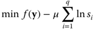
where ![]() is a positive scalar called the barrier parameter, whose key role in IPM will be explained later on.
is a positive scalar called the barrier parameter, whose key role in IPM will be explained later on.
Third step: the equality constrained optimization problem is transformed into an unconstrained one, by building the Lagrangian:
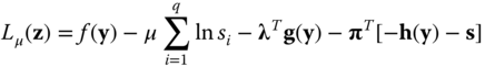
where the vectors of Lagrange multipliers ![]() and
and ![]() are called dual variables and the vector
are called dual variables and the vector ![]() gathers all variables, that is,
gathers all variables, that is, ![]() .
.
Fourth step: the perturbed Karush–Kuhn–Tucker (KKT) first order necessary optimality conditions of the problem are obtained by setting to zero the derivatives of the Lagrangian with respect to all variables [18]:
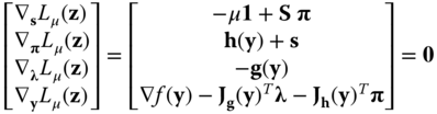
where ![]() is a diagonal matrix of slack variables,
is a diagonal matrix of slack variables, ![]() is the gradient of
is the gradient of ![]() ,
, ![]() is the Jacobian of
is the Jacobian of ![]() , and
, and ![]() is the Jacobian of
is the Jacobian of ![]() .
.
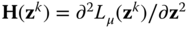
Central to the IPM is the theorem [18], which proves that as ![]() tends to zero the solution
tends to zero the solution ![]() converges to a local optimum of the original problem (7.7), (7.8). IPM solution algorithms (e.g., pure primal dual [13–15], predictor-corrector [13–15], multiple centrality corrections [16, 17]) exploit this finding, solving the perturbed KKT optimality conditions (7.13) while gradually decreasing
converges to a local optimum of the original problem (7.7), (7.8). IPM solution algorithms (e.g., pure primal dual [13–15], predictor-corrector [13–15], multiple centrality corrections [16, 17]) exploit this finding, solving the perturbed KKT optimality conditions (7.13) while gradually decreasing ![]() to zero as iterations progress. To facilitate understanding, the basic primal dual IPM algorithm is outlined hereafter.
to zero as iterations progress. To facilitate understanding, the basic primal dual IPM algorithm is outlined hereafter.
7.2.3.2 The Basic Primal Dual Algorithm
- 1. Set iteration count
 . Chose
  . Initialize
  such that slack variables and their corresponding dual variables are strictly positive
 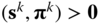 .
. - 2. Solve the linearized KKT conditions (7.13) for the Newton direction
 :
7.14
:
7.14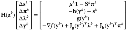
- where
 is the second derivatives Hessian matrix.
 - 3.
Compute the maximum step length
 along the Newton direction
  such that
  :7.15
:7.15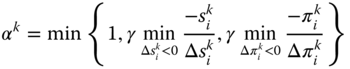
where
 is a safety factor2
 - aiming to maintain the strict positiveness of slack variables and their corresponding dual variables.
-
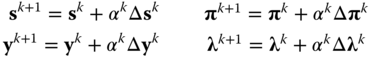
Update the solution:
- 4. Convergence test. A locally optimal solution is found and the optimization process terminates when change in primal feasibility, scaled dual feasibility, scaled complementarity gap and objective function from one iteration to the next meet some tolerances (typically
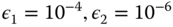 ) [13–15]:
7.16
) [13–15]:
7.16 7.17
7.17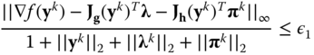 7.18
7.18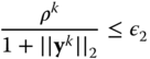 7.19
7.19
- where
 is the complementarity gap.
 - 5.
Update the barrier parameter:

where the centering parameter is usually set as
 .
.Set
 and go back to step 2.
As with any approach, the IPM has also some drawbacks: (i) the heuristic to decrease the barrier parameter, (ii) the positivity condition on slack variables and their dual variables, which may shorten the Newton step length, slowing down convergence, and (iii) lack of efficient warm/hot start, which should generally further speed-up OPF solution methodologies (see Figure 7.3).
7.2.4 Illustrative Example
7.2.4.1 Description of the Test System
The main characteristics of the abstract OPF formulation are best unveiled for educational purposes on a small system. Figure 7.1 sketches a 5-bus system, inspired from [19], whose bus and line data are provided in Tables 7.1 and 7.2, respectively.
Figure 7.1 One-line diagram of the 5-bus system.
In Table 7.1, all notations are self-explanatory, except of ![]() which denotes the ramping ability of a generator (both up and down) as a corrective control action for the assumed time horizon for removing post-contingency violated limits.
which denotes the ramping ability of a generator (both up and down) as a corrective control action for the assumed time horizon for removing post-contingency violated limits.
Table 7.1 5-bus system data and initial state
| Bus | MW | MVar | MW | MVar | pu | pu | pu | MW | MW | MVar | MVar | MW |
| 1 | 1100 | 400 | − | − | 0.954 | 0.92 | 1.05 | − | − | − | − | − |
| 2 | 500 | 200 | − | − | 0.950 | 0.92 | 1.05 | − | − | − | − | − |
| 3 | − | − | 700.0 | 69.5 | 1.0 | 0.92 | 1.05 | 150 | 1500 | −500 | 750 | 200 |
| 4 | − | − | 600.0 | 304.9 | 1.0 | 0.92 | 1.05 | 150 | 1500 | −500 | 750 | 200 |
| 5 | − | − | 333.8 | 146.9 | 1.0 | 0.92 | 1.05 | 150 | 1500 | −500 | 750 | 200 |
In Table 7.2, ![]() ,
, ![]() , and
, and ![]() are the resistance, the reactance, and the susceptance, respectively, of the line linking bus
are the resistance, the reactance, and the susceptance, respectively, of the line linking bus ![]() and bus
and bus ![]() . Note that the line current limit
. Note that the line current limit ![]() (in A) corresponds to 1100 MVA limit and hence to 11 pu current limit in 100 MVA base.
(in A) corresponds to 1100 MVA limit and hence to 11 pu current limit in 100 MVA base.
Table 7.2 5-bus system: line data
| Bus | Bus | ||||||
| Line | kV | A | |||||
| L1 | 1 | 2 | 400 | 3.2 | 16 | 160 | 1587.7 |
| L2 | 1 | 3 | 400 | 6.4 | 32 | 320 | 1587.7 |
| L3 | 1 | 4 | 400 | 3.2 | 16 | 160 | 1587.7 |
| L4 | 2 | 5 | 400 | 6.4 | 32 | 320 | 1587.7 |
| L5 | 3 | 4 | 400 | 6.4 | 32 | 320 | 1587.7 |
| L6 | 4 | 5 | 400 | 6.4 | 32 | 320 | 1587.7 |
The following generator cost curves, in (US) ![]() , are assumed:
, are assumed:
![]() ,
,
![]() ,
,
![]() .
.
For the sake of simplicity, current and voltage limits are considered the same in both pre-contingency and post-contingency states. Furthermore, only N-1 lines outages are considered in the contingencies set, hence ![]() . The contingencies are named according to the disconnected line (e.g., L1, L2, L3, L4, L5, and L6).
. The contingencies are named according to the disconnected line (e.g., L1, L2, L3, L4, L5, and L6).
7.2.4.2 Detailed Formulation of the OPF Problem
The compact OPF formulation (7.1)–(7.6) is specifically detailed hereafter for the 5-bus system, adopting a rectangular coordinates model for complex bus voltages:
where ![]() is the voltage magnitude at bus
is the voltage magnitude at bus ![]() .
.
The formulation models the most comprehensive operating mode, that is, “also corrective” (see Table 7.3); the simplifying assumptions behind the other modes are explained later on.
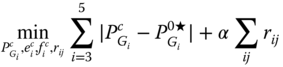
The objective (7.1) is economic dispatch (i.e., minimum generation cost):
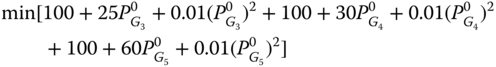
The decision variables of this problem are generator active powers and generator voltages, which are limited within some ranges (7.26) and (7.27), respectively.
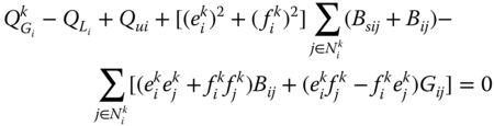
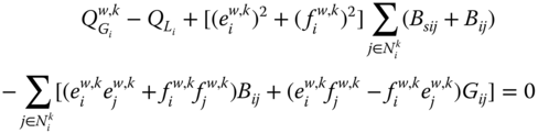
Equality constraints (7.2) and (7.4) comprise mainly the active and reactive power flow equations at each bus (![]() ) and for each system state (
) and for each system state (![]() ):
):
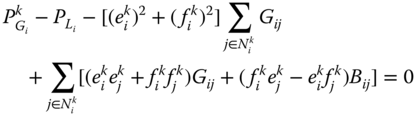
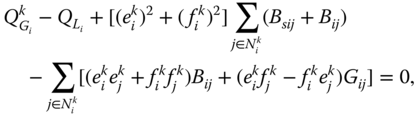
where ![]() is the set of adjacent buses to bus
is the set of adjacent buses to bus ![]() in state
in state ![]() , other notations being self-explanatory.
, other notations being self-explanatory.
The reference3 voltage angle is set at bus 5:
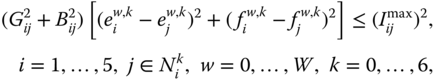
Inequality constraints (7.3) and (7.5) include operational limits on (longitudinal) branch current, voltage magnitude, and generator reactive power:
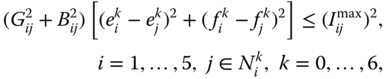
and limits on decision variables:
Finally, the coupling constraints (7.6) take on the form:

Note that, for the sake of formulation simplicity, the branch current is approximated by the longitudinal current in (7.23).
7.2.4.3 Analysis of Various Operating Modes
Table 7.3 provides, for various operating modes, the values of the objective, the six decision variables, and the critical (i.e., violated, binding, or near-binding) operation constraints in post-contingency states.
Table 7.3 Values of the objective, decision variables, and critical post-contingency constraints for various operating modes
| Objective | Decision variables | Critical constraints | |||||||||
| Operating | cost | ||||||||||
| modes | MW | MW | MW | pu | pu | pu | pu | pu | pu | pu | |
| unoptimized | 65439 | 700.0 | 600.0 | 333.8 | 1.000 | 1.000 | 1.000 | 0.88 | 0.90 | 12.7 | 11.8 |
| no contingencies | 61042 | 847.0 | 637.0 | 150.0 | 1.050 | 1.050 | 1.047 | 0.94 | − | 12.5 | 10.6 |
| preventive |
76709 | 617.0 | 319.5 | 695.5 | 1.035 | 1.030 | 1.050 | − | − | 11.0 | 11.5 |
| preventive | 76842 | 693.4 | 246.4 | 693.2 | 1.050 | 1.029 | 1.050 | − | − | 11.0 | 11.0 |
| also corrective | 70550 | 668.2 | 442.7 | 519.1 | 1.050 | 1.050 | 1.050 | − | − | 10.8 | 11.0 |
Assume first that the system operates in the unoptimized mode (this mode does not consider contingencies). One can observe that by simulating each contingency using a classical power flow tool (![]() is assumed as slack generator), severe violations of voltage and line current limits occur for some contingencies. Specifically, the lowest voltage corresponds to the third contingency (loss of line L3) and is recorded at bus 1 (
is assumed as slack generator), severe violations of voltage and line current limits occur for some contingencies. Specifically, the lowest voltage corresponds to the third contingency (loss of line L3) and is recorded at bus 1 (![]() pu), while line L3 is overloaded by 1.7 pu and 0.8 pu for contingencies two and four, respectively. Note incidentally that the use of a DC model would miss identifying such low voltage problems.
pu), while line L3 is overloaded by 1.7 pu and 0.8 pu for contingencies two and four, respectively. Note incidentally that the use of a DC model would miss identifying such low voltage problems.
Assume next that the system operates in the “no contingencies” mode where the pre-contingency state is optimized but contingencies are still disregarded. This mode corresponds to solving the OPF formulation (7.20), (7.21), (7.22), (7.23), (7.24), (7.25), (7.26), (7.27) while keeping only the variables and constraints corresponding to the pre-contingency state (i.e., ![]() ). One can remark that the optimization leads to a good reduction of the generation cost (i.e., from 65 439
). One can remark that the optimization leads to a good reduction of the generation cost (i.e., from 65 439 ![]() to 61 042
to 61 042 ![]() ) due to a more economical dispatch of active power in absence of network congestions. Indeed, the most expensive generator
) due to a more economical dispatch of active power in absence of network congestions. Indeed, the most expensive generator ![]() is dispatched at its technical minimum while the cheapest generator
is dispatched at its technical minimum while the cheapest generator ![]() has the largest production increase. This active power re-dispatch has an even stronger negative effect on losses, which slightly increase by 0.2 MW, than the positive impact of reactive power redispatch via an increase in the voltage profile (e.g., almost all voltages at generators reach their upper bound). Also, although not in the optimization objective, constraints violations due to contingencies are alleviated to a certain extent.
has the largest production increase. This active power re-dispatch has an even stronger negative effect on losses, which slightly increase by 0.2 MW, than the positive impact of reactive power redispatch via an increase in the voltage profile (e.g., almost all voltages at generators reach their upper bound). Also, although not in the optimization objective, constraints violations due to contingencies are alleviated to a certain extent.
7.2.4.4 Iterative OPF Methodology
In order to avoid building unmanageable OPF problems for large real-life applications, practical OPF solution methodologies (see Figure 7.3) include progressively only some contingency constraints in the OPF [2, 10, 20–22]. These constraints should be carefully chosen (e.g., by decreasing order of the overall number of violated constraints). This requires (in its simplest OPF methodology form) iterating between the core optimizer and the security analysis (SA) to check potential constraint violations for contingencies not included in the OPF.
Such a methodology is illustrated in its simplest form, assuming starting “from scratch,” for system operation in the (conservative) preventive mode. The latter corresponds to solving the OPF formulation (7.20), (7.21), (7.22), (7.23), (7.24), (7.25), (7.26), (7.27), (7.28), (7.29) while imposing that decision variables have the same values in both pre-contingency and post-contingency states. This can be conceptually expressed4 with two specific settings in the coupling constraints: (i) ![]() in (7.28), which means than only generator
in (7.28), which means than only generator ![]() takes care of post-contingency active power imbalance (this ensures coherency with SA, where
takes care of post-contingency active power imbalance (this ensures coherency with SA, where ![]() is the slack generator), and (ii)
is the slack generator), and (ii) ![]() in (7.29).
in (7.29).
In this methodology one first optimizes the pre-contingency state, which corresponds to the “no contingencies” mode. Then, SA is performed for this state. The results of the SA in terms of post-contingency line currents and bus voltages for the six postulated contingencies are gathered in Table 7.4. Note that only one constraint is violated, specifically line L3 becomes overloaded due to contingency L2. Next, the OPF is solved in preventive mode but including only the harmful contingency L2. The results at this intermediate step of the OPF procedure are presented in Table 7.3 under the label “preventive![]() .” Note that performing SA again on this solution reveals that contingency L4 leads to the overload of line L3. The OPF is run again including both contingencies L2 and L4 and the results are provided in Table 7.3 under the label “preventive.” Because no other contingency leads to constraint violation, this is also the optimal solution of the preventive mode.
.” Note that performing SA again on this solution reveals that contingency L4 leads to the overload of line L3. The OPF is run again including both contingencies L2 and L4 and the results are provided in Table 7.3 under the label “preventive.” Because no other contingency leads to constraint violation, this is also the optimal solution of the preventive mode.
Obviously the cost to ensure power system security with respect to the contingencies leads to an increase in the generation cost (e.g., from 61 042 ![]() to 76 709
to 76 709 ![]() ).
).
Concerning the physical interpretation of the generation dispatch pattern, comparing the solutions in “no contingencies” and “preventive![]() ” modes, one can remark that in order to diminish the loading of line L3 due to contingency L2, a significant amount of active power is redirected via the L4 (see Figure 7.1). As a consequence, generators
” modes, one can remark that in order to diminish the loading of line L3 due to contingency L2, a significant amount of active power is redirected via the L4 (see Figure 7.1). As a consequence, generators ![]() and
and ![]() reduce their output while
reduce their output while ![]() increases its production by 545.5 MW. Further comparing the solutions “preventive
increases its production by 545.5 MW. Further comparing the solutions “preventive![]() ” and “preventive” modes, one can observe that in order to reduce the loading of line L3 due to any of “conflicting” contingencies L2 and L4, the compromise solution consists in further decreasing the production of generator
” and “preventive” modes, one can observe that in order to reduce the loading of line L3 due to any of “conflicting” contingencies L2 and L4, the compromise solution consists in further decreasing the production of generator ![]() .
.
Table 7.4 Results of security analysis performed at the OPF solution in “no contingencies” mode
| Contingency | Longitudinal current ( |
Voltage ( |
|||||||||
| loss of | L1 | L2 | L3 | L4 | L5 | L6 | 1 | 2 | 3 | 4 | 5 |
| line | pu | pu | |||||||||
| L1 | 0.0 | 5.5 | 6.2 | 5.4 | 2.8 | 3.5 | 1.009 | 0.987 | 1.05 | 1.05 | 1.047 |
| L2 | 0.9 | 0.0 | 12.5 | 4.7 | 8.1 | 2.3 | 0.985 | 0.987 | 1.05 | 1.05 | 1.047 |
| L3 | 1.9 | 10.6 | 0.0 | 7.3 | 1.6 | 4.5 | 0.938 | 0.953 | 1.05 | 1.05 | 1.047 |
| L4 | 5.6 | 6.7 | 10.6 | 0.0 | 1.8 | 1.6 | 0.985 | 0.953 | 1.05 | 1.05 | 1.047 |
| L5 | 2.3 | 8.2 | 6.1 | 3.2 | 0.0 | 1.1 | 1.005 | 1.001 | 1.05 | 1.05 | 1.047 |
| L6 | 3.5 | 6.2 | 8.7 | 2.5 | 2.1 | 0.0 | 1.005 | 1.001 | 1.05 | 1.05 | 1.047 |
Finally, applying the same methodology for the “also corrective” mode, one sees that only contingency L2 is binding at the optimum. Due to the larger number of degrees of freedom5, this operating mode leads to a reduction in the generation cost compared with the preventive mode (e.g., 70 550 ![]() vs. 76 842
vs. 76 842 ![]() ), but naturally the cost still remains larger than in the “no contingencies” mode, the difference reflecting the cost needed to cover the contingencies. The optimization process in this operating mode takes advantage of the post-contingency generators' active power available and may end up with opposite generation re-dispatch, for example:
), but naturally the cost still remains larger than in the “no contingencies” mode, the difference reflecting the cost needed to cover the contingencies. The optimization process in this operating mode takes advantage of the post-contingency generators' active power available and may end up with opposite generation re-dispatch, for example:
- contingency L2:
 MW,
MW,  MW,
MW,  MW;
MW; - contingency L4:
 MW,
MW,  MW,
MW,  MW.
MW.
7.3 Risk-Based OPF
7.3.1 Motivation and Principle
In industrial practice, power system security has been addressed so far in a deterministic way, mostly adopting the preventive mode (see 7.2.2) [2]. However, although simple and clear, the scope of the deterministic N-1 security criterion has been deemed too narrow by many authors, the following drawbacks being brought forward [3, 23–27]: (i) equiprobable treatment of postulated contingencies (not distinguishing between low likelihood and more likely contingencies), (ii) rigid binary classification (secure vs. insecure) of post-contingency states irrespective of the severity impact (e.g., magnitude of impact and number of violated constraints) and relying on soft operational limits (e.g., currents and voltages) whose values are arbitrary to some extent, and (iii) disregard of unconventional countermeasures (e.g., post-contingency load shedding) to remove constraint violations.
The direct consequence of these flaws is that the cost of security for low likelihood or low impact contingencies may be significant (e.g., due to effective generators' poor location or high price), while the impact of the contingencies may be counteracted by a small amount of load curtailment [27].
The same authors have advocated the use of a probabilistic, risk-based, security criterion in order to trade-off economy and security in a power system according to either: (i) the optimization of the expected6 cost of system operation [23–25], or (ii) the minimization of only the pre-contingency operational cost under an overall system risk constraint, which accumulates the individual risk7 related to each contingency [26, 27].
7.3.2 Risk-Based OPF Problem Formulation
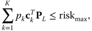
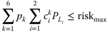
In what follows, the presentation adopts the approach in [27]. This approach uses an overall system risk constraint and expresses the contingency severity in terms of the amount of (prompt) load shedding. The latter is a simple and easy to interpret metric which allows replacing the complexity and accuracy of methods which rely on cascading outages simulation (e.g., [24, 25]), but requires field expertise to set the maximum risk allowed ![]() in (7.39).
in (7.39).
This risk-based OPF (RB-OPF) can be abstractly and generically formulated as follows:
where: ![]() , the new control variable, is the vector of load curtailment in post-contingency states;
, the new control variable, is the vector of load curtailment in post-contingency states; ![]() is the vector of base case load active power;
is the vector of base case load active power; ![]() is the vector of maximum allowed amount of bus load curtailment;
is the vector of maximum allowed amount of bus load curtailment; ![]() is the maximum allowed overall amount of load shedding if a contingency occurs;
is the maximum allowed overall amount of load shedding if a contingency occurs; ![]() is the identity matrix of appropriate dimension;
is the identity matrix of appropriate dimension; ![]() is the probability of contingency
is the probability of contingency ![]() ; and
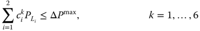
; and ![]() is the maximum value of overall system risk. Constraints (7.36) impose bounds on the percentage of load curtailment; constraints (7.37) impose limits on the allowed amount of load curtailment at any bus; constraints (7.38) model the authorized overall amount of load shedding according to the grid code. The constraint (7.39) enforces that the overall system risk does not exceed a pre-defined value
is the maximum value of overall system risk. Constraints (7.36) impose bounds on the percentage of load curtailment; constraints (7.37) impose limits on the allowed amount of load curtailment at any bus; constraints (7.38) model the authorized overall amount of load shedding according to the grid code. The constraint (7.39) enforces that the overall system risk does not exceed a pre-defined value ![]() . Note that if the transmission system operator does not wish to take any operational risk (i.e., imposing
. Note that if the transmission system operator does not wish to take any operational risk (i.e., imposing ![]() ), this leads to recovery of the traditional OPF problem in the “also corrective” mode [9].
), this leads to recovery of the traditional OPF problem in the “also corrective” mode [9].
7.3.3 Illustrative Example
The main features of the RB-OPF formulation are illustrated using the 5-bus system in Figure 7.1.
7.3.3.1 Detailed Formulation of the RB-OPF Problem
The compact RB-OPF formulation (7.30)–(7.39) is detailed hereafter for the 5-bus system for preventive mode operation.
The objective function (7.30) is the economic dispatch (7.20).
The set of constraints specific to RB-OPF (7.36)–(7.39) take on the form:
Active and reactive power flow equations (7.21), (7.22), at each bus (![]() ) and each system state (
) and each system state (![]() ), are slightly altered to take into account the new load curtailment control variables
), are slightly altered to take into account the new load curtailment control variables ![]() :
:
In terms of inequality constraints, the RB-OPF includes the set of constraints (7.23)–(7.27) as the deterministic OPF.
Finally, the constraints specific to the preventive mode take on the form:
7.3.3.2 Numerical Results
Two scenarios, called relaxed and constrained, are studied. In both scenarios load shedding is performed under a constant power factor. The relaxed scenario studies the impact of the risk constraint (7.43) only and relaxes constraints (7.41) and (7.42). The constrained scenario considers additionally that load shedding is limited to 10![]() of the initial power in (7.41) and the maximum allowed overall amount of load shed per contingency is set to
of the initial power in (7.41) and the maximum allowed overall amount of load shed per contingency is set to ![]() 200 MW in (7.42). Unless otherwise specified it is assumed that each contingency has probability
200 MW in (7.42). Unless otherwise specified it is assumed that each contingency has probability ![]() .
.
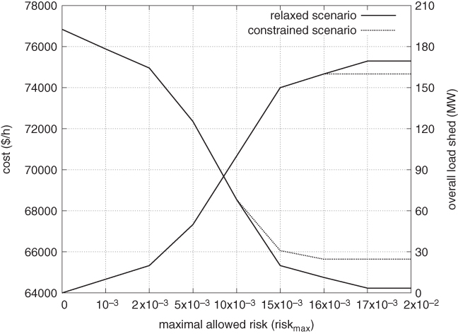
Figure 7.2 Operation cost of RB-SCOPF versus the maximum allowed risk.
Figure 7.2 displays (dotted line) the operation cost obtained with the proposed RB-OPF approach, without short-term constraints, for increasing values of system risk between two extremes: (i) conservative N-1 secure operation which corresponds to ![]() and hence to conventional OPF, as no load shedding is allowed; and (ii) risky N-0 secure operation, where the risk constraint is practically relaxed (e.g., for roughly
and hence to conventional OPF, as no load shedding is allowed; and (ii) risky N-0 secure operation, where the risk constraint is practically relaxed (e.g., for roughly ![]() ). The figure also provides the corresponding overall amount of load shed corresponding to each risk level. One can observe that as the maximum allowed risk increases, the overall load shed increases and the operation cost decreases. This curve could constitute an important basis for a transmission system operator (TSO) to trade-off the cost savings incurred by choosing a more risky operation.
). The figure also provides the corresponding overall amount of load shed corresponding to each risk level. One can observe that as the maximum allowed risk increases, the overall load shed increases and the operation cost decreases. This curve could constitute an important basis for a transmission system operator (TSO) to trade-off the cost savings incurred by choosing a more risky operation.
The potential consequences of the operation risk assumed can be evaluated in terms of post-contingency overall and individual load shedding. These are provided in Table 7.5 for contingency L2, the only contingency that is binding in all cases, as it leads to an active current constraint on line L3. Because the curtailment of load in bus 1 has a larger impact on the loading of critical line L3 (and thereby on the cost reduction), as a consequence, it is fully exploited in all cases, as shown in the table.
Table 7.5 Overall and individual load shedding (MW) for contingency L2
| Relaxed | Constrained | |||||
| Overall | Bus 1 | Bus 2 | Overall | Bus 1 | Bus 2 | |
| 0 | 0.0 | 0.0 | 0.0 | 0.0 | 0.0 | 0.0 |
| 0.001 | 10.0 | 10.0 | 0.0 | 10.0 | 10.0 | 0.0 |
| 0.002 | 20.0 | 20.0 | 0.0 | 20.0 | 20.0 | 0.0 |
| 0.005 | 50.0 | 50.0 | 0.0 | 50.0 | 50.0 | 0.0 |
| 0.010 | 100.0 | 100.0 | 0.0 | 100.0 | 100.0 | 0.0 |
| 0.015 | 150.0 | 150.0 | 0.0 | 150.0 | 110.0 | 40.0 |
| 0.016 | 160.0 | 160.0 | 0.0 | 160.0 | 110.0 | 50.0 |
| 0.017 | 169.4 | 169.4 | 0.0 | 160.0 | 110.0 | 50.0 |
| 0.020 | 169.4 | 169.4 | 0.0 | 160.0 | 110.0 | 50.0 |
7.4 OPF Under Uncertainty
7.4.1 Motivation and Potential Approaches
This section addresses an extended-scope OPF framework that aims to further take into account forecast uncertainty or, in other words, bus power injections uncertainty, stemming mostly from an increasingly significant amount of renewable generation (e.g., wind, solar, etc.). In this increasingly sustainable power systems context, the classical operational planning approach based on the conventional deterministic OPF, which secures only the most likely forecasted state (or nominal scenario) of the system for each period of time of the next day, may be insufficient.
The OPF under uncertainty (OPF-UU) problem can be tackled most notably via approaches from robust optimization [28–31], chance-constrained optimization [32, 33], or stochastic optimization [34]. However, whatever the approach taken, compared to conventional OPF, OPF-UU will need to additionally incorporate a certain number of (base case) aggregated scenarios sampling the uncertainty, which significantly increases the already large problem size.
Assuming that probability density functions of uncertainty are not available or trusted the day ahead of operation, this presentation follows a robust optimization approach. Specifically, a special case of the comprehensive framework proposed in [28] is detailed hereafter.
7.4.2 Robust Optimization Framework
Assume first, without loss of generality, a box uncertainty set ![]() defined by upper and lower bounds on the uncertain power injections, including an infinite number of potential scenarios:
defined by upper and lower bounds on the uncertain power injections, including an infinite number of potential scenarios:
where ![]() is the number of system buses.
is the number of system buses.
The day-ahead robust OPF approach seeks to determine the optimal combination of preventive controls ![]() , which are independent of the power injection pattern, and corrective controls
, which are independent of the power injection pattern, and corrective controls ![]() , which are dependent of both the contingency and the power injection pattern, such that the system operational limits are satisfied whatever postulated contingency
, which are dependent of both the contingency and the power injection pattern, such that the system operational limits are satisfied whatever postulated contingency ![]() and injection scenario
and injection scenario ![]() may show up the next day. This robust OPF (R-OPF) can be abstractly formulated as follows:
may show up the next day. This robust OPF (R-OPF) can be abstractly formulated as follows:
where constraints (7.52)–(7.55) have the same meaning as constraints (7.2)–(7.6) from the conventional OPF formulation, ![]() is a vector of uncertain bus active/reactive power injections, and
is a vector of uncertain bus active/reactive power injections, and ![]() denotes the set of generators that participate in frequency regulation or, in other words, compensate the active power imbalance due to the uncertain power injections. This set of generators is assumed cost-free, according to the objective (7.50), and the nominal scenario corresponds to
denotes the set of generators that participate in frequency regulation or, in other words, compensate the active power imbalance due to the uncertain power injections. This set of generators is assumed cost-free, according to the objective (7.50), and the nominal scenario corresponds to ![]() .
.
By the definition of the set ![]() , the R-OPF problem has an infinite number of constraints. Note that since control variables
, the R-OPF problem has an infinite number of constraints. Note that since control variables ![]() are common to all pre-contingency states, the robust OPF solution (if any) immunizes the power system security against any realization of the uncertainty in the set
are common to all pre-contingency states, the robust OPF solution (if any) immunizes the power system security against any realization of the uncertainty in the set ![]() .
.
7.4.3 Methodology for Solving the R-OPF Problem
The principle of the proposed methodology for solving the R-OPF formulation (7.50)–(7.55) consists of solving a sequence of problem relaxations, by replacing the infinite set of scenarios ![]() with a finite subset of worst-case (or worst uncertainty pattern) scenarios
with a finite subset of worst-case (or worst uncertainty pattern) scenarios ![]() adjusted to the problem instance at hand. The original infinite dimensional problem is thus reduced to a sequence of finite dimensional subproblems. The proposed algorithm builds up iteratively a growing set of constraining scenarios
adjusted to the problem instance at hand. The original infinite dimensional problem is thus reduced to a sequence of finite dimensional subproblems. The proposed algorithm builds up iteratively a growing set of constraining scenarios ![]() as follows:
as follows:
- 1. At the first iteration,
 comprises the nominal scenario
  (i.e., the most likely forecast for the next day), the computation being reduced to a conventional OPF.
 - 2.
Fix
 to the OPF optimum
  derived at the previous step and compute the worst-case scenario with respect to each contingency
  as follows:
- a.
Compute the worst-case scenario
 with respect to contingency
  in the absence of corrective actions by solving the optimization problem:7.57
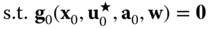 7.58
7.58 7.59
7.59
where
 denotes the subset of violated operation constraints (assumed known beforehand) corresponding to the worst uncertainty pattern. The reader is referred to [30] for an algorithm to identify this subset.
 - b.
If the worst-case scenario leads to constraint violation, check via a special case of OPF if optimal corrective actions are able to remove the constraint violation:
7.62 7.63
7.63 7.64
7.64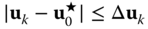
where
 are positive relaxation variables and
  is a large positive penalty term aimed to identify if the original problem is infeasible; otherwise
  .
. - c.
If this is not the case then preventive controls are required to cover the worst-case scenario; grow the subset of worst-case scenarios:
 .
.
- a.
- 3. Compute a new value
 by solving a relaxation of the R-OPF problem (7.50)–(7.55) which includes all scenarios in
  and all contingencies.
 - 4. The process terminates as soon as: (i) a fixed point is reached (i.e., no change in either
 or
or  ), or (ii) computing budget is exhausted, or (iii) the current relaxation of the R-OPF problem (7.50)–(7.55) becomes infeasible (meaning that the best combination of preventive and corrective controls cannot guarantee the system security over the whole uncertainty set
  ). Otherwise, go back to step 2.
Note that this iterative algorithm produces a sequence of day-ahead decisions ![]() of growing robustness with respect to uncertainties since, at any intermediate iteration, besides the nominal scenario, a larger set of uncertain patterns than at the previous iteration are covered.
of growing robustness with respect to uncertainties since, at any intermediate iteration, besides the nominal scenario, a larger set of uncertain patterns than at the previous iteration are covered.
7.4.4 Illustrative Example
A detailed specific formulation of the optimization problems involved in the iterative algorithm for the solution of the R-OPF problem is provided for the 5-bus system.
7.4.4.1 Detailed Formulation of the Worst Uncertainty Pattern Computation With Respect to a Contingency
For simplicity, the worst case scenarios are computed solely with respect to overload and further assume that only one line (known beforehand) is overloaded by the worst uncertainty pattern. The reader is referred to [30] for a detailed comprehensive algorithm to reveal the overall set of overloaded lines whatever the uncertainty pattern and the processing of several overloads in the worst case scenario.
The compact formulation (7.56)–(7.60) is detailed hereafter for contingency ![]() .
.
The objective function is the maximization of the current in the line linking buses ![]() and
and ![]() in the state post-contingency
in the state post-contingency ![]() :
:

The decision variables of this optimization problem are the uncertain power injections (![]() and
and ![]() ), which are allowed to vary in certain ranges:
), which are allowed to vary in certain ranges:
and limits on the active power of the generator responsible for frequency regulation:
The active power and imposed voltage of other generators are fixed, in both states, at the values provided by the conventional OPF (![]() and
and ![]() ):
):
The power flow equations at each bus (![]() ) including uncertain injections for both the base case and the state post-contingency
) including uncertain injections for both the base case and the state post-contingency ![]() (i.e.,
(i.e., ![]() ) are:
) are:

The reference voltage angle constraint is set as:
Operational limits on (longitudinal) branch current, voltage magnitude, and generator reactive power can be written as:
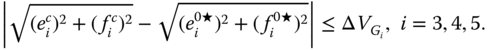
Note that, because the violated line currents in the state post-contingency ![]() are assumed known, other branch current constraints for this state are dropped; hence, constraint (7.74) includes only the set of branch current constraints in the base case.
are assumed known, other branch current constraints for this state are dropped; hence, constraint (7.74) includes only the set of branch current constraints in the base case.
7.4.4.2 Detailed Formulation of the OPF to Check Feasibility in the Presence of Corrective Actions
The compact formulation (7.61)–(7.65) is detailed hereafter for the 5-bus system.
The objective function is the minimization of the amount of generation redispatch, with respect to the values provided by the conventional OPF, to remove violated constraints in the state post-contingency ![]() :
:
The decision variables of this optimization problem are the generators active power and terminal voltage:
The power flow equations at each bus (![]() ) for the state post-contingency
) for the state post-contingency ![]() are:
are:


The reference voltage angle constraint is set as:
Operational limits on (longitudinal) branch current, voltage magnitude, and generator reactive power can be written as:

Finally, the coupling constraints take on the form:
7.4.4.3 Detailed Formulation of the R-OPF Relaxation
A detailed specific formulation of the R-OPF relaxation problem including a finite number of worst case scenarios (![]() ), where
), where ![]() corresponds to the nominal scenario, is provided hereafter.
corresponds to the nominal scenario, is provided hereafter.
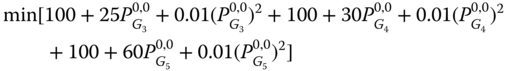
The objective function is economic dispatch (i.e., minimum generation cost):
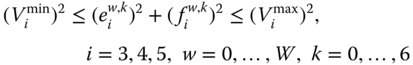
The decision variables of this problem are the generators active power and terminal voltage, which are limited within some ranges:
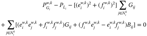
The active and reactive power flow equations at each bus (![]() ) and for each uncertainty scenario (
) and for each uncertainty scenario (![]() ) and system state (
) and system state (![]() ) are:
) are:
The reference voltage angle constraint is:
Operational limits on (longitudinal) branch current, voltage magnitude, and generator reactive power can be written as:

Finally, the coupling constraints (7.55) are:

7.4.4.4 Numerical Results
The main characteristics of the abstract OPF-UU formulation are best shown for educational purposes using the 5-bus system in Figure 7.1.
Uncertainty can be assumed to stem from renewable generation present in lower voltage grids, which have not been explicitly modeled, the renewable generation being simply aggregated to load buses 1 and 2. Uncertainty is modeled as variable active and reactive power injections at the two load buses in the range of −5![]() to +5
to +5![]() of the nominal active/reactive load.
of the nominal active/reactive load.
Following the proposed methodology for solving the R-OPF problem, one first computes a reference schedule for the nominal scenario via classical OPF formulation in “also corrective” mode including the six postulated contingencies (see Table 7.6).
The solution provided by this classical OPF computes, via the formulation (7.66), (7.67), (7.68), (7.69), (7.70), (7.71), (7.72), (7.73), (7.74), (7.75), (7.76), the worst uncertainty pattern for each contingency with respect to thermal overload. Note that, due to the network simplicity, only one worst uncertainty pattern, common for all contingencies, is revealed. The worst uncertainty pattern corresponds to a case where the output of renewable generation at buses 1 and 2 is zero. Accordingly, the pre-contingency state corresponding to the worst uncertainty pattern differs, with respect to the classical OPF solution, by additional active/reactive power drawn from the network (i.e., 55 MW/20 MVAr at bus 1 and 25 MW/10 MVAr at bus 2, respectively), the active power balance being ensured by an increase of 83.3 MW at G5, while the generators' reactive power production change so as to maintain their imposed voltages in the prevailing operation conditions.
Further, only two out of six contingencies lead to overloads for their worst uncertainty pattern. Specifically, contingency L2 overloads line L3 with 0.95 pu and contingency L4 also overloads line L3 with 0.9 pu. In both cases, upon solving the formulation (7.77), (7.78), (7.79), (7.80), (7.81), (7.82), (7.83), (7.84), (7.85), (7.86), one observes that the overload cannot be fully removed despite the best use of corrective actions. Specifically, for contingency L2, the best redispatch scheme consists in reducing the active power of G4 and increasing the active power of G5, which creates a counterflow in the overloaded line L3. The latter line current cannot be reduced to more than 11.53 pu. For contingency L4, despite the best redispatch between generators G3 and G4 (where the former increases its production), which creates a counterflow in the overloaded line L3, its latter current is reduced only to 11.12 pu.
Next, in order to compute the intermediate robust optimal solution, one solves the R-OPF formulation (7.87), (7.88), (7.89), (7.90), (7.91), (7.92), (7.93), (7.94), (7.95), (7.96) which includes the reference scenario and the sole worst case scenario found (common to both contingencies).
Table 7.6 provides, for various operating modes, the values of the objective, the six decision variables, and the binding operation constraints. Note that the robust optimal solution encompasses both the active power and the terminal voltage of each generator.
In the second loop of the algorithm, one notices that the worst uncertainty pattern does not change. Because the latter scenario is already covered by the R-OPF solution, this means that the algorithm reaches a fixed point and hence this schedule is the robust optimal solution. The operation cost of robustness exceeds roughly 10% the cost of the most likely scenario (see Table 7.6).
Table 7.6 Values of the objective, decision variables, and critical post-contingency constraints for various operating modes
| Objective | Decision variables | Critical constraints | |||||||
| Operating | cost | ||||||||
| modes | MW | MW | MW | pu | pu | pu | pu | pu | |
| also corrective | 70550 | 668.2 | 442.7 | 519.1 | 1.050 | 1.050 | 1.050 | 10.8 | 11.0 |
| robust solution | 77235 | 700.5 | 228.7 | 703.2 | 1.050 | 1.047 | 1.050 | 10.5 | 10.8 |
7.5 Advanced Issues and Outlook
7.5.1 Conventional OPF
7.5.1.1 Overall OPF Solution Methodology
In order to facilitate the understanding of the major basic concepts of an OPF problem, the latter has been assumed as a clean mathematical programming problem (e.g., NLP) which can be solved directly by an appropriate optimization method (e.g., IPM). However, real-world OPF problems are far more complex. For instance, the major challenges to today's deterministic OPF problems are [2–6]: (i) the huge size, (ii) the management of discrete control variables, and (iii) the incorporation of several problem peculiarities that reflect TSO practical needs (e.g., usable solution in terms of number and sequence of corrective actions, etc.) and operating rules (e.g., conditional corrective actions, constraints and control variables priorities, etc.). Regarding item (iii), it must be emphasized that some practical aspects of the OPF problem may not be formulated analytically in an advantageous form exploitable by an optimizer, requiring one to resort to heuristic techniques during the OPF solution methodologies [2]. However, since benchmarks of practical real-world OPF problems are not available,8 the academic realm typically only addresses items (i) and (ii), interpreting, in the most ambitious vision, a real-life OPF problem as a large scale non-convex mixed-integer nonlinear programming (MINLP) problem [22].
The huge size of real-life OPF problems stems from the large number of contingencies that have to be secured (e.g., at least all N-1 events) and the large size of the power system. Because taking a direct approach to such a problem is computationally inefficient if even feasible, methodologies for solving practical OPF problems require decomposition into (and iterations over) a certain number of modules (see Figure 7.3) including in the most generic also corrective mode:
- Core NLP optimizers for the master problem and slave (i.e., contingency) problems: The master problem includes constraints for the base case and some potentially binding contingencies while each slave problem relates to a post-contingency state and checks whether it is feasible thanks to corrective actions.
- Manager of discrete variables module: sets discrete control variables according to some approach (e.g., round-off [36], progressive round-off [22, 37], sensitivity-based [38]) or dedicated techniques for topology control (transmission switching) [39]. Note that this module may interact several times during the solution process with optimizers for both master and slave problems.
- Security analysis module: performs classical post-contingency power flow calculations to check whether constraints violations occur.
- Contingency selection (or filtering) module: selects from the set of contingencies that violate constraints some promising potentially binding contingencies to be added to the master optimizer [20, 21, 40, 41].
An acceptable solution of the OPF problem is found (and iterations stop) when no contingency leads to constraint violation in the presence of corrective actions.
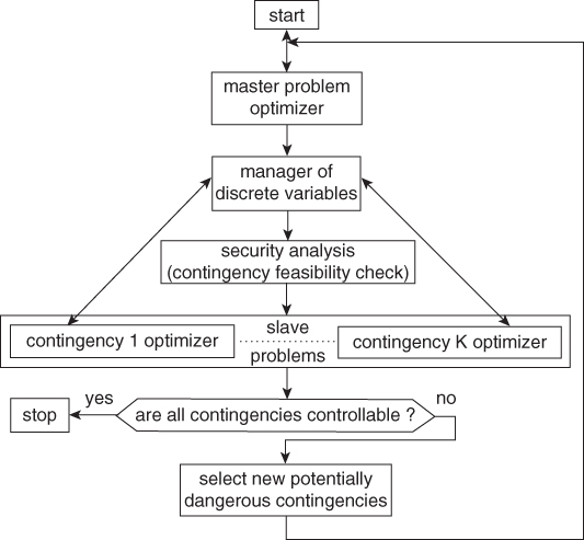
Figure 7.3 High level flowchart of the OPF solution methodology in the also corrective mode.
Significant progress in the OPF state-of-the-art has been achieved recently in the following methodologies for problem decomposition: all potentially binding contingencies together (possibly with post-contingency network compression) [20–22]; adaptive Benders decomposition [42] (which improves solution quality but requires larger computational effort compared to the classical Benders decomposition-based OPF methodology [9, 21]); and alternating direction method of multipliers [42]. The core optimizer in these methodologies utilizes powerful general-purpose local solvers (mostly based on the IPM) for NLP (e.g KNITRO and IPOPT). The use of high performance computations renders these computationally demanding OPF methodologies practical for solving realistic large-scale OPF problems (e.g., for large systems up to roughly 10 000 buses and 12 000 contingencies [22]), even starting “from scratch.” Because the core optimizer in these methodologies is the IPM, further improvement can be obtained by decomposing the structure of the linear system of equations to be solved in the interior point method [40]. Anyway, to cope with stringent OPF running time industry needs, powerful computing infrastructure is deployed enabling distributed (parallel) computations and hence fostering OPF decomposition methods.
7.5.1.2 Core Optimizers: Classical Methods Versus Convex Relaxations
In most today OPF commercial software used by the industry, the core optimizer relies on SLP, SQP, Newton's method, and IPM. Although solvers for LP and QP are reliable and fast, SLP and SQP methodologies may provide approximate solutions of the NLP core problem, especially for highly nonlinear OPF problems (e.g., reactive power dispatch). Newton's method and IPM can provide exact (at least) local optimum for the underlying NLP core problem, but while Newton's method may have difficulties in handling inequality constraints, IPM (both general-purpose and produced by academia, tailored specifically for the OPF problem) is not fully reliable [17] and does not warm/hot start well. The warm/hot start feature of an algorithm (via the latest solution at hand or an intermediate approximated solution at a given iteration) is supposed to generally accelerate OPF solution methodologies, especially if successive master problem solutions are close to each other, or their active set of constraints do not change significantly.
A research framework that has attracted much interest recently is devoted to convex relaxations9 of the non-convex NLP problems intervening in the core optimizers [44–46]. The major goal of these approaches is to provide, in certain conditions, the global optimum of the non-convex NLP continuous relaxation of the OPF problem. Other notable advantages of these approaches are: provision of a lower bound of the NLP problem (which allows evaluation, provided that the relaxation is tight, of the quality of the local optimizer solution), problem infeasibility guarantee, reliability, and polynomial solution time. Most of these approaches rely on either semi-definite programming (SDP) relaxation [44] or the more general high-order moment-based relaxation [45] (in fact SDP relaxation corresponds to the first order moment).
Various research with convex relaxations report very useful empirical evidence that, generally, the solution provided by local optimizers is the global optimum (or a solution of very high quality) [42, 45, 46]. Next, extensive experiments conducted using a diverse data set point out that [46]: (i) in most cases SDP relaxation does not recover the global solution (since the duality gap is greater than 0%) and (ii) convex relaxations methods are generally slower and scale less well than local optimizers on large OPF problems. Further research with convex relaxations is therefore needed in order to reduce the computational burden, improve the convergence precision of SDP [45], solve real-life OPF problems (which, inter alia, may present negative Lagrange multipliers), and so on.
“It is important to emphasize that, due to today's limitations of the MINLP state-of-the-art, when solving real-life large-scale AC OPF problems under stringent time requirements, the aspect of whether the solution of the OPF continuous relaxation dealt with by the core optimizer is the global optimum or not becomes definitely of secondary importance compared to the primary aim which is to provide, within the allowed computational budget, a (possibly sub-optimal) solution which satisfies the constraints.” [6]. Furthermore, it is worth mentioning that the core algorithm classification (approximate, at least local, or global) relates to the ideal case of a perfect system state forecast, which is less and less the case in today's increasingly uncertain operational environment (especially in day-ahead, which has been the main OPF application timeframe).
Although there is definitely room to improve convex relaxations in the coming years and even make them usable by industry as a complement for classical well-established non-convex local optimizers (in terms of solution quality and certificate of problem infeasibility), it is unlikely that these relaxations will eventually supersede local optimizers.
Finally, in order to efficiently solve increasingly complex practical OPF problems, there will be no single winner in terms of method adopted by the core optimizer, but rather modern optimizers will embed different solution methods (like the powerful solver KNITRO), being able to seamlessly switch between them in order to adapt on-the-fly to the features of the optimization problem at hand.
7.5.2 Beyond the Scope of Conventional OPF: Risk, Uncertainty, Smarter Sustainable Grid
Driven by stringent sustainability commitments, the fast-paced integration of a significant amount of intermittent renewable generation at all voltage levels requires smarter operation of the grid. The latter can be achieved first of all through the provision and smart management of operation flexibility, which enables the system to maintain security while adapting to unforeseen prevailing operational conditions. This increases the reliance upon effective controllable devices (e.g., phase shifters, storage, FACTS devices, HVDC links, topology control, etc.) as fast corrective actions for controlling both post-contingency and poorly predicted operation conditions. As a consequence, the decision making process close to and in real-time will gain more attention and utilization. This calls for faster OPF solution methodologies, possibly different to those developed for the main (day-ahead) OPF purpose, tailored for closer to real-time application.
Furthermore, such smarter operation of increasingly sustainable power systems will require in turn a flexible decision making process balancing risk-based security criteria and renewable generation forecast uncertainty. This very ambitious goal will lead in the future to the development of the first generation of risk-based AC OPF under uncertainty tools. This highly complex and computationally challenging problem is today out of reach using the AC grid model. For instance, [34] provides the most computationally advanced risk-based OPF under uncertainty tool in terms of optimization problem features (e.g., a few hundred thousand variables and constraints are considered). However, this work adopts the DC approximation, highlighting the immense computational challenge (and hence tool capability limitations) of handling simultaneously multiple periods, contingencies, uncertain power injections scenarios, many binary variables, and so on. There is therefore an enormous research potential in this area for developing not only frameworks [33, 34, 47] but, more importantly, scalable algorithms. Specifically, in lieu of tackling this highly complex paradigm directly, there is a need to properly address both its sub-fields, that is, risk-based OPF and OPF under uncertainty, while improving the algorithms of the deterministic AC OPF framework, which can yield efficient common building blocks. In terms of large scale application, both sub-fields are still insufficiently mature, unless one adopts a DC-based approach that has proven scalability to large systems [26, 29]. “However, this paper argues that scalable methodologies for deterministic AC OPF can be adapted to risk-based AC OPF problems, providing that the latter are formulated in a decomposable way, fostering the leverage of RB-OPF to large scale systems. As regards AC OPF under uncertainty, although some promising results have been obtained within the robust optimization framework for a medium size system [28], such an approach remains very computationally heavy” [6]. In order to provide more tractable algorithms, the major focus should be devoted to the reduction of the number of critical scenarios modeling the uncertainty (e.g., through efficient scenario aggregation), which is responsible for the most additional computational burden compared to deterministic OPF.
The time line of decision making should be revisited depending on the degree of trust in available uncertainty models. Thus, one can envision favoring robust optimization in day-ahead applications, chance constrained or stochastic optimization in intraday, and deterministic optimization close to real-time.
Another research line beyond the scope of deterministic OPF consists in seeking for optimal solutions while additionally taking into account (voltage, transient, and small-disturbance) stability constraints via either deriving approximations of the stability boundaries and including them directly into the OPF or coupling OPF and time-domain simulation [48–50]. This is a very important extension of the OPF scope but remains with a high computational burden for which scalable approaches of reasonable accuracy need to be found.
Another essential group of additional control options to be investigated are demand response management techniques, which offer additional degrees of freedom in terms of load shifting and large scale deployment of storage devices, for which fast technological progress is envisioned. These new control means will require optimization to be performed on a longer time horizon leading to consideration of multi-period OPF applications.
Finally, attention should also be paid to the interface with distribution grids, which are increasingly active in terms of distributed generation and may offer useful ancillary services in the future.
References
- 1 Jacques, C. (1962) Contribution à l'étude du dispatching économique, in Bulletin de la Societé Française d'Electricité, vol. 3, pp. 431–447.
- 2 Stott, B. and Alsac, O. (2012) Optimal power flow - basic requirements for real-life problems and their solutions (white paper), in SEPOPE XII Symposium, Rio de Janeiro, Brazil.
- 3 Capitanescu, F., Martinez Ramos, J.L., Panciatici, P., Kirschen, D., Marano Marcolini, A., Platbrood, L., and Wehenkel, L. (2011) State-of-the-art, challenges, and future trends in security constrained optimal power flow. Elec. Pow. Syst. Research, 81 (8), 1731–1741.
- 4 Momoh, J., Koessler, R., Bond, M., Stott, B., Sun, D., Papalexopoulos, A., and Ristanovic, P. (1997) Challenges to optimal power flow. Power Systems, IEEE Transactions on, 12 (1), 444–455.
- 5 Stott, B., Alsac, O., and Monticelli, A.J. (1987) Security analysis and optimization. Proceedings of the IEEE, 75 (12), 1623–1644.
- 6 Capitanescu, F. (2016) Critical review of recent advances and further developments needed in AC optimal power flow. Elec. Pow. Syst. Research, 136, 57–68.
- 7 Overbye, T.J., Cheng, X., and Sun, Y. (2004) A comparison of the AC and DC power flow models for LMP calculations, in System Sciences, 2004. Proceedings of the 37th Annual Hawaii International Conference on, IEEE.
- 8 Alsac, O. and Stott, B. (1974) Optimal load flow with steady-state security. Power Apparatus and Systems, IEEE Transactions on, 93 (3), 745–751.
- 9 Monticelli, A.J., Pereira, M.V.P., and Granville, S. (1987) Security-constrained optimal power flow with post-contingency corrective rescheduling. Power Systems, IEEE Transactions on, 2 (1), 175–182.
- 10 Alsac, O., Bright, J., Prais, M., and Stott, B. (1990) Further developments in LP-based optimal power flow. Power Systems, IEEE Transactions on, 5 (3), 697–711.
- 11 Burchett, R., Happ, H., and Vierath, D. (1984) Quadratically convergent optimal power flow. Power Apparatus and Systems, IEEE Transactions on, 103 (11), 3267–3275.
- 12 Sun, D.I., Ashley, B., Brewer, B., Hughes, A., and Tinney, W.F. (1984) Optimal power flow by Newton approach. Power Apparatus and Systems, IEEE Transactions on, 103 (10), 2864–2880.
- 13 Wu, Y.C., Debs, A.S., and Marsten, R.E. (1994) A direct nonlinear predictor-corrector primal-dual interior point algorithm for optimal power flows. IEEE Trans. Power Syst., 9 (2), 876–883.
- 14 Granville, S. (1994) Optimal reactive dispatch through interior point methods. IEEE Trans. Power Syst., 9 (1), 136–146.
- 15 Torres, G.L. and Quintana, V.H. (1998) An interior-point method for nonlinear optimal power flow using rectangular coordinates. IEEE Trans. Power Syst., 13 (4), 1211–1218.
- 16 Torres, G.L. and Quintana, V.H. (2001) On a nonlinear multiple-centrality-corrections interior-point method for optimal power flow. IEEE Trans. Power Syst., 16 (2), 222–228.
- 17 Capitanescu, F. and Wehenkel, L. (2013) Experiments with the interior-point method for solving large scale optimal power flow problems. Elec. Pow. Syst. Research, 95 (2), 276–283.
- 18 Fiacco, A.V. and McCormick, G.P. (1968) Nonlinear programming: Sequential unconstrained minimization techniques, in John Willey & Sons.
- 19 Martinez Ramos, J.L. and Quintana, V.H. (2009) Optimal and secure operation of transmission systems. Electric Energy Systems: Analysis and Operation, CRC Press, Boca Raton, pp. 211–264.
- 20 Capitanescu, F., Glavic, M., Ernst, D., and Wehenkel, L. (2007) Contingency filtering techniques for preventive security-constrained optimal power flow. Power Systems, IEEE Transactions on, 22 (4), 1690–1697.
- 21 Capitanescu, F. and Wehenkel, L. (2008) A new iterative approach to the corrective security-constrained optimal power flow problem. Power Systems, IEEE Transactions on, 23 (4), 1533–1541.
- 22 Platbrood, L., Capitanescu, F., Merckx, C., Crisciu, H., and Wehenkel, L. (2014) A generic approach for solving nonlinear-discrete security-constrained optimal power flow problems in large-scale systems. Power Systems, IEEE Transactions on, 29 (3), 1194–1203.
- 23 Condren, J., Gedra, T.W., and Damrongkulkamjorn, P. (2006) Optimal power flow with expected security costs. Power Systems, IEEE Transactions on, 21 (2), 541–547.
- 24 He, J., Cheng, L., Kirschen, D.S., and Sun, Y. (2010) Optimising the balance between security and economy on a probabilistic basis. IET Gener. Transm. Distrib., 4 (12), 1275–1287.
- 25 Karangelos, E., Panciatici, P., and Wehenkel, L. (2013) Whither probabilistic security management for real-time operation of power systems ?, in IREP Symposium - Bulk Power Systems Dynamics and Control-IX (IREP), Rethymnon, Greece.
- 26 Wang, Q., McCalley, J.D., Zheng, T., and Litvinov, E. (2016) Solving corrective risk-based security-constrained optimal power flow with lagrangian relaxation and benders decomposition. International Journal of Electrical Power & Energy Systems, 75 (2), 255–264.
- 27 Capitanescu, F. (2015) Enhanced risk-based scopf formulation balancing operation cost and expected voluntary load shedding. Elec. Pow. Syst. Research, 128 (1), 151–155.
- 28 Capitanescu, F., Fliscounakis, S., Panciatici, P., and Wehenkel, L. (2012) Cautious operation planning under uncertainties. Power Systems, IEEE Transactions on, 27 (4), 1859–1869.
- 29 Fliscounakis, S., Panciatici, P., Capitanescu, F., and Wehenkel, L. (2013) Contingency ranking with respect to overloads in very large power systems taking into account uncertainty, preventive, and corrective actions. Power Systems, IEEE Transactions on, 28 (4), 4909–4917.
- 30 Capitanescu, F. and Wehenkel, L. (2013) Computation of worst operation scenarios under uncertainty for static security management. Power Systems, IEEE Transactions on, 28 (2), 1697–1705.
- 31 Korad, A. and Hedman, K. (2013) Robust corrective topology control for system reliability. Power Systems, IEEE Transactions on, 28 (4), 4042–4051.
- 32 Roald, L., Vrakopoulou, M., Oldewurtel, F., and Andersson, G. (2015) Risk-based optimal power flow with probabilistic guarantees. International Journal of Electrical Power & Energy Systems, 72, 66–74.
- 33 Hamon, C., Perninge, M., and Söder, L. (2015) A computational framework for risk-based power systems operations under uncertainty. part I: Theory. Electric Power Systems Research, 119, 45–53.
- 34 Murillo-Sanchez, C., Zimmerman, R., Lindsay Anderson, C., and Thomas, R. (2013) Secure planning and operations of systems with stochastic sources, energy storage and active demand. Smart Grid, IEEE Transactions on, 4 (4), 2220–2229.
- 35 Zimmerman, R., Murillo-Sanchez, C., and Thomas, R. (2011) MATPOWER: Steady-state operations, planning and analysis tools for power systems research and education. Power Systems, IEEE Transactions on, 26 (1), 12–19.
- 36 Papalexopoulos, A., Imparato, C., and Wu, F. (1989) Large-scale optimal power flow: Effects of initialization, decoupling & discretization. Power Systems, IEEE Transactions on, 4, 748–759.
- 37 Macfie, P., Taylor, G., Irving, M., Hurlock, P., and Wan, H. (2010) Proposed shunt rounding technique for large-scale security constrained loss minimization. Power Systems, IEEE Transactions on, 25 (3), 1478–1485.
- 38 Capitanescu, F. and Wehenkel, L. (2010) Sensitivity-based approaches for handling discrete variables in optimal power flow computations. Power Systems, IEEE Transactions on, 25 (4), 1780–1789.
- 39 Rolim, J. and Machado, L. (1999) A study of the use of corrective switching in transmission systems. Power Systems, IEEE Transactions on, 14 (1), 336–341.
- 40 Jiang, Q. and Xu, K. (2014) A novel iterative contingency filtering approach to corrective security-constrained optimal power flow. Power Systems, IEEE Transactions on, 29 (3), 1099–1109.
- 41 Ardakani, A.J. and Bouffard, F. (2013) Identification of umbrella constraints in dc-based security-constrained optimal power flow. Power Systems, IEEE Transactions on, 28 (4), 3924–3934.
- 42 Phan, D. and Kalagnanam, J. (2014) Some efficient methods for solving the security-constrained optimal power flow problem. Power Systems, IEEE Transactions on, 29 (2), 863–872.
- 43 Panciatici, P., Campi, M., Garatti, S., Low, S., Molzahn, D., Sun, A., and Wehenkel, L. (2014) Advanced optimization methods for power systems, in Power Systems Computation Conference (PSCC), 2014, IEEE, pp. 1–18.
- 44 Lavaei, J. and Low, S. (2012) Zero duality gap in optimal power flow problem. Power Systems, IEEE Transactions on, 27 (1), 92–107.
- 45 Molzahn, D.K. and Hiskens, I.A. (2015) Sparsity-exploiting moment-based relaxations of the optimal power flow problem. Power Systems, IEEE Transactions on, 30 (6), 3168–3180.
- 46 Coffrin, C., Hijazi, H., and Van Hentenryck, P. (2016) The QC relaxation: A theoretical and computational study on optimal power flow. Power Systems, IEEE Transactions on.
- 47 Varaiya, P.P., Wu, F.F., and Bialek, J.W. (2011) Smart operation of smart grid: risk-limiting dispatch. Proceedings of the IEEE, 99 (1), 40–57.
- 48 Bruno, S., De Tuglie, E., and La Scala, M. (2002) Transient security dispatch for the concurrent optimization of plural postulated contingencies. Power Systems, IEEE Transactions on, 17 (3), 707–714.
- 49 Capitanescu, F., Van Cutsem, T., and Wehenkel, L. (2009) Coupling optimization and dynamic simulation for preventive-corrective control of voltage instability. Power Systems, IEEE Transactions on, 24 (2), 796–805.
- 50 Hamon, C., Perninge, M., and Soder, L. (2013) A stochastic optimal power flow problem with stability constraints - part I: Approximating the stability boundary. Power Systems, IEEE Transactions on, 28 (2), 1839–1848.