
Chapter 17
High-Speed Transmission Line Protection Based on Empirical Orthogonal Functions
Rommel P. Aguilar1 and Fabián E. Pérez-Yauli2
1Institute of Electrical Energy, Universidad Nacional de San Juan, Argentina
2Department of Electrical Energy, Escuela Politécnica Nacional, Quito, Ecuador
17.1 Introduction
In order to provide an economical and efficient power supply, bulk power exchange between remote locations is essential. Thus, power transmission at extra-high voltage (EHV) levels is a common practice nowadays. However, as with any part of the power system, the elements that constitute the EHV transmission system are exposed to a number of factors that can cause critical faults. In fact, abnormalities introduced during fault events in EHV networks can not only produce catastrophic damage in the equipment but also lead the entire power system into unstable operation. Additionally, in spite of continuously growing energy demand, factors like de-regulated market, economics, rights-of-way, and environmental restrictions have limited the building of new transmission lines. As a result, existing transmission lines are forced to operate at high loadings, close to their operating limits. Consequently, it is imperative to develop protection devices as well as protection schemes with high-speed performance, which decrease the effect of faults on power system operation and also become an economic way to increase power transfer in a network without investment in new transmission lines.
Over the last three decades, a lot of research has been conducted in the development of ultra-high-speed protection algorithms. Particularly in the late 1970s and '80s, a number of researchers presented significant advances in this area. However, the available technology at that time was not adequate for the high computation requirements of such protection schemes, and therefore they could not take advantage of sophisticated techniques for transient analysis.
Despite the important technological advances in microprocessor based relays, the basic principle of transmission line protection has not changed for more than half a century [1]. This principle is based on extracting the power frequency components of current and voltage signals by means of so-called phasor estimation techniques [2]. These techniques use analog and digital filtering to attenuate the non-power frequency signals caused by fault generated transients and extract only information concerning the power frequency component. Thus, the success of phasor estimation techniques depends on how well the non-power frequency components are filtered out. However, in certain applications, particularly in EHV and ultra-high voltage (UHV) transmission lines, fault signals are prone to be highly contaminated with non-power frequency transients. Thus, the accuracy of phasor estimation is reduced [1, 3]. In fact, these algorithms suffer not only from accuracy problems but also from unwanted responses, noise, disturbance rejections, and reliability issues [3]. Additionally, the filtering process involves an inherent delay that limits the operation time to at least the length of the time window of the filter (normally one cycle of the fundamental frequency for phasor estimation techniques).
A solution to improving the operation time of transmission line protection is reducing the relay data window. However, for data windows shorter than one cycle, information on the steady-state power frequency component decreases whereas the transient content becomes more important. These shortcomings suggest that, for developing faster protection schemes, the analysis must be done over the entire frequency spectrum contained in electrical signals [4]. Therefore, identification of complex waveforms is required instead of the evaluation of periodic characteristics [1]. In this field, the term Transient Based Protection appears, which is based on analysis of the entire frequency spectrum contained in transient current and voltage signals appearing after a fault. This principle proposes that high frequency components contained in transient signals provide valuable information for achieving fast and accurate protection [4, 5].
The development of Electromagnetic Transients Programs (EMTP) and real-time digital simulators [6] established the fundamental basis for modeling and analysis of power system transients. In this field, more accurate models have been introduced over the years to represent the complexities of power systems. In fact, nowadays one can affirm with certainty that simulations using EMTP provide a faithful replica of real power systems. Therefore, these simulations allow gathering a (theoretically) infinite number of observations from a modeled power system. In this context, data mining and signal processing tools play an important role, since they allow relevant information to be obtained from simulation-generated data in order to achieve a meaningful understanding of the real phenomena.
It is well known that faults appear in a stochastic manner. Hence, for a power system exposed to a number of external factors, it is almost impossible to predict when, where, and how a fault will arise. However, despite the innumerable variables that influence the features of a fault, all the faults that can take place in a transmission line have the same mean where they appear and propagate, and then they share a common characteristic. Therefore, the patterns that govern fault generated transients help us to develop protection algorithms, based on the knowledge acquired from data mining and signal processing of a representative sample of fault generated transients.
In this context, the data mining technique known as Empirical Orthogonal Functions (a.k.a. Principal Components Analysis) emerges as a powerful tool for power system applications [7–11]. This technique is used to find a small set of orthogonal functions that gives a good interpretation concerning fault generated transients. Results show that fault signals decomposed in terms of these orthogonal basis functions exhibit well-defined patterns, which can be used for recognizing the main features of fault events such as inception angle, fault type, and fault location. Signals of less than a quarter of cycle can be used, hence high-speed protection algorithms can be designed utilizing these orthogonal basis functions.
The organization of this chapter is as follows: Section 17.2 introduces the theoretical background of Empirical Orthogonal Decomposition. Next, applications of Empirical Orthogonal Functions for transmission line protection are provided in Section 17.3. A case study and evaluation of the protection scheme is presented in 17.4. Finally, conclusions are drawn in Section 17.5.
17.2 Empirical Orthogonal Functions
The term Empirical Orthogonal Functions (EOFs) was first mentioned by Edward Lorenz in 1956 as mechanism to find a simplified but optimal representation of climate data with time and space dependence [12]. Subsequently, this technique has been widely employed in oceanography and meteorology for data compression and pattern extraction [13, 14]. Contrary to other feature extraction techniques that employ exhaustive supervised training, EOFs are easy to implement and do not require adjustment of control parameters. They depend solely on the nature of the input data.
In scientific literature, the EOF technique is also referred to as Principal Components Analysis (PCA) [15–19]. Actually both techniques, EOFs and PCA, are the same. However, for signal processing, the term EOF is more appropriate than PCA, because the term EOF and the theory behind it were founded on the analysis of time series structures. EOFs allows decomposition of a signal in terms of orthogonal basis functions that give an optimal representation of the data. Therefore, it leads to a better understanding of the signal structure.
17.2.1 Formulation
Let the vector ![]() be a time series representing a p-length data window captured from the ith discrete signal of a set of n measured signals. Then this set of signals can be represented by the n×p data matrix X:
be a time series representing a p-length data window captured from the ith discrete signal of a set of n measured signals. Then this set of signals can be represented by the n×p data matrix X:
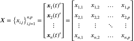
where n is the number of observed signals and p is the number of samples per signal.
For signal analysis it will be further assumed that each discrete signal (time series) is an observation, and each sample is a feature. The element xi,j is a generic element of X, which represents the value of the feature j in the observation i.
EOFs are based on the assumption that any observation xi(t) can be expanded in terms of orthogonal basis functions so that:
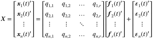
where f1(t), f2(t),…, fp(t) are the orthogonal basis functions, which are called the EOFs, and qij is the decomposition coefficient of xi(t) on fj(t). The number of EOFs is equal to the number of features (p), thus (17.2) expands xi(t) without loss of information [20]. However, p could be a large number; then for dimensionality reduction, it is desirable to select a small number of EOFs. Therefore, the series is truncated as follows:
Here, ![]() is the error associated with the truncation, and r is the number of selected EOFs,
is the error associated with the truncation, and r is the number of selected EOFs, ![]() . In matrix form, (17.3) gives:
. In matrix form, (17.3) gives:
where ![]() contains the coefficients qij for i=1,2,…n, and j=1,2,…r;
contains the coefficients qij for i=1,2,…n, and j=1,2,…r; ![]() is the matrix containing in its columns the r-EOFs [ f1(t), f2(t), …, fr(t)]; and
is the matrix containing in its columns the r-EOFs [ f1(t), f2(t), …, fr(t)]; and ![]() contains in its rows the decomposition errors [ϵ1(t), ϵ2(t), …, ϵn(t)]′. The detailed expression for (17.4) is then:
contains in its rows the decomposition errors [ϵ1(t), ϵ2(t), …, ϵn(t)]′. The detailed expression for (17.4) is then:
where the decomposition errors are formed by the truncated orthogonal basis functions ![]() :
:
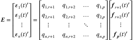
From the above equation, it can be demonstrated that ![]() (n×r matrix of zeros), because of the fact that
(n×r matrix of zeros), because of the fact that ![]() for
for ![]() (definition of orthogonality). Additionally, without loss of generality it can be assumed that any orthogonal function fj(t) has norm 1, which means that
(definition of orthogonality). Additionally, without loss of generality it can be assumed that any orthogonal function fj(t) has norm 1, which means that ![]() (r×r identity matrix). Therefore, the decomposition coefficients are obtained by:
(r×r identity matrix). Therefore, the decomposition coefficients are obtained by:
That is:
It is desirable to find a set of r-EOFs that retain as much as possible of the information of X. That is, E in (17.4) has to be minimized. The solution to the problem states that EOFs are obtained by:
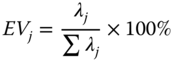
Each eigenvector fj(t) has an associated eigenvalue λj, which represents the amount of information that fj(t) retains from X after the decomposition. Thus, those eigenvectors with higher associated eigenvalue acquire more information from input data. The term explained variability (EV) is used as a measure of the amount of information retained by each EOF.
The order of the EOFs is defined in accordance to their explained variability. That is, the first of the EOFs is the one having the greatest associated eigenvalue.
17.3 Applications of EOFs for Transmission Line Protection
Based on the characteristics and patterns of fault generated transients, this section introduces the proposed protection algorithms. Figure 17.1 presents the general protection scheme: the first stage consists of the formulation of the EOFs, which is the basis for pattern extraction of fault generated transients affecting the protected transmission line. This process is done offline and requires modeling of the protected transmission line and associated power system. Fault simulation is then performed to obtain a fault database, which is then used for attaining the EOF and the associated scores X(q) that represent the fault database in the EOF domain.
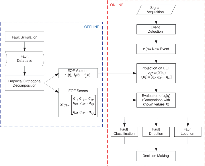
Figure 17.1 Proposed algorithm, general scheme.
The online algorithm begins with signal acquisition that consists of measuring of analog signals from the transducer and transformation to digital signals through an A/D converter. An algorithm is then implemented for event detection: once a potential fault is detected, the wavefront of this event is extracted from the signal; this wavefront must have the same sampling frequency and number of samples as the stated EOF. The detected event defined by the discrete signal x(t) is then decomposed with the selected EOF, which gives a set of values that define the event in the EOF domain x(q). This signal is then compared with precomputed faults that serve as reference for implementation of protection functions. Finally, the protection scheme has to decide which action should be executed.
17.3.1 Fault Direction
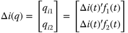
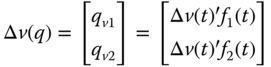
When the power system is not radial, faults can be fed by both line ends. Then defining the fault direction is indispensable for adequate fault location and guaranteeing selectivity in power system protection. For this protection function, decomposition using the two first EOFs is used; that is, fault current and voltage signals are represented by:
The directional function requires comparison of ![]() and
and ![]() , then f1(t) and f2(t) obtained for forward fault currents are used. This is not a general rule—EOFs obtained from voltage signals can also be used and the results are similar.
, then f1(t) and f2(t) obtained for forward fault currents are used. This is not a general rule—EOFs obtained from voltage signals can also be used and the results are similar.
The general scheme for directional evaluation is presented in Figure 17.2. After a fault is detected, the relay extracts the superimposed quantities of current and voltage signals sampled with the same data window and sampling frequency used for obtaining f1(t) and f2(t). Then, both discrete signals are decomposed with f1(t) and f2(t), which results in:
The angle between current and voltage vectors in the EOF space is given by:

Where ![]() and
and ![]() are the norm of
are the norm of ![]() and
and ![]() , respectively, and
, respectively, and ![]() is the dot product. Expressed in terms of the decomposition coefficients, (17.15) gives:
is the dot product. Expressed in terms of the decomposition coefficients, (17.15) gives:
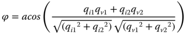
A recognized feature of forward faults is that they cause superimposed voltages and currents with different sign [3]. Thus, the rule to determine the fault direction is: ϕ close to 180° denotes fault in the forward direction and ϕ close to 0° denotes a reverse (backward) fault (see Figure 17.3). Hence, a forward fault has to fulfill:
Where δ gives a confidence interval for the possible variations of ϕ, and must be set in accordance to precomputed training faults.
Figure 17.2 Directional protection, general scheme.
Figure 17.3 Representation of voltage and current signals in the EOF plane for: (a) forward fault and (b) backward fault.
17.3.2 Fault Classification
In order to minimize the impact on power quality and continuity after a contingency, it is required to disconnect as few devices as possible from the power network. Single phase to ground faults have a higher probability of occurrence than multiphase faults. Thus, single pole tripping (SPT) schemes are implemented for improving selectivity in transmission system protection. SPT enhances the stability, power transfer capabilities, reliability, and availability of a transmission system during and after a single phase to ground fault [21, 22]. Furthermore, accurate SPT accompanied with automatic reclosing allows greater improvement of power system stability [23]. Therefore, in order to enable SPT and auto reclosing schemes, a method for classifying faults is essential.
17.3.2.1 Required EOF
For fault direction, data analysis of fault data is focused only on the first two EOFs, which normally contain more than 90% of data variability. However, information provided by f1(t) and f2(t) is not sufficient for fault classification, since faults of different types can have similar values in this space. Hence, in order to achieve an effective fault classification, those EOFs with smaller variances should be also considered, since they provide significant information of fault characteristics.
17.3.2.2 Fault Type Surfaces
A training database in the EOF space X(q) contains the coefficients of training faults decomposed in terms of the r selected EOFs. X(q) includes observations of the six possible fault types (ABC, AB, ABG, AC, ACG, and AG), which describes a perfectly defined r-dimension pattern, where fault location and fault inception angle patterns are relevant.
During the fault simulation stage, only a representative sample of possible faults is generated for training data. With the purpose of covering the entire fault type surface, formed in the r-dimensional space given by the selected EOF, the reference data is enlarged with estimated observations created by interpolation in accordance with the fault location and inception angle patterns.
17.3.2.3 Defining the Fault Type
Figure 17.4 presents the scheme for fault classification. After an event is detected, the relay extracts the superimposed current quantity sampled with the same data window and sampling frequency of the EOF. The discrete signal obtained is decomposed with the selected EOF, and the resultant vector is:
The fault type is identified using k-nearest neighbor classification (kNN). Here, the evaluated signal ![]() is assigned to the class of its nearest (most similar) sample in the database Y(q). Different metrics can be used to find the k-nearest neighbor points, for instance: city block, Euclidean, or cosine distance. Cosine distance (17.19) is recommended since it evaluates the angle between the two vectors, and it is independent from vectors magnitude. This metric improves classification for ground contact faults, because fault resistance influences the current magnitude but not its angle.
is assigned to the class of its nearest (most similar) sample in the database Y(q). Different metrics can be used to find the k-nearest neighbor points, for instance: city block, Euclidean, or cosine distance. Cosine distance (17.19) is recommended since it evaluates the angle between the two vectors, and it is independent from vectors magnitude. This metric improves classification for ground contact faults, because fault resistance influences the current magnitude but not its angle.

where ![]() is a reference fault current that belongs to the reference database Y(q), and r is the number of selected EOFs. Additionally, when the evaluated event is a fault occurring in the protected transmission line, the minimum distance between
is a reference fault current that belongs to the reference database Y(q), and r is the number of selected EOFs. Additionally, when the evaluated event is a fault occurring in the protected transmission line, the minimum distance between ![]() and Y(q) is small; then, a maximum distance dref can be established as a first criterion to classify the event as an internal fault (inside the protected transmission line), non-fault event, or external fault.
and Y(q) is small; then, a maximum distance dref can be established as a first criterion to classify the event as an internal fault (inside the protected transmission line), non-fault event, or external fault.

Figure 17.4 Fault classification and fault location, general scheme.
In order to improve the security of this classification method, an additional criterion is included for choosing the more severe fault type in the case that the k-nearest neighbor classification faces a conflict—for instance, two surfaces with similar nearest neighbors to the evaluated fault.
17.3.3 Fault Location
This function uses information from the classification function (see Figure 17.4). After the fault type is defined, the evaluated fault is assumed to have the same features as the nearest reference fault. This methodology obtains the reference fault that is most similar to the evaluated fault. This reference fault has inception angle and fault location previously defined and, if the distance metric is relatively small, the analyzed fault could directly be matched to the closer reference fault.
17.4 Study Case
17.4.1 Transmission Line Model and Simulation
Modeling the line to be protected and their neighbor lines is the first step to be carried out in order to get a fault database that describe the fault behavior of the transmission line, which will be then used for obtaining the EOF that describe the faults affecting the analyzed line and is required as reference for setting the protection functions.
Adequate models and software have to be used in order to get a precise emulation of the real transmission line. This part can be given as a limitation of the present approach, because of the difficulty of definition of an adequate model and software. Nevertheless, electromagnetic transient programs based on the EMTP method, proposed by Dommel in 1969 [24] and enhanced over the years with additional contributions [6], have demonstrated accuracy and reliability by a number of test cases [25]. Additionally, the representation of the frequency dependent parameters of a transmission line [26] denotes efficiency and accuracy for most simulation cases.
Because of the deterministic nature of the protection algorithm to be proposed, an important number of faults have to be generated for different conditions of location, fault inception angle (θ0), fault resistance (Rf), and fault type, so that the algorithm will consider a representative sample of the possible faults that could appear in the studied transmission lines. Table 17.1 summarizes typical conditions employed for fault simulation.
Table 17.1 Conditions for fault simulation
| Feature | Range | Detail |
| Fault Type | 1φg, 2φ, 2φg, 3φ | All fault types affecting the line |
| Inception Angle θ0 (deg) | 0, 30,…, 330 | From 0° to 360°, with 30° step |
| Fault Location (km) | 1, 10, 20, … L | From 0 to line length, with 10 km step |
| Fault Resistance Rf (Ω) | 0, 5, 40, 100 | Or in accordance with typical values |
Simulating a great number of faults is actually not difficult; a MATLAB application is developed in order to command the required simulations in the created EMTP model [27].
17.4.2 The Power System and Transmission Line
The Western System Coordinating Council (WSCC) 3-Machine 9-Bus test system [28] (see Figure.17.5) is evaluated in ATP/EMTP. The longest transmission line (line B6-B9, 180 km) is studied. Line B6-B9 and its adjacent lines B4-B6 (96 km) and B8-B9 (108 km) are modeled using the frequency dependent model of J. Martí [26], which provides an accurate and reliable time domain model for electromagnetic transients simulations. See model data in Appendix A. Fault signals are registered in relay R6 located at bus B6.
Figure 17.5 Nine-bus test system implemented in ATP.
17.4.3 Training Data
With the intention of establishing the accurate pattern exhibited by fault waveforms, a vast number of faults are computer-generated for different conditions of type, fault inception angle (θ0), fault resistance (Rf), and location. The sampling technique aims to get enough information on the faults that could appear along the line; then the data obtained should serve as a good representation of the total population. The fault conditions used are detailed in Table 17.2 and Table 17.3.
Table 17.2 Forward faults (line B6-B9)
| FaultType | Inception Angle (deg) | Rf (Ω) | Fault Locationfrom B6 (km) |
| ABC | 0, 30,…, 330 | − | 1, 10, 20, …180 |
| ABG | 0, 30,…, 330 | 5 | 1, 10, 20, …180 |
| AB | 0, 30,…, 330 | − | 1, 10, 20, …180 |
| ACG | 0, 30,…, 330 | 5 | 1, 10, 20, …180 |
| AC | 0, 30,…, 330 | − | 1, 10, 20, …180 |
| AG | 0, 30,…, 330 | 40 | 1, 10, 20, …180 |
Table 17.3 Reverse faults (line B4-B6)
| FaultType | Inception Angle (deg) | Rf (Ω) | Fault Locationfrom B6 (km) |
| ABC | 0, 30,…, 330 | − | 1, 10, 20, …90 |
| ABG | 0, 30,…, 330 | 5 | 1, 10, 20, …90 |
| AB | 0, 30,…, 330 | − | 1, 10, 20, …90 |
| ACG | 0, 30,…, 330 | 5 | 1, 10, 20, …90 |
| AC | 0, 30,…, 330 | − | 1, 10, 20, …90 |
| AG | 0, 30,…, 330 | 40 | 1, 10, 20, …90 |
17.4.4 Training Data Matrix
The training data matrix is composed by faults described in Table 17.2. From a data mining perspective, every discrete current or voltage fault signal xi(t) is an observation, and the samples of each signal are their features. This set of signals is represented by the n×p data matrix X shown in (17.1).
17.4.4.1 Data Window
Defining the time window length is a crucial aspect in the design of a protection algorithm. The longer the time window, the more information it provides, whereas a shorter time window yields high-speed decision making. In the present analysis, time windows in the order of 600 µs are used, which is long enough to observe the evident patterns of fault generated transients and avoids reflected waves from the remote bus affecting the wave shape of signals measured by relay R6 (see Figure. 17.6). A methodology such as that proposed in [29] can be used to detect the initial wavefront.
Figure 17.6 Effect of reflected waves from remote node (Node B4), for the following configurations: one power transformer and (i) two transmission lines, (ii) three transmission lines, (iii) four transmission lines. For twice the traveling time of the neighbor line (640 µs), there is no significant change in the signal waveform.
17.4.4.2 Sampling Frequency
In a transmission line, frequencies in the order of some hundreds of kHz are expected in fault generated transients. By virtue of Nyquist's theorem, the sampling frequency should be twice that frequency if the entire frequency spectrum is taken into account, which means an additional cost in the sampling process during A/D conversion. However, the sampling frequency should be distinguished depending on the protection function to be implemented, for instance a directional function is associated with the two firsts EOFs only, which are related to low frequency patterns and therefore they are scarcely affected by high frequency components [14, 16]. Hence, not too high a sampling frequency is required for pattern based directional protection. On the other hand, fault classification and location can require the identification of high frequency patterns, thus a high sampling frequency is necessary in this function. In the following sections, various sampling frequencies are studied in order to show the effect of this variable on the signal patterns.
17.4.5 Signal Conditioning
17.4.5.1 Superimposed Component
The pre-fault component is removed from fault signals, by means of (17.20), in order to obtain the superimposed component introduced by the fault:
where:
 is the generated deviations from the steady-state signals;
- x(t)is the discrete signal obtained from the model;
- xS(t) is the pre-fault signal.
A common practice to derive the incremental magnitudes is using the signals measured exactly one cycle before the actual measurement. This can be achieved, for instance, by using a delta filter [30]. Another practice is using high-pass filters to suppress the steady-state components so that only the high frequency components will be present in the relaying signals [3].
The data matrix of fault signals (voltages or currents) is formed with the superimposed components ![]() :
:
17.4.5.2 Centering the Variables
An essential condition for applying EOFs is removing the mean of each variable from the data set in order to center the data on the origin. This process does not change the EOFs, because they are obtained from the variance–covariance matrix, which is computed from the centered data. However, for a new signal that is going to be compared with predefined faults, it must be centered using the mean vector of the training data matrix.
17.4.5.3 Scaling
In some cases, such as for implementing the pattern based directional function, data can be scaled to set data in a common scale independent from measurement units. In this case, the coefficients of the training matrix are scaled between -1 and 1 by dividing by the maximum absolute coefficient; this last operation does not affect the data shape.
For protection functions such as fault classification and location, data scaling is not recommended since the fault magnitude contributes to adequate fault classification.
17.4.6 Energy Patterns
An alternative for categorizing a transient event is by evaluating the energy associated to voltage and current waveforms. In signal processing, the energy Ei of a p-length discrete signal ![]() is computed by:
is computed by:

Where ![]() is the time interval between each sample of the discrete signal. The mean power Pi and the RMS value in the interval
is the time interval between each sample of the discrete signal. The mean power Pi and the RMS value in the interval ![]() are given by:
are given by:


The RMS value as a measure of energy was evaluated for the group of fault current signals generated with the conditions detailed in Table 17.2. Results highlight that faults of the same type follow a defined pattern governed by a fault inception angle pattern and a fault location pattern (see Figures 17.7 and 17.8).
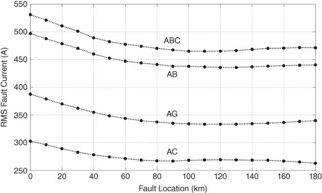
Figure 17.7 RMS fault current, fault type, and fault location pattern,  , data window = 600 µs.
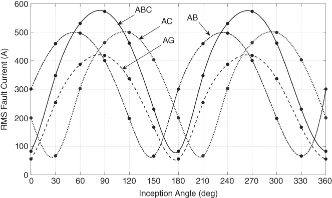
Figure 17.8 RMS fault current, fault type, and fault inception angle pattern, location = 1 km, data window = 600 µs.
Combination of both characteristics (location and inception angle) for single phase to ground faults (AG) with ![]() is presented in Figure 17.9. Here is can be seen that faults of the same type, in this case single phase to ground faults, have a defined place in the demarked surface.
is presented in Figure 17.9. Here is can be seen that faults of the same type, in this case single phase to ground faults, have a defined place in the demarked surface.
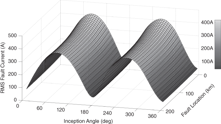
Figure 17.9 RMS fault current, fault inception angle and location pattern for AG faults,  .
.
The data window plays an important role in the patterns defined by the RMS values of fault currents. Longer data windows have more information and hence allow major differentiation between fault signals. For example, see in Figure 17.10 how the location of a fault can be distinguished using longer data windows. Nonetheless, longer signals (in terms of time) contain transient components altered at remote nodes, and therefore they are affected by the configuration of those nodes (see Figure 17.11). Although this aspect is not a major limitation, it has to be considered in the design of the protection algorithm.
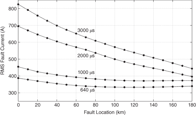
Figure 17.10 RMS fault current, fault location pattern for different data windows, θ0 = 90°.
Figure 17.11 RMS fault current, fault location pattern for different θ0, data window = 3 ms.
In general, the energy associated with faulted signals is higher than the energy of non-fault signals. However, some faults can generate signals with relatively low associated energy: such is the case of high impedance faults (HIF) or faults that could occur with small inception voltage. On the other hand, some non-fault transients can produce signals with high energy: for instance, transmission line or capacitor bank switching. A mechanism to distinguish faults arising on the protected device and external faults is also necessary since both can produce high energy signals. Here, EOF decomposition plays an important role because EOFs can be used to decompose energy patterns into an n-dimension space that retains the dominant patterns of data processed.
17.4.7 EOF Analysis
17.4.7.1 Computing the EOFs
The training data matrix is composed of the faults detailed in Table 17.2. That is, the data matrix contains 6 fault types, 12 fault inception angles, and 19 fault locations. That gives a total of 1368 (6×12×19) faults. Each current signal is a 600 µs discrete-time series. The number of samples in each signal will depend on the sampling frequency. Different sampling frequencies ( fs) are studied in order to show the incidence of this variable in the EOF. The left singular vectors and their related eigenvalues of the data matrix are computed. Explained variability EV of the first eight EOF is summarized in Table 17.4.
Table 17.4 Explained variability of the first eight EOFs for different sampling frequencies, data window 600 µs
| fs | EV(%)a | ||||||||
| EOF1 | EOF2 | EOF3 | EOF4 | EOF5 | EOF6 | EOF7 | EOF8 | ||
| 1 MHz | 1 µs | 79.08 | 12.90 | 3.96 | 2.28 | 0.53 | 0.45 | 0.22 | 0.14 |
| 200 kHz | 5 µs | 79.70 | 12.50 | 4.04 | 2.17 | 0.62 | 0.38 | 0.19 | 0.11 |
| 100 kHz | 10 µs | 82.80 | 11.25 | 3.63 | 1.58 | 0.31 | 0.15 | 0.09 | 0.05 |
| 50 kHz | 20 µs | 88.86 | 8.84 | 1.71 | 0.26 | 0.12 | 0.06 | 0.04 | 0.02 |
| 20 kHz | 50 µs | 94.37 | 4.83 | 0.58 | 0.10 | 0.05 | 0.03 | 0.01 | 0.01 |
a Variability percentage from original data retained by each EOF.
From the results presented in Table 17.4, we can draw out some important features of the EOFs:
- a. The two first EOFs (EOF1 and EOF2) represent the dominant pattern since they attain more than 90% of EV in all the cases. This is in fact one of the advantages of EOF decomposition: that most of the variation presented in the original signals is retained in the first EOF.
- b. The EV of EOF1 is greater for lower sampling frequencies. This means that the main EOF (EOF1) is associated with a low frequency pattern.
From the last remark, we can state a relationship between the EOF order and the frequency. From experiences with different transmission lines it has been observed that the first EOF associated with larger eigenvalues is related to low frequencies patterns. That is, the higher the order of the EOF, the higher its frequency (see Figure 17.12). This statement is also mentioned in [14] where Hannachi et al. maintain that “high/low power are associated respectively with low/high frequency variability. Hence low frequency and large scale patterns tend to capture most of the variance observed in the system.” The aforementioned property makes the first EOFs (principal components) immune to noise as is also stated in [16].

Figure 17.12 Coefficients of the first twelve EOFs, 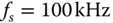 .
.
Figure 17.13 shows the waveform of EOF1 and EOF2 for different sampling frequencies. As can be seen, they are barely affected by the sampling frequency. This occurs because these EOFs represent low frequency patterns and therefore they are not altered by the high frequencies of fault generated transients.

Figure 17.13 Effect of sampling frequency in the two first EOFs.
17.4.7.2 Fault Patterns Using EOF
Consider ![]() . For this sampling frequency, it can be observed in Table 17.4 that the first three EOFs have more than 99% of the overall explained variability. That is, the entire group of analyzed faults can be decomposed in terms of only three EOFs with less than 1% loss of information:
. For this sampling frequency, it can be observed in Table 17.4 that the first three EOFs have more than 99% of the overall explained variability. That is, the entire group of analyzed faults can be decomposed in terms of only three EOFs with less than 1% loss of information:
Expression (17.8) shows that coefficients qij are computed by correlating the ith signal with the associated jth EOF. The coefficients qij also presents fault location and fault inception angle patterns similar to energy patterns (see Figures 17.17 and 17.18), presented in Section 14.5. However, the orthogonal decomposition allows representing these patterns in an optimal multidimensional space. For instance, in Figure 17.14, faults generated along the line with the same fault inception angle ![]() are projected into a 2-dimensional space conformed by the first two EOF. In this projection, different fault types are well-differentiated.
are projected into a 2-dimensional space conformed by the first two EOF. In this projection, different fault types are well-differentiated.
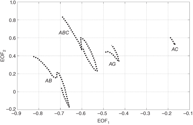
Figure 17.14 Different fault types in the two first EOF, fault location from 0 to 180 km,  .
.
Results show that even though the fact that faults may appear under (theoretically) infinite stochastic conditions (i.e., fault location, inception angle, fault resistance, and number of involved phases), the waveforms of faulted signals follow a well-defined deterministic behavior. Therefore, it is not necessary to consider the infinite possible fault conditions in order to attain generalized EOFs. In fact, just a small representative sample of different fault conditions is required to achieve a good representation of the total population.
17.4.8 Evaluation of the Protection Scheme
17.4.8.1 Fault Direction
Phase A to ground (AG) fault currents projected in the EOF plane are presented in Figure 17.15. Here, twelve clusters, corresponding to the twelve θ0 used in the training data, are defined. Each point in Figure 17.15a represents a fault with specific θ0 and fault location. The corresponding forward fault voltages are presented in Figure 17.15b: it can be observed that forward voltage signals in the EOF plane appear around 180° away from the respective current signal.
Figure 17.15 Forward single phase to ground faults (AG),  , representation on the first two EOFs, (a) current signals, (b) voltage signals.
On the other hand, backward faults cause voltages and currents with similar angle in the EOF plane denoted by f1(t) and f2(t). Figure 17.16 presents the current and voltage signals generated by backward single phase to ground faults (AG).
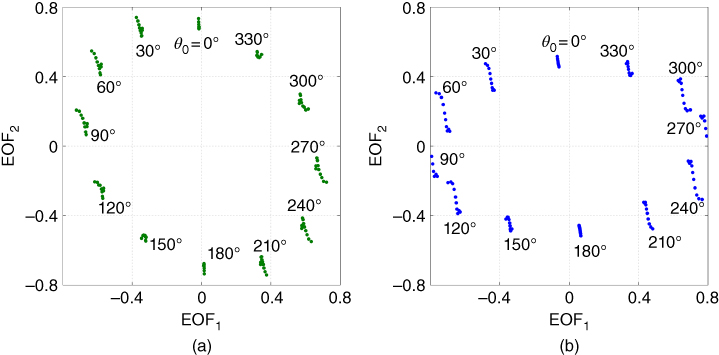
Figure 17.16 Backward single phase to ground faults (AG),  , representation on the first two EOFs, (a) current signals, (b) voltage signals.
17.4.9 Fault Classification
In order to obtain reference surfaces for fault classification, a cubic spline data interpolation is employed. Fault location patterns are interpolated from 0 to 180 km with a 2 km step; Angle patterns are interpolated from 0 to 355° with 5° step. Examples of fault location and inception angle interpolation are presented in Figures 17.17 and 17.18. After interpolation, original data grows from 1368 observations to a database with 39 312 observations per fault type, which are stored in matrix Y(q). Figure 17.19 shows the three-dimensional surface of ABG and AG faults for inception angles from 0° to 355°, plotted with interpolated data.
Figure 17.17 Interpolation of fault location pattern for AG faults,  .
.
Figure 17.18 Interpolation of inception angle pattern for ABG faults,  .
.
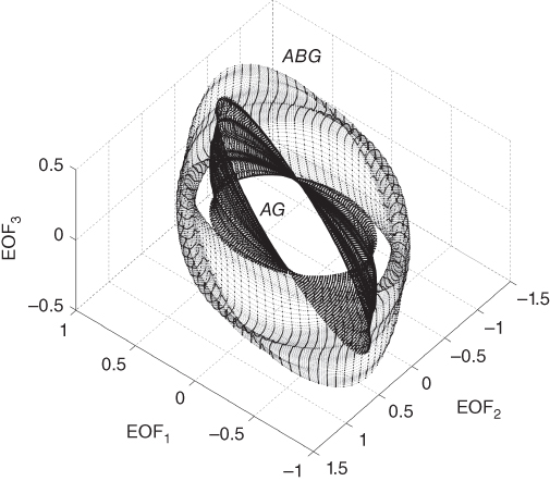
Figure 17.19 Three-dimensional representation of ABG and AG current faults using the three first EOFs. Fault location from 0 to 180 km, fault inception from 0 ° to 355 °.
17.4.9.1 Classification
The faults detailed in Table 17.5 were evaluated with the proposed classification scheme. At first, the training stage considered different classification parameters in order to find the best kNN classifier. For the present case study, the optimal classification parameters are as follows. Sampling frequency: 200 kHz; selected EOF: from 1 to 12; distance metric: cosine; number of nearest neighbors: 1. Results are presented in Table 17.6: it can be seen that accuracy for AG faults is 100%, which means that no multiphase fault was classified as a single phase to ground fault AG, which is important for security. Nevertheless, accuracy for multiphase faults is reduced; most confusion appears between faults that involve the same phases, that is, AB with ABG or AC with ACG. Almost all the AG faults that where classified as two phase faults correspond to faults with fault resistance ![]() . Recall that the reference database only considered AG for
. Recall that the reference database only considered AG for ![]() . Hence, classification accuracy could be improved by incorporating one or two more AG surfaces for different fault resistances.
. Hence, classification accuracy could be improved by incorporating one or two more AG surfaces for different fault resistances.
Table 17.5 Test faults, line B6-B9
| FaultType | Inception Angle (deg) | Rf(Ω) | Fault Locationfrom B6 (km) |
| ABC | 0, 30,…, 330 | – | 5, 15, 25, …175 |
| ABG | 0, 30,…, 330 | 5 15 |
5, 15, 25, …175 1, 5, 10, …180 |
| AB | 0, 30,…, 330 | – | 5, 15, 25, …175 |
| ACG | 0, 30,…, 330 | 5 15 |
5, 15, 25, …175 1, 5, 10, …180 |
| AC | 0, 30,…, 330 | – | 5, 15, 25, …175 |
| AG | 0, 30,…, 330 | 40 0, 20, 100, 300 |
5, 15, 25, …175 1, 5, 10, …180 |
Table 17.6 Classification results, confusion matrix
| ABC | ABG | AB | ACG | AC | AG | Accuracy | |
| ABC | 213 | 0 | 0 | 4 | 0 | 0 | 98.16% |
| ABG | 0 | 632 | 8 | 0 | 0 | 4 | 98.14% |
| AB | 2 | 28 | 208 | 2 | 0 | 3 | 85.60% |
| ACG | 1 | 0 | 0 | 638 | 6 | 16 | 96.52% |
| AC | 0 | 0 | 0 | 16 | 210 | 26 | 83.33% |
| AG | 0 | 0 | 0 | 0 | 0 | 1943 | 100.00% |
| Sensitivity | 98.61% | 95.76% | 96.30% | 96.67% | 97.22% | 97.54% | 97.07% |
17.4.10 Fault Location
Results of fault location are summarized in Table 17.7. For the 3960 test faults of Table 17.5, 2630 (66.41%) were located with 100% accuracy (0 km error), and only 131 faults (3.31%) present inaccuracy greater than 5 km. Most inaccuracies greater than 5 km are found in single phase to ground faults with ![]() and
and ![]() . Some examples of fault location are shown in Table 17.8: it can be seen that greater inaccuracies appear for AG faults
. Some examples of fault location are shown in Table 17.8: it can be seen that greater inaccuracies appear for AG faults ![]() . As aforementioned, accuracy of fault location can be improved by incorporating more AG surfaces for different fault resistances.
. As aforementioned, accuracy of fault location can be improved by incorporating more AG surfaces for different fault resistances.
Table 17.7 Results of fault location
| Error (km) | Number of Faults | % |
| 0 | 2630 | 66.41 |
| 1 | 751 | 18.96 |
| 2 | 202 | 5.10 |
| 3 | 123 | 3.11 |
| 4 | 95 | 2.40 |
| 5 | 28 | 0.71 |
| >5 | 131 | 3.31 |
Table 17.8 Some results of fault classification
| Evaluated Fault | Nearest Reference Fault | Location Error (km) | ||||||
| Fault Type | θ0 | Rf (Ω) | L (km) | Fault Type | θ0 | Rf(Ω) | L (km) | |
| ABC | 90° | – | 15 | ABC | 90° | – | 13 | 2 |
| ABG | 90° | 5 | 25 | ABG | 85° | 5 | 25 | 0 |
| ABG | 60° | 15 | 65 | ABG | 55° | 5 | 66 | 1 |
| AB | 30° | – | 95 | ABG | 50° | 5 | 93 | 2 |
| ACG | 0° | 15 | 165 | ACG | 355° | 5 | 166 | 1 |
| AC | 60° | – | 115 | AC | 60° | – | 115 | 0 |
| AG | 60° | 20 | 135 | AG | 55° | 40 | 133 | 2 |
| AG | 120° | 0 | 85 | AG | 120° | 40 | 88 | 3 |
| AG | 150° | 100 | 170 | AG | 155° | 40 | 171 | 1 |
| AG | 60° | 300 | 95 | AG | 55° | 40 | 96 | 1 |
| AG | 90° | 300 | 135 | AG | 125° | 40 | 156 | 21 |
| AG | 30° | 300 | 125 | ACG | 50° | 5 | 142 | 17 |
| AG | 150° | 300 | 115 | AG | 145° | 40 | 102 | 13 |
17.5 Conclusions
Empirical orthogonal functions appear to be a promising alternative for signal processing applied to fault diagnosis. Results show that in spite of the fact that faults may appear under infinite stochastic conditions such as fault location, inception angle, fault resistance, pre-fault current, and number of involved phases, the waveforms of faulted signals follow a well-defined deterministic pattern. The proposed methodology can obtain precise information on a fault by evaluating a very short signal (600 µs for the presented case study), which is really valuable for implementation in high-speed protection schemes.
The proposed protection scheme uses kNN for fault classification and location, which is a very simple classification method. In fact, we highlighted that classification performance can be improved. Readers are encouraged to evaluate more sophisticated classification methods such as support vector machines and other kernel based classifiers.

Figure 17.20 WECC 9-bus test system, ATPDraw Model.
Appendix 17.A
Study Cases: WECC 9-bus, ATPDraw Models and Parameters
Figure 17.20 shows the WECC 9-bus power system. Lines B4-B5, B5-B7, and B7-B8 are implemented with the 3-phase distribution parameter transposed line Clarke model; transmission lines B4-B6, B6-B9, and B8-B9 are modeled in a more detailed fashion. These lines have three transposition points and eight line segments for simulating faults along the line—see Figure 17.21. Every line segment uses the JMarti model with the data presented in Table 17A.1. Particular data for each line are presented in Tables 17A.2, 17A.3 and 17A.4.
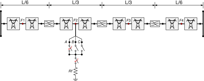
Figure 17.21 Detailed transmission line model including a fault circuit.
Table 17A.1 ATPdraw line/cable model, lines: B4-B6, B6-B9, and B8-B9
| Model: | JMarti | Ground resistivity (Ωm): | 100 |
| Type: | Overhead line | Initial freq. (Hz): | 0.1 |
| Number of phases: | 3 | Decades: | 7 |
| Transposed: | Inactive | Points/dec: | 100 |
| Auto bundling: | Inactive | Freq. matrix (Hz): | 3000 |
| Skin Effect: | Active | Freq. SS (Hz): | 60 |
| Segmented ground | Inactive | Use default fitting | Active |
| Real transf. matrix | Inactive |
Table 17A.2 ATPdraw line/cable data, line B4-B6
| # | Ph.No. | Rin(cm) | Rout(cm) | DC Res. (Ω/km) | Horiz(m) | Vtower(m) | Vmin(m) |
| 1 | 1 | 0.4134 | 1.2408 | 0.0918 | −6.5 | 18 | 7.1 |
| 2 | 2 | 0.4134 | 1.2408 | 0.0918 | 0 | 18 | 7.1 |
| 3 | 3 | 0.4134 | 1.2408 | 0.0918 | 6.5 | 18 | 7.1 |
| 4 | 0 | 0.4626 | 0.771 | 0.3002 | −4 | 22.35 | 14.5 |
| 5 | 0 | 0.4626 | 0.771 | 0.3002 | 4 | 22.35 | 14.5 |
Table 17A.3 ATPdraw line/cable data, line B6-B9
| # | Ph.No. | Rin(cm) | Rout(cm) | DC Res.(Ω/km) | Horiz(m) | Vtower(m) | Vmin(m) |
| 1 | 1 | 0.492 | 1.148 | 0.1141 | −6.5 | 18 | 8.6 |
| 2 | 2 | 0.492 | 1.148 | 0.1141 | 0 | 18 | 8.6 |
| 3 | 3 | 0.492 | 1.148 | 0.1141 | 6.5 | 18 | 8.6 |
| 4 | 0 | 0.4626 | 0.771 | 0.3002 | −4 | 22.35 | 14.5 |
| 5 | 0 | 0.4626 | 0.771 | 0.3002 | 4 | 22.35 | 14.5 |
Table 17A.4 ATPdraw line/cable data, line B8-B9
| # | Ph.No. | Rin(cm) | Rout(cm) | DC Res.(Ω/km) | Horiz(m) | Vtower(m) | Vmin(m) |
| 1 | 1 | 0.527 | 1.581 | 0.0561 | −6.5 | 18 | 7.1 |
| 2 | 2 | 0.527 | 1.581 | 0.0561 | 0 | 18 | 7.1 |
| 3 | 3 | 0.527 | 1.581 | 0.0561 | 6.5 | 18 | 7.1 |
| 4 | 0 | 0.4626 | 0.771 | 0.3002 | −4 | 22.35 | 14.5 |
| 5 | 0 | 0.4626 | 0.771 | 0.3002 | 4 | 22.35 | 14.5 |
The resultant impedances and admittances for lines B4-B6, B6-B9, and B8-B9 are presented in Table 17A.5.
Table 17A.5 Line impedances and admittances
| Line | Sequence | Impedance(ohm/km) | Admittance(mho/km) | Surge Impedance(ohm) | Surge Velocity(km/s) |
| B4 – B6 | 0 | 0.2643+j0.9821 | j2.4178×10−6 | 648.5–j7.5 | 2.425×10⁵ |
| 1 | 0.0934+j0.5033 | j3.2944×10−6 | 394.2–j5.3 | 2.915×10⁵ | |
| B6 – B9 | 0 | 0.2891+j0.9685 | j2.3901×10−6 | 650.2–j8.3 | 2.451×10⁵ |
| 1 | 0.1157+j0.5069 | j3.2539×10−6 | 399.7–j6.4 | 2.917×10⁵ | |
| B8 – B9 | 0 | 0.2281+j0.9699 | j2.4917×10−6 | 632.4–j6.6 | 2.408×10⁵ |
| 1 | 0.0581+j0.4850 | j3.4260×10−6 | 377.6–j3.4 | 2.919×10⁵ |
References
- 1 Q. H. Wu, Z. Lu, and T. Ji, Protective Relaying of Power Systems Using Mathematical Morphology, 1st ed. Liverpool: Springer, 2009.
- 2 M. S. Sachdev et al., “Understanding Microprocessor-Based Technology Applied to Relaying,” Power System Relaying Committee, Atlanta, 2009.
- 3 A. T. Johns and S. K. Salman, Digital Protection for Power Systems, 1st ed. London: Peter Peregrinus, 1997.
- 4 Z. Q. Bo, F. Jiang, Z. Chen, X. Z. Dong, G. Weller, and M. A. Redfern, “Transient Based Protection for Power Transmission Systems,” in IEEE PES Winter Meeting, Singapore, 2000, vol. 3, pp. 1832–1837.
- 5 Z. Q. Bo, G. Weller, F. T. Dai, and Q. X. Yang, “Transient Based Protection for Transmission Lines,” in Proceedings of International Conference on Power System Technology (POWERCON), 1998, vol. 2, pp. 1067–1071.
- 6 N. Watson and J. Arrillaga, Power Systems Electromagnetic Transients Simulation, 1st ed. London: Institution of Engineering and Technology, 2002.
- 7 A. R. Messina and V. Vittal, “Extraction of Dynamic Patterns From Wide-Area Measurements Using Empirical Orthogonal Functions,” IEEE Trans. Power Syst., vol. 22, no. 2, pp. 682–692, May 2007.
- 8 P. Esquivel and A. R. Messina, “Complex Empirical Orthogonal Function analysis of wide-area system dynamics,” in 2008 IEEE Power and Energy Society General Meeting - Conversion and Delivery of Electrical Energy in the 21st Century, 2008, pp. 1–7.
- 9 R. P. Aguilar, F. E. Perez, E. A. Orduna, and N. J. Castrillon, “Empirical orthogonal decomposition applied to transmission line protection,” in 2011 IEEE PES Conference on Innovative Smart Grid Technologies (ISGT Latin America), 2011, pp. 1–7.
- 10 R. Aguilar, F. Perez, E. Orduna, and C. Rehtanz, “The Directional Feature of Current Transients, Application in High-Speed Transmission-Line Protection,” IEEE Trans. Power Deliv., vol. 28, no. 2, pp. 1175–1182, 2013.
- 11 J. C. Cepeda and D. G. Colomé, “Benefits of empirical orthogonal functions in pattern recognition applied to vulnerability assessment,” in Transmission Distribution Conference and Exposition - Latin America (PES T D-LA), 2014 IEEE PES, 2014, pp. 1–6.
- 12 E. N. Lorenz, “Empirical Orthogonal Functions and Statistical Weather Prediction,” Dept. of Meteorology, MIT, Massachusetts, Scientific Report 1, 1956.
- 13 I. T. Jolliffe, Principal Component Analysis, 2nd ed. New York: Springer-Verlag, 2002.
- 14 A. Hannachi, I. T. Jolliffe, and D. B. Stephenson, “Empirical Orthogonal Functions and Related Techniques in Atmospheric Science: a Review,” Int. J. Climatol., vol. 27, no. 9, pp. 1119–1152, Jul. 2007.
- 15 E. Vazquez, I. I. Mijares, O. L. Chacon, and A. Conde, “Transformer Differential Protection Using Principal Component Analysis,” IEEE Trans. Power Deliv., vol. 23, no. 1, pp. 67–72, Jan. 2008.
- 16 P. Jafarian and M. Sanaye-Pasand, “A Traveling-Wave-Based Protection Technique Using Wavelet/PCA Analysis,” IEEE Trans. Power Deliv., vol. 25, no. 2, pp. 588–599, Apr. 2010.
- 17 R. Aguilar, F. Pérez, and E. Orduña, “High-Speed Transmission Line Protection Using Principal Component Analysis, a Deterministic Algorithm,” IET Gener. Transm. Distrib., vol. 5, no. 7, pp. 712–719, Jul. 2011.
- 18 J. A. Morales and E. Orduna, “Patterns Extraction for Lightning Transmission Lines Protection Based on Principal Component Analysis,” IEEE Lat. Am. Trans., vol. 11, no. 1, pp. 518–524, Feb. 2013.
- 19 Y. Wang, J. Zhou, Z. Li, Z. Dong, and Y. Xu, “Discriminant-Analysis-Based Single-Phase Earth Fault Protection Using Improved PCA in Distribution Systems,” IEEE Trans. Power Deliv., vol. 30, no. 4, pp. 1974–1982, Aug. 2015.
- 20 D. Randall, “Empirical Orthogonal Functions,” Department of Atmospheric Science, Colorado State University, Colorado, USA, Jan. 2003.
- 21 F. Calero and D. Hou, “Practical considerations for single-pole-trip line-protection schemes,” in 58th Annual Conference for Protective Relay Engineers, 2005., 2005, pp. 69–85.
- 22 D. W. P. Thomas, M. S. Jones, and C. Christopoulos, “Phase Selection Based on Superimposed Components,” Transm. Distrib. IEE Proc. - Gener., vol. 143, no. 3, pp. 295–299, May 1996.
- 23 W. M. Al-hassawi, N. H. Abbasi, and M. M. Mansour, “A neural-network-based approach for fault classification and faulted phase selection,” in Canadian Conference on Electrical and Computer Engineering, 1996, 1996, vol. 1, pp. 384–387 vol. 1.
- 24 H. W. Dommel, “Digital Computer Solution of Electromagnetic Transients in Single-and Multiphase Networks,” IEEE Trans. Power Appar. Syst., vol. PAS-88, no. 4, pp. 388–399, Apr. 1969.
- 25 A. Ametani, N. Nagaoka, Y. Baba, and T. Ohno, Power System Transients: Theory and Applications. CRC Press, 2013.
- 26 J. R. Marti, “Accuarte Modelling of Frequency-Dependent Transmission Lines in Electromagnetic Transient Simulations,” IEEE Trans Power App Syst, vol. PAS-101, no. 1, pp. 147–157, Jan. 1982.
- 27 G. D. Guidi and F. E. Perez, “MATLAB program for systematic simulation over a transmission line in alternative transients,” presented at the International Conference on Power Systems Transients, Vancouver, Canada, 2013.
- 28 P. M. Anderson and A. A. Fouad, Power System Control and Stability, 2nd ed. John Wiley & Sons, 2002.
- 29 R. Aguilar, F. Perez, and E. Orduna, “Ultra-sensitive disturbances detection on transmission lines using principal component analysis,” in 24th IEEE Canadian Conference on Electrical and Computer Engineering (CCECE), Ontario, Canada, 2011, pp. 93–98.
- 30 G. Benmouyal and J. Roberts, “Superimposed quantities: Their true nature and application in relays,” in 30th Annual Western Protective Relay Conference, Spokane, 2003.