Chapter 15
Enhancement of Transmission System Voltage Stability through Local Control of Distribution Networks
Dr. Gustavo Valverde1, Dr. Petros Aristidou2 and Prof. Thierry Van Cutsem3
1>School of Electrical Engineering, University of Costa Rica, Costa Rica
2School of Electronic and Electrical Engineering, University of Leeds, United Kingdom
3Dept. of Electrical Engineering and Computer Science, University of Liege, Belgium
15.1 Introduction
The most noticeable developments foreseen in power systems involve Distribution Networks (DNs). Future DNs are expected to host a large percentage of renewable energy sources [1], and small Dispersed Generation Units (DGUs) at distribution level are expected to supply a growing percentage of demand [2]. This proliferation of DGUs and the advances in infocommunications are key drivers of the transformations seen today in DNs.
The increased penetration of DGUs has given rise to new operational problems in DNs, such as over-voltages and thermal overloads at times of high DG production and low load. In response to these problems, several DN control schemes have been proposed to dispatch the DGUs and ensure secure network operation [3]. For instance, in [4], two coordinated voltage control algorithms are proposed. The first is based on simple control rules in which the Load Tap Changer (LTC) of the main transformer is used to control voltages. If this action is unable to restore all network voltages within limits, the resource with the highest effect on the most problematic bus is selected. The second algorithm is based on optimization—more precisely, a mixed integer nonlinear programming problem is used to minimize costs of network losses and generation curtailment, subject to voltage limits, active and reactive power limits of Distributed Energy Resources (DER), and branch power flow limits. The discrete control variables contain transformer tap position and switched capacitors while the continuous variables are the set points of real and reactive power or terminal voltages of DER.
The reactive power coordination scheme presented in [5] minimizes the number of transformer tap operations while satisfying voltage limits of the feeder, branch flow constraints, and transformer capacity constraints. The work in [6] presents a voltage control scheme to coordinate the operation of multiple regulating devices and DGUs in Medium Voltage (MV) distribution systems under variability of system topology and DGU availability.
In [7], the authors propose a Model Predictive Control (MPC) approach to regulate DN voltages using DGUs coordinated with the main transformer's LTC. Due to the closed-loop nature of MPC, the proposed control scheme can account for model inaccuracies and failure or delays of the control actions. The authors showed that anticipation of future LTC actions provide better and more efficient control decisions. This work was later extended in [8] to incorporate congestion management of DN lines. Moreover, a variant MPC formulation is presented in [9]. Here, the objective is to minimize the deviations of DGU active and reactive powers from reference values. DGU powers are restored to their desired schedule as soon as operating conditions allow doing so. Three modes of operation of the proposed controller are presented, involving dispatchable units as well as DGUs operated to track maximum power output, as detailed in Chapter 14.
These advanced control schemes rely on modern communication infrastructure and are currently at the heart of Smart Grid developments. They offer an attractive alternative to expensive network reinforcement, as long as stressed operating conditions prevail for a limited duration only. In addition to alleviating DN problems, they provide the possibility to actively support the transmission grid, if the legislative framework allows it and the controllers are designed to do so.
This chapter demonstrates how such advanced DN control schemes, and in particular Volt-Var Control (VVC), can affect long-term voltage stability of Transmission Networks (TNs). VVC refers to the process of managing voltage levels and reactive power throughout a distribution grid. It involves controlling devices that inject or consume reactive power to regulate the voltage profile, collaborating with existing equipment that directly control DN voltages.
In traditional DNs, the primary components for controlling voltage are LTCs, voltage regulators, and capacitor banks. The first two refer to variable ratio transformers connecting the DN to the TN or placed within the DN, and adjusted to raise or lower voltage as required. Capacitor banks are connected through mechanical breakers to the distribution grid, and when activated they inject reactive power for voltage boosting and/or power factor correction.
Modern VVCs, such as the ones referred to this chapter, rely on an advanced communication infrastructure to coordinate DGUs to inject/consume reactive power to mitigate dangerously low or high voltage conditions. These controllers usually incorporate the actions of traditional devices, such as LTCs or the activation of capacitor banks.
Beyond maintaining a stable voltage profile, VVCs have other potential benefits. For example, by acting on reactive power flows in the DN, they can alleviate thermal overloads [8], correct the power factor at the connection point with the TN [10], or minimize network losses. Moreover, using DGUs located close to the loads, VVCs offer additional flexibility to perform load voltage reduction. This well-known technique exploits the load sensitivity to voltage to decrease the active and reactive power demand [11–13]. Although not as effective as (under-voltage) load shedding [14], it may be applied as a first line of defense [15] or to reduce peak demands and energy consumption [16, 17].
Finally, if the VVCs are extended to allow the control of flexible loads, storage units, or the active power output of DGUs, then great flexibility is offered to manage the DN and support the TN in case of emergencies.
The remainder of this chapter is organized as follows. Section 15.2 provides a brief review of long-term voltage instability mechanisms and some conventional solutions used today. Then, Section 15.3 analyzes the impact that VVCs can have on long-term voltage stability of TNs as well as the mechanisms available to enhance stability. In Sections 15.4 and 15.5, a combined Transmission and Distribution (T&D) test-system is used to provide an example of this behavior and some long-term instability countermeasures. Finally, conclusions are drawn in Section 15.6.
15.2 Long-Term Voltage Stability
Long-term voltage instability results from the inability of the combined transmission and generation system to deliver the power requested by loads at least at some nodes [11, 18, 19]. It is a slow phenomenon with a timescale of up to several minutes. This type of instability usually occurs when the system is highly stressed (high demand of active and reactive power) and is initiated by component outages (line, transformer, generator, etc.). Some of the driving forces behind long-term voltage instability are the lack of fast reactive power resources, the action of OverExcitation Limiters (OELs) enforcing generator reactive power limits, and load power restoration. The last of these can be due to the LTCs trying to recover DN voltages, and therefore the load powers, or even due to the self-restoration of loads.
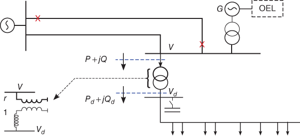
Figure 15.1 Simple T&D system with DN controlled by LTC.
Long-term voltage instability is caused by the non-existence of a post-disturbance equilibrium or the lack of attraction towards the stable post-disturbance equilibrium point [11, 19], for example due to delayed corrective actions. To analyze this behavior, let us consider a DN feeding loads, as shown in Figure 15.1. The voltage on the TN and DN sides of the transformer are ![]() and
and ![]() , respectively. The complex power entering the transformer on the TN side is
, respectively. The complex power entering the transformer on the TN side is ![]() , and leaving the transformer on the DN side
, and leaving the transformer on the DN side ![]() . The loads are sensitive to voltage and hence the net load power can be considered a function of
. The loads are sensitive to voltage and hence the net load power can be considered a function of ![]() .
.
The evolution of this long term voltage instability can be explained with the help of Figure 15.2a, showing the loadability curve in the ![]() space of load powers [11, 20]. In this space, there exists a feasible region bounded by
space of load powers [11, 20]. In this space, there exists a feasible region bounded by ![]() in which the combined generation and transmission system model has (at least) one equilibrium point. For load powers outside this region, the (algebraic) equations characterizing that system in steady state have no solution [11]. The example system initially operates at the long term equilibrium point
in which the combined generation and transmission system model has (at least) one equilibrium point. For load powers outside this region, the (algebraic) equations characterizing that system in steady state have no solution [11]. The example system initially operates at the long term equilibrium point ![]() with
with ![]() equal to the LTC setpoint value
equal to the LTC setpoint value ![]() and a power consumption of
and a power consumption of ![]() .
.

Figure 15.2 Loadability curves (a) Disturbance and restoration (b) Disturbance followed by OEL action.
Let us consider an incident in the transmission system that abruptly causes the loadability surface to shrink, so that point ![]() is left outside the post-disturbance feasible region
is left outside the post-disturbance feasible region ![]() . This means that the original load demand cannot be met any more. If the system is short-term voltage stable, then it will settle at the short-term equilibrium
. This means that the original load demand cannot be met any more. If the system is short-term voltage stable, then it will settle at the short-term equilibrium ![]() , inside the post-disturbance feasible region
, inside the post-disturbance feasible region ![]() . The load power consumption at this point (
. The load power consumption at this point (![]() ) is lower, due to the voltage drop in both
) is lower, due to the voltage drop in both ![]() and
and ![]() caused by the disturbance.
caused by the disturbance.
Starting from point ![]() , the load restoration mechanisms try to bring the power back to point
, the load restoration mechanisms try to bring the power back to point ![]() . A common load restoration mechanism is due to LTC actions adjusting the transformer ratio
. A common load restoration mechanism is due to LTC actions adjusting the transformer ratio ![]() in successive steps to restore
in successive steps to restore ![]() (close) to
(close) to ![]() . If these tap changes were successful, and assuming a negligible LTC deadband, the power on the distribution side would be restored to the pre-disturbance value
. If these tap changes were successful, and assuming a negligible LTC deadband, the power on the distribution side would be restored to the pre-disturbance value ![]() . Using the transformer model in the lower left of Figure 15.1, it is easily shown that the transmission power
. Using the transformer model in the lower left of Figure 15.1, it is easily shown that the transmission power ![]() would also be restored to its pre-disturbance value.
would also be restored to its pre-disturbance value.
However, this restoration is not possible as point ![]() lies now outside the feasible region
lies now outside the feasible region ![]() . At some point
. At some point ![]() , the trajectory of the restored load powers
, the trajectory of the restored load powers ![]() (shown in Figure 15.2a) will reach the loadability curve and turn backwards. Thus, the LTC will fail to restore the distribution voltage to
(shown in Figure 15.2a) will reach the loadability curve and turn backwards. Thus, the LTC will fail to restore the distribution voltage to ![]() and, hence, the power to its pre-disturbance value. These unsuccessful attempts make the transmission voltage
and, hence, the power to its pre-disturbance value. These unsuccessful attempts make the transmission voltage ![]() fall below an acceptable value.
fall below an acceptable value.
Real-life systems are obviously more complex, with a load power space of much higher dimension. Furthermore, the limits on generator reactive power enforced by OELs, for instance, contribute to further shrinking the feasible region. For the simple system of Figure 15.1, the feasible region shrinks under the effects of the line outage followed by the reduction of the field current of generator ![]() located next to the load. This sequence is depicted in Figure 15.2b.
located next to the load. This sequence is depicted in Figure 15.2b.
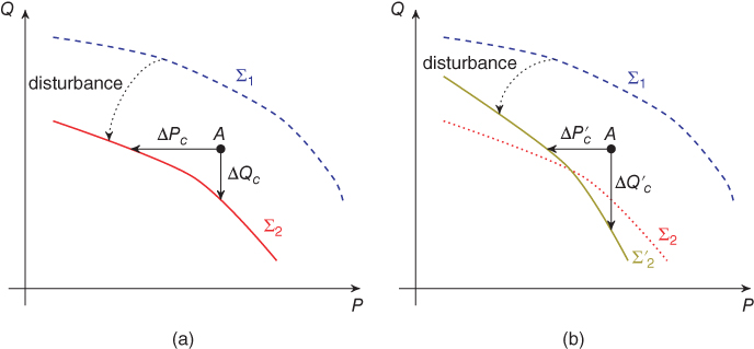
Figure 15.3 Restoration of equilibrium point with corrective actions (a) Curve more sensitive to reactive power (b) Curve more sensitive to active power.
15.2.1 Countermeasures
The main objectives of instability countermeasures are to restore a long-term equilibrium (fast enough so to be in the region of attraction) and stop system degradation. Traditionally, there are several defense mechanisms proposed and applied to achieve these goals, such as reactive compensation switching/boosting, LTC emergency controls, generation rescheduling, and load reduction.
If we assume a load restoration to the pre-disturbance operating point ![]() , the corrective actions need to establish a new operating point inside the feasible region
, the corrective actions need to establish a new operating point inside the feasible region ![]() . From Figure 15.3a, it can be seen that a feasible point can be established by decreasing the load active or reactive power consumption by
. From Figure 15.3a, it can be seen that a feasible point can be established by decreasing the load active or reactive power consumption by ![]() or
or ![]() respectively, or through a combined reduction.
respectively, or through a combined reduction.
Some countermeasures act only in one direction and others in both. For example, reactive compensation reduces the net reactive power consumption; increasing active power generation of local units decreases the net active power consumption seen from the TN; while depressing the DN voltages or shedding some loads decreases both active and reactive power consumption. It can be seen in Figure 15.3a that along each direction there is a different distance to the loadability surface ![]() . Thus, a combination of corrective actions is necessary to achieve the optimal effect.
. Thus, a combination of corrective actions is necessary to achieve the optimal effect.
Moreover, depending on the characteristics of the system after the disturbance, one of the two directions can be more effective than the other. This behavior is shown in Figure 15.3b, where for the feasible region defined by ![]() decreasing the active power consumption is more effective than its reactive counterpart.
decreasing the active power consumption is more effective than its reactive counterpart.
In selection of corrective actions, the impact on consumers should be taken into consideration. Reactive power compensation through shunt switching and generator boosting has no direct adverse effect on customers. Increasing active power generation of local units does not impact customers either, but depends on the available reserves and usually comes at a higher cost. Depressing the DN voltages to exploit Conservation Voltage Reduction (CVR) can be an effective countermeasure but is harmful for consumers if the DN voltages remain uncontrollably low, which may affect or disconnect some appliances such as electronic devices. Finally, when the corrective action to be taken is load shedding, this severely impacts consumers and the amount of load to be shed should be the minimum possible.
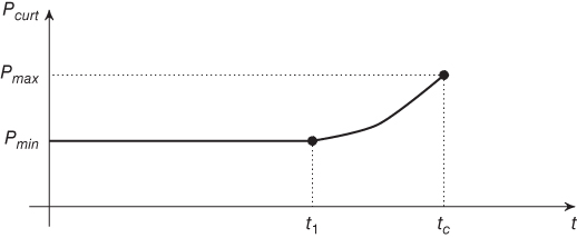
Figure 15.4 Evolution with time of the minimum load curtailment needed to stabilize the system [11].
In addition to defining the type and extent of corrective actions needed, the timing is also of great importance. If the control action is delayed too much then the system may exit the region of attraction rendering the countermeasure useless. Hence, countermeasures with no adverse effect on consumers should be employed as soon as possible while the remainder should be delayed as needed to make sure that they are absolutely necessary. It should be kept in mind though, that the more a countermeasure is delayed, the larger a corrective action could be needed to save the system. For example, Figure 15.4 shows the minimum load reduction needed to save the system as a function of the time to take this action, counted since the disturbance occurrence. Up to a specific time instant, this amount is constant, while after that a larger amount of load needs to be curtailed to save the system. Finally, there is a no-return point in time after which the system cannot be saved.
In this section some basic notions of long-term voltage stability have been introduced, necessary to understanding and analyzing the impact of VVCs at distribution and transmission level. Readers interested in further information concerning this subject can refer to textbooks such as [11, 18].
15.3 Impact of Volt-VAR Control on Long-Term Voltage Stability
In this section we describe how VVC can affect long-term voltage stability. First, we show how incorrectly designed VVCs can precipitate voltage instability. Then, we explain how VVCs can be employed in emergency situations to support the TN.

Figure 15.5 Simple system with DN controlled by LTC and DGUs.
Let us consider the same simple system of Figure 15.1, though now the DN is equipped with a centralized VVC acting on the DGUs, the reactive power compensation devices, the LTC setpoint, and so on. This updated system is sketched in Figure 15.5. While a centralized controller is assumed in this chapter, most of the results derived below can be applied to distributed or local controllers as well.
As discussed in the Introduction, the primary purpose of VVC is to dispatch the available distributed resources to keep the voltages within an acceptable range and alleviate any security problems within the DNs. For example, in case of depressed voltages inside the DN, the VVC will try to support and restore the voltages, usually using reactive power injection from the DGUs or other devices. Similarly, in case of thermal overloads, the VVC will dispatch the DGUs in such way as to alleviate the problem [9], using reactive or even in some instances active power modulation (with dispatchable DGUs, flexible loads, etc.).
Most of the VVC algorithms, either local, distributed, or centralized, assume a strong TN. That is, in their design and testing, stiff transmission voltages are considered. Unfortunately, this hypothesis is no longer valid in degraded operating conditions when interactions between transmission and distribution systems become critical. In such situations, VVCs unaware of the system weakening and operating under the strong TN assumption could end up precipitating the developing voltage instability. Moreover, due to the high speed of action of power-electronic based interfaces (present in many DGUs), the instability could occur much faster than with conventional machines; thus, it becomes harder to detect and apply countermeasures [15].
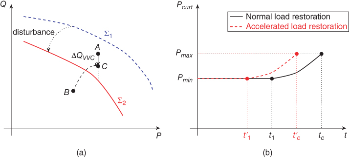
Figure 15.6 Impact of VVCs on long-term voltage stability (a) Disturbance and voltage restoration with VVC (b) Minimum load reduction needed with time after disturbance with effect of VVC.
Let us assume again an incident in the transmission system that causes the loadability curve to shrink, so that point ![]() is left outside the post-disturbance feasible region
is left outside the post-disturbance feasible region ![]() , as shown in Figure 15.6a. The system settles at the short-term equilibrium
, as shown in Figure 15.6a. The system settles at the short-term equilibrium ![]() , inside the post-disturbance feasible region, with a lower load power consumption due to the voltage drop caused by the disturbance. Activated by the depressed voltages inside the DN, the VVC will try to restore the voltages to the pre-disturbance values (
, inside the post-disturbance feasible region, with a lower load power consumption due to the voltage drop caused by the disturbance. Activated by the depressed voltages inside the DN, the VVC will try to restore the voltages to the pre-disturbance values (![]() ) and, assuming a very accurate voltage control with negligible dead-band, will consequently be restoring the load consumption to the pre-disturbance value (point
) and, assuming a very accurate voltage control with negligible dead-band, will consequently be restoring the load consumption to the pre-disturbance value (point ![]() ).
).
The VVC can achieve this voltage restoration by dispatching the DGUs to inject more reactive power. If a total of ![]() is injected into the DN to support the voltages, then a new equilibrium point
is injected into the DN to support the voltages, then a new equilibrium point ![]() is targeted, as shown in Figure 15.6a. Therefore, two mechanisms are working in parallel, the load-voltage restoration increasing the active and reactive power consumption and the VVC increasing the reactive power injection. If the targeted operating point
is targeted, as shown in Figure 15.6a. Therefore, two mechanisms are working in parallel, the load-voltage restoration increasing the active and reactive power consumption and the VVC increasing the reactive power injection. If the targeted operating point ![]() lies within the feasible region defined by
lies within the feasible region defined by ![]() (and VVC acts fast enough to have attraction), then the system will be stabilized by the VVC. Otherwise, this point cannot be reached, and the system will require further corrective actions or it will collapse. Note that in real systems, the situation is more complex as along with the reactive power injection, the system network losses are also modified, thus a positive or negative change in power demand can be observed as well.
(and VVC acts fast enough to have attraction), then the system will be stabilized by the VVC. Otherwise, this point cannot be reached, and the system will require further corrective actions or it will collapse. Note that in real systems, the situation is more complex as along with the reactive power injection, the system network losses are also modified, thus a positive or negative change in power demand can be observed as well.
Furthermore, starting from point ![]() , the VVC accelerates the voltage (and hence the load power) restoration procedure adding to the effect of LTCs. This acceleration is due to the much faster action times of DGUs compared to LTC devices. As explained in the previous section, the timing of applying the necessary corrective actions is important in order to stay within the region of attraction of the feasible point. Thus, by accelerating the voltage restoration procedure, the available time to apply the countermeasures becomes shorter as well, as shown in Figure 15.6b. This behavior can invalidate existing long-term voltage instability countermeasures set in place by transmission system operators.
, the VVC accelerates the voltage (and hence the load power) restoration procedure adding to the effect of LTCs. This acceleration is due to the much faster action times of DGUs compared to LTC devices. As explained in the previous section, the timing of applying the necessary corrective actions is important in order to stay within the region of attraction of the feasible point. Thus, by accelerating the voltage restoration procedure, the available time to apply the countermeasures becomes shorter as well, as shown in Figure 15.6b. This behavior can invalidate existing long-term voltage instability countermeasures set in place by transmission system operators.
15.3.1 Countermeasures
As described in Section 15.2.1, any countermeasure should try to quickly restore a long-term equilibrium and stop system degradation. In addition to the traditional countermeasures described previously, VVCs can be used to restore an equilibrium point by decreasing the net active (resp. reactive) power consumption by ![]() (resp.
(resp. ![]() ), or through a combination of actions. Due to the flexibility of DGUs, DNs equipped with a VVC have higher controllability and, if appropriately designed, they can support the TN in stressed operating conditions [10, 21]. Moreover, VVCs offer a faster way to implement some countermeasures thus avoiding further degradation or loss of attraction due to delays.
), or through a combination of actions. Due to the flexibility of DGUs, DNs equipped with a VVC have higher controllability and, if appropriately designed, they can support the TN in stressed operating conditions [10, 21]. Moreover, VVCs offer a faster way to implement some countermeasures thus avoiding further degradation or loss of attraction due to delays.
As a first action, the reactive power injection of DGUs and other reactive compensation devices controlled by VVC can be used to directly act on ![]() . This is usually a natural response by the VVC when depressed voltages are detected. However, in emergency situations, the objective of strictly controlling the DN voltage profile can be relaxed in favor of supporting the TN voltages through coordinated reactive power compensation [7, 10].
. This is usually a natural response by the VVC when depressed voltages are detected. However, in emergency situations, the objective of strictly controlling the DN voltage profile can be relaxed in favor of supporting the TN voltages through coordinated reactive power compensation [7, 10].
In addition, the VVC can control the active power set-points of DERs to provide ![]() , if these control actions are available in the system. Such devices could be DGUs with the capability of increasing their production, energy storage systems, or even flexible loads that can decrease their consumption. To the same end, some load shedding can be selected as a last option if other methods fail.
, if these control actions are available in the system. Such devices could be DGUs with the capability of increasing their production, energy storage systems, or even flexible loads that can decrease their consumption. To the same end, some load shedding can be selected as a last option if other methods fail.
Finally, VVCs can be used to implement CVR and exploit load voltage reduction providing both ![]() and
and ![]() [15]. Traditionally, load voltage reduction is actuated through a reduction of the voltage set-points of LTCs controlling TN-DN transformers, and acting on a single distribution bus. However, VVCs can be used to complement LTC voltage set-point reduction with coordinated control of DGUs. As the DGUs are located closer to the loads and have faster reaction time than LTCs, they can be used to depress the voltages more effectively and quickly. Furthermore, while an LTC only monitors a single distribution bus, VVC can monitor the voltages inside the entire DN and ensure that a minimum emergency voltage profile is maintained throughout the network.
[15]. Traditionally, load voltage reduction is actuated through a reduction of the voltage set-points of LTCs controlling TN-DN transformers, and acting on a single distribution bus. However, VVCs can be used to complement LTC voltage set-point reduction with coordinated control of DGUs. As the DGUs are located closer to the loads and have faster reaction time than LTCs, they can be used to depress the voltages more effectively and quickly. Furthermore, while an LTC only monitors a single distribution bus, VVC can monitor the voltages inside the entire DN and ensure that a minimum emergency voltage profile is maintained throughout the network.

Figure 15.7 Nordic transmission test system with detailed DNs at six buses.
15.4 Test System Description
In this section, the combined T&D system used to demonstrate the above analysis is detailed (Subsection 15.4.1), along with the VVC used for the control of the DNs (Subsection 15.4.2), and some emergency detection methods employed to activate the support of VVCs to the TN (Subsection 15.4.3).
15.4.1 Test System
To show the notions and techniques analyzed above, a large-scale system is used involving a TN including multiple DNs with dispersed generation. The TN part re-uses the Nordic test system set up by the IEEE PES Task Force on Test Systems for Voltage Stability and Security Analysis [22]. Its one-line diagram is shown in Figure 15.7. It includes 68 buses and 20 synchronous machines modeled with their excitation systems, voltage regulators, power system stabilizers, speed governors, and turbines.
The original TN model included 22 aggregate, voltage-dependent loads behind explicitly modeled TN-DN transformers. Six of them were replaced by 40 detailed distribution systems, behind new TN-DN transformers of smaller powers. The six buses were chosen in the Central area because it is the most impacted by voltage instability.
Each DN is a replica of the same medium-voltage distribution system, whose one-line diagram is shown in Figure 15.8. It consists of eight 11-kV feeders all directly connected to the TN-DN transformer, involving 76 buses and 75 branches. The various DNs were scaled to match the original (aggregate) load powers, while respecting the nominal values of the TN-DN transformers and other DN equipment.
The transformer connecting each DN to the TN is equipped with an LTC controlling its distribution side voltage. To avoid artificial synchronization of transformers, the delays on tap changes were randomized around their original values. Thus, the first tap change takes place 28–32 s after leaving the voltage dead-band and the subsequent changes occur every 8–12 s.
Each DN serves 38 voltage sensitive loads and 15 represented by equivalent induction motors. The voltage sensitive loads are modeled as:

with ![]() (constant current) and
(constant current) and ![]() (constant impedance), respectively.
(constant impedance), respectively. ![]() is set to the initial voltage at the bus of concern, while
is set to the initial voltage at the bus of concern, while ![]() and
and ![]() are the corresponding initial active and reactive powers. The equivalent motors are representative of small industrial motors, with constant torque and a third-order model (the differential states being rotor speed and flux linkages) [18].
are the corresponding initial active and reactive powers. The equivalent motors are representative of small industrial motors, with constant torque and a third-order model (the differential states being rotor speed and flux linkages) [18].
Moreover, it includes 22 DGUs, of which 13 are 3-MVA synchronous generators and the remaining are 3.3-MVA Doubly Fed Induction Generators (DFIGs) [23]. The reactive power of each 3-MVA synchronous generator is adjusted to the value received from the VVC using a local proportional-integral control loop. The latter acts on the set-point of a voltage regulator (responding to faster changes). Similarly, the DFIGs operate in reactive power control mode (see [23]), to meet the power requested by the VVC.
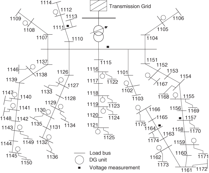
Figure 15.8 Topology of each of the 40 distribution networks.
The combined transmission and distribution model includes 3108 buses, 20 large and 520 small synchronous generators, 600 motors, 360 DFIGs, 2136 voltage-dependent loads, and 56 LTC-equipped transformers.
15.4.2 VVC Algorithm
Each of the 40 DNs is equipped with a separate centralized VVC using the MPC principle. This controller is summarized below and detailed in Chapter 14.
The control variables are the active and reactive power set-points of the DGUs:
where ![]() denotes array transposition and
denotes array transposition and ![]() is the discrete time.
is the discrete time.
At time ![]() , the controller uses a sensitivity-based model to predict the behavior of the system over a future interval with
, the controller uses a sensitivity-based model to predict the behavior of the system over a future interval with ![]() discrete steps (for
discrete steps (for ![]() ):
):
where ![]() is the vector of control changes and
is the vector of control changes and ![]() the one of predicted bus voltages at time
the one of predicted bus voltages at time ![]() given the measurements at time
given the measurements at time ![]() ,
, ![]() is set to the measured values received at time
is set to the measured values received at time ![]() . Matrix
. Matrix ![]() contains the sensitivities of voltages to control variables.
contains the sensitivities of voltages to control variables.
The sequence of control changes optimizes a multi-time step objective under constraints. The following quadratic objective is considered at time ![]() :
:
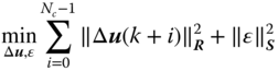
where the squared control changes aim at distributing the effort more evenly over the DGUs and the time steps. ![]() is a weight matrix used to force control priorities. For example, higher costs are assigned to variations of
is a weight matrix used to force control priorities. For example, higher costs are assigned to variations of ![]() compared to
compared to ![]() . The slack variables
. The slack variables ![]() are used when some of the constraints, detailed hereafter, make the optimization problem infeasible. These variables are heavily penalized using the weight matrix
are used when some of the constraints, detailed hereafter, make the optimization problem infeasible. These variables are heavily penalized using the weight matrix ![]() , to keep them at zero when the problem is feasible.
, to keep them at zero when the problem is feasible.
The minimization is subjected to the following inequalities:
The constraints (15.5a) are associated with the permitted range of control variables. The active powers, updated from real-time measurements, are already at their upper limits. The reactive power limits are updated with the voltage and active power as described in [24], based on the information in [25] for the DFIGs. The constraints (15.5b) are associated with the rate of change of control variables. In inequalities (15.5c), ![]() denotes a vector of ones, while
denotes a vector of ones, while ![]() (resp.
(resp. ![]() ) is the desired lower (resp. upper) limit on the voltages. It must be emphasized that voltages are forced to reintegrate their limits at the prediction horizon, that is, at time step
) is the desired lower (resp. upper) limit on the voltages. It must be emphasized that voltages are forced to reintegrate their limits at the prediction horizon, that is, at time step ![]() only.
only.
In principle, the above control scheme is designed to control DN voltages only. The relation of the VVC to TN voltage stability is established by the voltage limits ![]() and
and ![]() set in (15.5c). The selection of these limits can make a difference between reaching a new long term equilibrium point or not, as will be shown in the following sections.
set in (15.5c). The selection of these limits can make a difference between reaching a new long term equilibrium point or not, as will be shown in the following sections.
Measurements involve DGU active/reactive powers and terminal voltages, as well as voltages at three load buses. The latter were selected so that no load is more than two branches away from a voltage monitored bus. The measurement noise was simulated by adding a Gaussian random variable limited to ![]() pu for voltages, and
pu for voltages, and ![]() of the DGU maximum active and reactive powers.
of the DGU maximum active and reactive powers.
15.4.3 Emergency Detection
As discussed in the previous sections, the main objective of VVCs is to keep voltages within some secure limits and to optimize DN operation. To be able to support the TN in emergency situations, some detection mechanisms need to be in place. One such mechanism is LIVES (standing for Local Identification of Voltage Emergency Situations), which was originally proposed in [26]. This mechanism detects the unsuccessful attempt of LTCs to restore their DN voltages, as sketched in Figure 15.2a. To achieve this, LIVES monitors each LTC independently, thus providing a distributed—and more robust—emergency detection mechanism.
Another detection approach is to monitor the reactive reserve of the large, TN-connected generators. It is quite common to have generator reactive power measurements in the SCADA system of TN control centers. A comparison with capability curves can flag a generator that has switched under limit. This information can make up an alternative alarm signal to be send to VVCs, combining simplicity with anticipation capability. This simple emergency detection was used in the simulation reported hereafter.
Table 15.1 Overview of simulated scenarios
 |

Figure 15.9 Simplified loadability curves of considered case studies (a) Case study A (b) Case study B and C.
15.5 Case Studies and Simulation Results
In this section, the case studies used to support the analysis presented earlier in this chapter and their simulation results are shown. Table 15.1 offers an overview of these case studies. They are divided into three groups, namely: stable cases, unstable cases, and unstable cases with the use of emergency corrective actions.
As the timing of controls is critical, long-term dynamic simulations were performed to simulate the system responses to large disturbances in the TN. The simulations were performed with the RAMSES software developed at the University of Liège [27].

Figure 15.10 Cases A1 & A2: voltages at three TN buses.
15.5.1 Results in Stable Scenarios
For these cases, a TN disturbance is considered that is not threatening to the system stability. Thus, the disturbance causes the loadability curve to shrink but the pre-disturbance point ![]() is still within the feasible region, as shown in Figure 15.9a. The disturbance considered is the outage of line 4061-4062 (see Figure 15.7).
is still within the feasible region, as shown in Figure 15.9a. The disturbance considered is the outage of line 4061-4062 (see Figure 15.7).

Figure 15.11 Cases A1 & A2: voltages at two DN buses.
15.5.1.1 Case A1
In this first scenario, the VVCs are not in service. The DGUs operate with constant reactive powers and do not take part in voltage control. This leaves only the traditional voltage control by LTCs. Hence, the DNs are considered passive.
The long-term evolution of the system until it returns to steady state is shown in Figures 15.10 and 15.11. It is driven by the LTCs, in response to the voltage drops initiated by the line tripping. There are some 112 tap changes in all 40 DNs. Figure 15.10 shows the TN voltage evolution at three representative buses of the Central area. The voltage at bus 1041 is the most impacted but remains above 0.985 pu. All DN voltages are successfully restored in their dead-bands by the LTCs, which corresponds to a stable evolution [11]. For instance, Figure 15.11 shows the voltage evolution at two DN buses: 01a, controlled by an LTC with a ![]() pu dead-band, and 01a-1171, located further away in the same DN.
pu dead-band, and 01a-1171, located further away in the same DN.
15.5.1.2 Case A2
The same disturbance as in Case A1 is considered, but the VVCs are now active. For simplicity, all components of ![]() have been set to 0.98 pu and those of
have been set to 0.98 pu and those of ![]() to 1.03 pu. This interval encompasses all LTC deadbands, so that there is no conflict between an LTC and the VVC.
to 1.03 pu. This interval encompasses all LTC deadbands, so that there is no conflict between an LTC and the VVC.
The corresponding TN and DN voltage evolutions can be found in Figures 15.10 and 15.11, for easier comparison. With respect to Case A1, a steady state is reached at almost the same time, while the TN voltages are slightly higher. The voltages at DN buses not directly controlled by LTCs (such as 01a-1171 in Figure 15.11) are restored above ![]() by the VVC.
by the VVC.
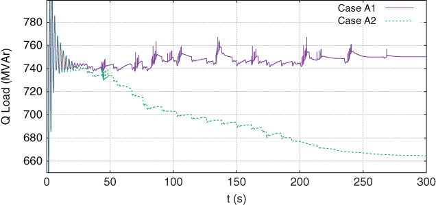
Figure 15.12 Cases A1 & A2: reactive power from TN to DNs.
It is worth mentioning that the number of tap changes has decreased from 112 to 35, showing that the sharing of the control effort by active DNs reduces the wear of LTCs.
The DN buses such as 01a-1171 in Figure 15.11 have their voltages increased by the additional reactive power produced by the coordinated DGUs. For instance, in Case A2, the DG participations decrease the net reactive power load seen by the TN by almost 90 Mvar (see Figure 15.12), which contributes to increasing TN voltages. Note, however, that a hidden effect of this load voltage increase is an increase of active and reactive powers of the voltage sensitive loads. While very moderate in this scenario, this effect will be predominant in the next ones.
15.5.2 Results in Unstable Scenarios
For these cases, a critical TN disturbance is considered leading to long-term voltage instability. The disturbance considered is a 5-cycle short-circuit near bus 4032, cleared by opening line 4032-4042 (see Figure 15.7). First, the disturbance causes the loadability curve to shrink but the pre-disturbance point ![]() is still within the feasible region. Nevertheless, a series of generator OEL actions in the TN further shrink the feasible region leading to a system collapse. This sequence is depicted in Figure 15.9b.
is still within the feasible region. Nevertheless, a series of generator OEL actions in the TN further shrink the feasible region leading to a system collapse. This sequence is depicted in Figure 15.9b.

Figure 15.13 Cases B1 & B2: voltages at two TN buses.
15.5.2.1 Case B1
Similarly to Case A1, in this scenario the DN voltages are only controlled by the LTCs and the VVCs are inactive. The voltage evolutions at two TN buses are shown in Figure 15.13. The sustained voltage sag caused by the LTCs and OELs ends with a system collapse due to the loss of synchronism of machine g6 at ![]() s. The maximum power that can be provided to loads is severely decreased by the initial line outage as well as cascading field current reductions due to seven OELs acting before
s. The maximum power that can be provided to loads is severely decreased by the initial line outage as well as cascading field current reductions due to seven OELs acting before ![]() s. At the same time, the LTCs unsuccessfully attempt to restore DN voltages, which is impossible since load powers cannot be restored at their pre-disturbance values. The static aspects of this mechanism were analyzed in Section 15.2.
s. At the same time, the LTCs unsuccessfully attempt to restore DN voltages, which is impossible since load powers cannot be restored at their pre-disturbance values. The static aspects of this mechanism were analyzed in Section 15.2.
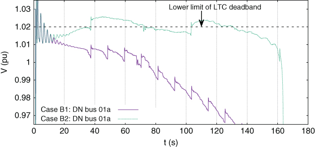
Figure 15.14 Cases B1 & B2: voltage at a DN bus controlled by an LTC.
15.5.2.2 Case B2
In this scenario, in addition to LTCs, the VVCs are also activated. The resulting voltage evolutions can be found in Figures 15.13 and 15.14, while Figure 15.15 shows the total active and reactive powers transferred from the TN to the DNs.

Figure 15.15 Case B2: total active and reactive power transfer from TN to DNs.
Since the DGUs have their reactive power productions increased to correct DN voltages, the net reactive power load seen by the TN decreases progressively, passing from 750 to 200 Mvar in 150 s. This results in TN voltages dropping significantly less than in Case B1, until ![]() s (see Figure 15.13). In principle, this reactive support could prevent voltage instability (see Figure 15.6a), but it is not sufficient in this case, where five OELs are activated successively. The limitations of generator reactive powers are identified in Figure 15.16. At
s (see Figure 15.13). In principle, this reactive support could prevent voltage instability (see Figure 15.6a), but it is not sufficient in this case, where five OELs are activated successively. The limitations of generator reactive powers are identified in Figure 15.16. At ![]() s, soon after the fifth OEL is activated, the system collapses with all generators in the Central and South areas, except g14, going out of step with the rest of the system.
s, soon after the fifth OEL is activated, the system collapses with all generators in the Central and South areas, except g14, going out of step with the rest of the system.
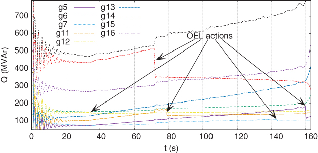
Figure 15.16 Case B2: reactive power produced by TN-connected generators.
This severe outcome is partly explained by the fact that the VVCs promptly restore voltages, and hence, load powers. Consequently, when generators connected to the TN stop controlling their voltages, under the effect of OELs, they are facing a higher load power compared to Case B1. The restoration of DN voltages is illustrated by the dotted curve in Figure 15.14. The voltage is boosted by the controller in significantly less time than with a traditional LTC, with the result that the LTC makes two tap changes only. The resulting fast restoration of load active power is shown in Figure 15.15, where the small, 25-MW non restored power is caused by the (intentional) voltage dead-bands of the controllers.
The overall effect of voltage control at DN level is to precipitate system collapse, while making the latter less predictable from the mere observation of voltages. From a system operation viewpoint, this case is worse than Case B1. The static aspects of this behavior were also explained in Section 15.2.
15.5.3 Results with Emergency Support From Distribution
In this section, Case B is revisited assuming some remedial actions to secure system operation. This requires a timely detection of the emergency condition, which was discussed in Section 15.4.3.
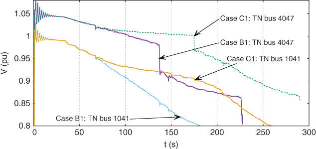
Figure 15.17 Cases B1 & C1: voltages at two TN buses.
The remedial action considered in the sequel is a decrease of DN voltages exploiting the sensitivity of load power to voltage. This effect strongly depends on the type of loads [11, 18, 28]. As long as a decrease in the voltage magnitude leads to decreased load consumption (in active and/or reactive power), the mechanism is beneficial to system stability. However, some loads (for instance induction motors and electronically controlled loads) have the tendency to rapidly restore their consumed power after a voltage decrease. Moreover, induction motors could eventually exhibit increased consumption when approaching their stalling point [18].
The voltage decrease ![]() should be as large as possible while ensuring a minimum acceptable voltage at all DN nodes [28]. When implemented through LTC voltage decrease alone, this reduction is applied at only one point of the DN. This has led system operators to conservatively set
should be as large as possible while ensuring a minimum acceptable voltage at all DN nodes [28]. When implemented through LTC voltage decrease alone, this reduction is applied at only one point of the DN. This has led system operators to conservatively set ![]() to 0.05 pu [11, 18]. On the other hand, acting on multiple DGUs offers better controllability by adjusting DN voltages at multiple points. Therefore, more points of the DN have their voltages decreased while still remaining above the acceptable limit.
to 0.05 pu [11, 18]. On the other hand, acting on multiple DGUs offers better controllability by adjusting DN voltages at multiple points. Therefore, more points of the DN have their voltages decreased while still remaining above the acceptable limit.
Moreover, as the LTC controllers involve mechanical components, their speed of action is limited and can be insufficient to counteract instability. Acting on DGUs offers a significantly faster control of DN voltages.
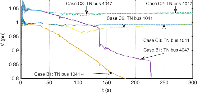
Figure 15.18 Cases B1, C2 & C3: voltages at two TN buses.
15.5.3.1 Case C1
This case involves the classical LTC voltage set-point reduction without any contribution by the VVCs. Thus, this scheme is to be compared to Case B1, from which it differs after ![]() s, when an alarm is received from the generator limitation. At that time, the LTC voltage set-points are decreased by
s, when an alarm is received from the generator limitation. At that time, the LTC voltage set-points are decreased by ![]() pu.
pu.
Figure 15.17 shows the voltage evolution at two TN buses. It can be seen that the amount of load decrease is not enough to stabilize the system. Further tests showed that ![]() pu would be needed. However, in that case, several DN bus voltages are unacceptable, lower than 0.90 pu.
pu would be needed. However, in that case, several DN bus voltages are unacceptable, lower than 0.90 pu.
15.5.3.2 Case C2
Case C2 is to be compared with Case B2, from which it differs after ![]() s, when the generator limitation alarm is received. At that time, the above mentioned
s, when the generator limitation alarm is received. At that time, the above mentioned ![]() corrections are applied. While in the unstable Case C1, the LTCs alone were unable to restore DN voltages, in this case, they contribute, together with VVCs, to depressing the DN voltages.
corrections are applied. While in the unstable Case C1, the LTCs alone were unable to restore DN voltages, in this case, they contribute, together with VVCs, to depressing the DN voltages.
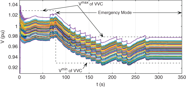
Figure 15.19 Case C2: voltages at various DN buses of the same feeder.

Figure 15.20 Case C2: total active & reactive power transfer from TN to DNs.
Voltage evolutions at TN buses are shown in Figure 15.18, together with those of the uncontrolled Case B1, for comparison purposes. The TN voltages are smoothly stabilized. Figure 15.19 shows the corresponding voltage evolutions in one DN, together with the changing ![]() and
and ![]() limits. It is seen that the DN voltages are promptly brought within the new desired range.
limits. It is seen that the DN voltages are promptly brought within the new desired range.
The voltage reduction causes the decrease of active and reactive power transfer from the TN to DNs, as shown in Figure 15.20. As explained in Section 15.2, the reactive power transferred between the TN and DNs varies with the reactive power produced by the DGUs, the reactive power consumed by the loads, and the network losses. First, the DGUs are directed by the VVCs to reduce and maintain the DN voltages within the emergency limits. To achieve this, they decrease their reactive power productions. Then, the reduced DN voltages lead to decreased reactive power consumption by the loads and decreased losses. In the system studied, the benefit brought by the load decrease outweighs the negative impact of the reduced reactive support from DGUs. Thus, the restored power point is moved as shown in Figure 15.3b, entering the feasible region.

Figure 15.21 Case C2: reactive power produced by TN-connected generators.
The evolution of reactive powers of TN-connected generators for Case C2 is shown in Figure 15.21. It can be seen that no further generator limitation takes place after ![]() s, in contrast to Case B2 where the system eventually collapses after the successive field current limitations of generators g5 and g6, as shown in Figure 15.16. Furthermore, the non-limited generators are relieved, as shown by Figure 15.21.
s, in contrast to Case B2 where the system eventually collapses after the successive field current limitations of generators g5 and g6, as shown in Figure 15.16. Furthermore, the non-limited generators are relieved, as shown by Figure 15.21.

Figure 15.22 Case C2: Effect of time delay on emergency signal.
Effect of time delay in applying the corrective actions
To assess the robustness of the scheme to delays in emergency detection signals, three cases were considered, each with an additional delay of 30 s added to the original alarm time of 75 s. With delays up to 60 s (i.e., with an emergency alarm up to ![]() s), the system can be saved. This is made possible by the fast response of DGUs steered by the VVC. As explained in Section 15.2, there exists a no-return point after which the corrective actions are unable to restore stability as the system has exited the region of attraction, as confirmed by the curves in Figure 15.22.
s), the system can be saved. This is made possible by the fast response of DGUs steered by the VVC. As explained in Section 15.2, there exists a no-return point after which the corrective actions are unable to restore stability as the system has exited the region of attraction, as confirmed by the curves in Figure 15.22.
Sensitivity of CVR-based countermeasure to load types
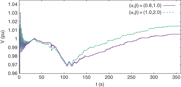
Figure 15.23 Case C2: voltage at a TN bus with two different load model parameter pairs; voltage reduction  pu.
pu.
The emergency technique presented in this Chapter exploits the reduction of load consumption when voltages are decreased. Thus, the sensitivity of loads towards voltage variations is critical to its success. This sensitivity is taken into account through the parameters ![]() and
and ![]() , used in the load model (15.1).
, used in the load model (15.1).
These parameters are selected according to the mixture of loads present in the system. An indicative list can be found in [11, 18]. When the induction motors are modeled explicitly, such as in the test system used, the values ![]() are frequently used.
are frequently used.
These load model parameters determine the load power decrease for a given voltage reduction. Figure 15.23 shows the voltage at a TN bus in Case C3 (![]() pu), with two different sets of parameters. The first pair
pu), with two different sets of parameters. The first pair ![]() is an extreme case, where the loads have very low sensitivity to voltage; while the second is the one used in the simulations previously shown. It can be seen that, even though in both cases the system is saved, with more sensitive loads the voltage recovers a little faster to a higher value.
is an extreme case, where the loads have very low sensitivity to voltage; while the second is the one used in the simulations previously shown. It can be seen that, even though in both cases the system is saved, with more sensitive loads the voltage recovers a little faster to a higher value.
In addition, a parametric study was performed to check the effectiveness of the method as a function of the load model parameters and the emergency voltage reduction (![]() ). Case C2 was considered. The simulation was repeated for several values of
). Case C2 was considered. The simulation was repeated for several values of ![]() (
(![]() pu) and using a wide range of
pu) and using a wide range of ![]() (
(![]() ) and
) and ![]() (
(![]() ) parameter pairs. For
) parameter pairs. For ![]() pu and
pu and ![]() pu, the system is stabilized for all (
pu, the system is stabilized for all (![]() ,
, ![]() ) pairs. For smaller voltage reduction, Figure 15.24 shows the values for which the system can be stabilized.
) pairs. For smaller voltage reduction, Figure 15.24 shows the values for which the system can be stabilized.
According to the plot, in this test system, active power reduction is more effective than its reactive power counterpart. For less sensitive active power loads (lower ![]() values), voltage instability completely depends on
values), voltage instability completely depends on ![]() irrespective of the
irrespective of the ![]() value. As active power load is more sensitivity to voltage,
value. As active power load is more sensitivity to voltage, ![]() starts to have some more importance. Moreover, it is confirmed that, as loads get more voltage sensitive (higher
starts to have some more importance. Moreover, it is confirmed that, as loads get more voltage sensitive (higher ![]() and
and ![]() values), a smaller
values), a smaller ![]() is sufficient to stabilize the system.
is sufficient to stabilize the system.

Figure 15.24 Case C2: regions of successful stabilization in the ( ,
, ) space, for various voltage reduction values
  .
.
15.5.3.3 Case C3
In the last case, we consider the availability of flexible loads inside the DNs. More specifically, in case of emergency, all DNs can defer up to 5% of their original load consumption in increments of 1%. This case can be compared to Case B2.
The VVC controller uses the DGU reactive power to keep the DN voltages within the secure limits as defined in Section 15.4.2. At ![]() s, when the generator limitation alarm is received, the VVCs take a snapshot of their corresponding TN bus voltage and try to stop the degradation by keeping the voltages at that level. To this purpose they decrease their flexible load consumption by 1% at every control action taking place every
s, when the generator limitation alarm is received, the VVCs take a snapshot of their corresponding TN bus voltage and try to stop the degradation by keeping the voltages at that level. To this purpose they decrease their flexible load consumption by 1% at every control action taking place every ![]() s.
s.
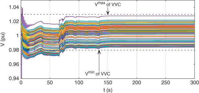
Figure 15.25 Case C3: voltages at various DN buses of the same feeder.
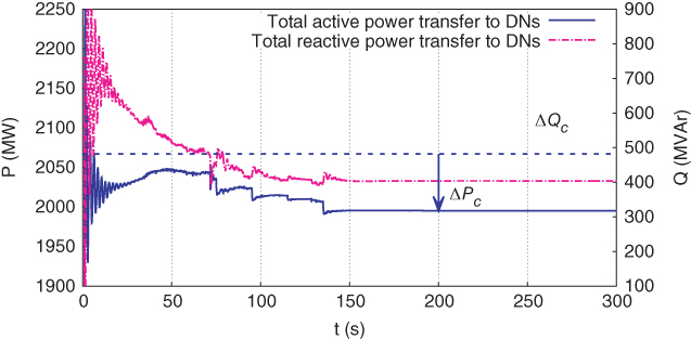
Figure 15.26 Case C3: total active & reactive power transfer from TN to DNs.
The TN voltage evolutions at two buses are shown in Figure 15.18, together with those of the uncontrolled Case B1 and the stabilized using CVR Case C2. The TN voltages are smoothly stabilized. Figure 15.25 shows the corresponding voltage evolutions in one DN. It is seen that the DN voltages are brought within the desired ranges.
The combined corrective actions introduced by the DG reactive power injection and the flexible loads is shown in Figure 15.26. Of course, this power reduction of the flexible loads needs to be restored at a later stage when the system is out of the emergency state (e.g., when the tripped line is reconnected or new generators are put online). However, this procedure is not shown in this chapter.
15.6 Conclusion
This chapter demonstrated how advanced DN control schemes, and in particular Volt-Var Control (VVC), can affect the long-term voltage stability of Transmission Networks (TNs).
Specifically, the chapter has reported on simulations of a large-scale test system including one TN and multiple DNs. The latter are assumed to be active by controlling the reactive power of DGUs, with the aim of keeping DN voltages within a desired range. The DNs are controlled independently of each other, and of the TN. In this study, a specific MPC-based scheme was considered. However, the results are representative of future smart grids in which DGUs will contribute to regulating voltages at other buses than the one controlled by the LTC.
In normal operating conditions, the case study shows some benefits of VVC after a disturbance affecting the TN: (i) by increasing the DGU reactive powers to support DN voltages, the power factor at the TN/DN connection point is improved; (ii) the number of LTC steps is decreased.
On the contrary, in long-term voltage instability scenarios:
- VVC is impacted by the growing weakness of the TN system, which behaves very differently from what is assumed in the VVC scheme, set up for “normal” conditions. The main discrepancy stems from LTCs inability to restore DN voltages as expected.
- VVC control may, in turn, impact system dynamics. This is the case when DGUs are controlled concurrently (and not in complement) to LTCs to restore the DN voltages, and hence the load powers. This fast load power restoration may precipitate system collapse, making the situation more severe than with classical LTC control.
On the other hand, VVC can contribute to corrective actions against voltage instability by decreasing the DN voltages, thereby reducing the power consumed by loads, through the reduction of reactive power production of DGUs. The above action can be triggered:
- either locally, observing the unsuccessful attempt of the LTC to restore its DN voltage, when the VVC is designed to complement LTC operation;
- or centrally, from an alarm signal issued at TN level, when the VVC is set to operate concurrently with the LTC.
References
- 1 Bayod-Rújula, A.A. (2009) Future development of the electricity systems with distributed generation. Energy, 34 (3), 377–383, doi: 10.1016/j.energy.2008.12.008.
- 2 Lopes, J.P., Hatziargyriou, N.,Mutale, J., Djapic, P., and Jenkins, N. (2007) Integrating distributed generation into electric power systems: A review of drivers, challenges and opportunities. Electric Power Systems Research, 77 (9), 1189–1203, doi: 10.1016/j.epsr.2006.08.016.
- 3 Joos, G., Ooi, B., McGillis, D., Galiana, F., and Marceau, R. (2000) The potential of distributed generation to provide ancillary services, in 2000 Power Engineering Society Summer Meeting (Cat. No.00CH37134), vol. 3, IEEE, vol. 3, pp. 1762–1767, doi: 10.1109/PESS.2000.868792.
- 4 Kulmala, A., Repo, S., and Järventausta, P. (2014) Coordinated voltage control in distribution networks including several distributed energy resources. IEEE Transactions on Smart Grid, 5 (4), 2010–2020, doi: 10.1109/TSG.2014.2297971.
- 5 Agalgaonkar, Y.P., Pal, B.C., and Jabr, R.A. (2014) Distribution voltage control considering the impact of pv generation on tap changers and autonomous regulators. IEEE Transactions on Power Systems, 29 (1), 182–192, doi: 10.1109/TPWRS.2013.2279721.
- 6 Ranamuka, D., Agalgaonkar, A.P., and Muttaqi, K.M. (2016) Online coordinated voltage control in distribution systems subjected to structural changes and dg availability. IEEE Transactions on Smart Grid, 7 (2), 580–591, doi: 10.1109/TSG.2015.2497339.
- 7 Valverde, G. and Van Cutsem, T. (2013) Model predictive control of voltages in active distribution networks. IEEE Transactions on Smart Grid, 4 (4), 2152–2161, doi: 10.1109/TSG.2013.2246199.
- 8 Soleimani Bidgoli, H., Glavic, M., and Van Cutsem, T. (2014) Model predictive control of congestion and voltage problems in active distribution networks, in Proc. CIRED conference, paper No 0108.
- 9 Soleimani Bidgoli, H., Glavic, M., and Van Cutsem, T. (2016) Receding-horizon control of distributed generation to correct voltage or thermal violations and track desired schedules, in Proc. 19th Power Systems Computation Conference (PSCC), Genoa, Paper. No. 114, p. 7.
- 10 Valverde, G. and Van Cutsem, T. (2013) Control of dispersed generation to regulate distribution and support transmission voltages, in Proceedings of IEEE PES 2013 PowerTech conference, doi: 10.1109/PTC.2013.6652119.
- 11 Van Cutsem, T. and Vournas, C. (1998) Voltage Stability of Electric Power Systems, Springer.
- 12 Vournas, C. and Karystianos, M. (2004) Load tap changers in emergency and preventive voltage stability control. IEEE Transactions on Power Systems, 19 (1), 492–498, doi: 10.1109/TPWRS.2003.818728.
- 13 Vournas, C., Metsiou, A., Kotlida, M., Nikolaidis, V., and Karystianos, M. (2004) Comparison and combination of emergency control methods for voltage stability, in 2004 IEEE Power Engineering Society General Meeting, vol. 2, IEEE, vol. 2, pp. 1799–1804, doi: 10.1109/PES.2004.1373189.
- 14 Hiskens, I.A. and Gong, B. (2006) Voltage stability enhancement via model predictive control of load. Intelligent Automation & Soft Computing, 12 (1), 117–124, doi: 10.1080/10798587.2006.10642920.
- 15 Aristidou, P., Valverde, G., and Van Cutsem, T. (2015) Contribution of distribution network control to voltage stability: A case study. IEEE Transactions on Smart Grid, pp. 1–1, doi: 10.1109/TSG.2015.2474815.
- 16 Crider, C. and Hauser, M. (1990) Real time t&d applications at virginia power. IEEE Computer Applications in Power, 3 (3), 25–29, doi: 10.1109/67.56579.
- 17 Wang, Z. and Wang, J. (2014) Review on implementation and assessment of conservation voltage reduction. IEEE Transactions on Power Systems, 29 (3), 1306–1315, doi: 10.1109/TPWRS.2013.2288518.
- 18 Taylor, C.W. (1994) Power System Voltage Stability, Mc Graw Hill.
- 19 Löf, P.A., Hill, D.J., Arnborg, S., and Andersson, G. (1993) On the analysis of long-term voltage stability. International Journal of Electrical Power & Energy Systems, 15 (4), 229–237, doi: 10.1016/0142-0615(93)90022-F.
- 20 Dobson, I. and Lu, L. (1993) New methods for computing a closest saddle node bifurcation and worst case load power margin for voltage collapse. IEEE Transactions on Power Systems, 8 (3), 905–913, doi: 10.1109/59.260912.
- 21 ENTSO-E (2012) Network code on demand connection, Tech. Rep. URL https://www.entsoe.eu.
- 22 IEEE PES Task Force (2015) Test system for voltage sability analysis and security assessment, Tech. Rep., PES-TR19.
- 23 Ellis, A., Kazachkov, Y., Muljadi, E., Pourbeik, P., and Sanchez-Gasca, J. (2011) Description and technical specifications for generic WTG models: A status report, in Proc. IEEE PES 2011 Power Systems Conference and Exposition (PSCE), doi: 10.1109/PSCE.2011.5772473.
- 24 Valverde, G. and Orozco, J. (2014) Reactive power limits in distributed generators from generic capability curves, in Proc. IEEE PES 2014 General Meeting.
- 25 Engelhardt, S., Erlich, I., Feltes, C., Kretschmann, J., and Shewarega, F. (2011) Reactive power capability of wind turbines based on doubly fed induction generators. IEEE Transactions on Energy Conversion, 26 (1), 364–372, doi: 10.1109/TEC.2010.2081365.
- 26 Vournas, C. and Van Cutsem, T. (2008) Local identification of voltage emergency situations. IEEE Transactions on Power Systems, 23 (3), 1239–1248, doi: 10.1109/TPWRS.2008.926425.
- 27 Aristidou, P., Fabozzi, D., and Van Cutsem, T. (2014) Dynamic simulation of large-scale power systems using a parallel Schur-complement-based decomposition method. IEEE Transactions on Parallel and Distributed Systems, 25 (10), 2561–2570, doi: 10.1109/TPDS.2013.252.
- 28 Wang, Z. and Wang, J. (2014) Review on implementation and assessment of conservation voltage reduction. IEEE Transactions on Power Systems, 29 (3), 1306–1315, doi: 10.1109/TPWRS.2013.2288518.