Chapter 2
Steady-State Security
Evelyn Heylen1, Steven De Boeck1, Marten Ovaere2, Hakan Ergun1 and Dirk Van Hertem1
1Research group ELECTA, Department of Electrical Engineering, University of Leuven, Belgium
2Department of Economics, University of Leuven, Belgium
The power system can be seen today as one of the most critical infrastructures. The reliability of the power system influences the economics and social well-being of a modern society and has a direct impact on the quality of life. A one day blackout could lead to costs that are about 0.5% of the GDP of a country, which have to be added to possible social consequences of longer interruptions, such as diseases, deaths and injuries [1]. Also short term interruptions cause loss of production, frozen foods gone bad, traffic accidents, and so on. Moreover, the reliability of local energy provisions might be key to the selection of an industrial site, which is important for particular industries such as foundries and large IT providers.
Power system reliability is managed in order to minimize the impact to society. Ideally, the achieved power system reliability represents the optimal balance between the value of reliability and its cost. In practice, an “adequate level of reliability” is aimed for [2]. In order to obtain an adequate reliability level, appropriate actions can be taken throughout the lifetime of the power system, from years ahead (i.e., system development) up to real time (i.e., operation). These actions are the result of power system reliability management based on a well defined reliability criterion.
Power system reliability is determined by the existence of sufficient facilities in the system to satisfy the electrical power requirements of consumers at all times and by the system's ability to handle disturbances arising in the system. The latter is also defined as power system security and will be the main topic of this chapter. The focus is on steady-state security.
Section 2.1 introduces power system reliability management, while Section 2.2 explains the challenges due to uncertainties in reliability management in different timeframes ranging from long-term system development up to short-term system operation. Section 2.3 goes more into the shortcomings of currently used reliability criteria, while Section 2.4 elaborates on the socio-economic evaluation of power system reliability management considering the trade-off between the cost of reliability management and interruption costs. Section 2.5 concludes the chapter.
2.1 Power System Reliability Management: A Combination of Reliability Assessment and Reliability Control
Power system reliability is defined as the probability that an electrical power system can perform a required function under given conditions for a given time interval [3]. It quantifies the ability of a power system to provide an adequate supply of electrical energy in order to satisfy the customer requirements with few interruptions over an extended period of time. The degree of reliability is measured by the frequency, duration and magnitude of the adverse effects on consumer service [4].
Power system reliability consists of power system security and power system adequacy [4]. An adequate power system has sufficient generating, transmission and distribution facilities in the system to satisfy the aggregate electric power and energy requirements of customers at all times, taking into account scheduled and unscheduled outages of the system components [4]. System security on the other hand describes the ability of the system to handle disturbances, such as the loss of major generation units or transmission facilities [4]. Sudden disturbances in power systems may result from factors external to the system itself, such as weather and environment, or internal factors such as insulation failure or failure of a plant item [5]. Power system security and adequacy are strongly interdependent, because adequacy is subject to transitions between different states, which are strictly not part of adequacy analysis but of security analysis [6].
Power system reliability expresses whether the system is able to fulfil its required function. It depends on the system's vulnerability to external threats that can lead to unwanted events and the expected function of the system specified by the reliability criterion. The reliability criterion imposes a basis to determine whether or not the power system is managed in an adequate and secure way. The vulnerability of a power system is an expression of the problem the system faces to maintain its function if a threat leads to an unwanted event and the problems the system faces to resume its activities after the event occurred. It is an internal characteristic of the system and is composed of its susceptibility to external threats and its coping capacity. The power system is susceptible to a threat if a realization of the threat leads to an unwanted event in the power system [7]. The coping capacity describes the ability of the operator and the power system itself to cope with an unwanted event, limit negative effects and restore the power system's function to a normal state [8]. It is determined by the adequacy and the security of the system. Criticality of unwanted events, such as power system failure, represents consequences for end-users, such as generators, consumers, traders, suppliers, and so on. [7]. The interaction between vulnerability and reliability with their different aspects and the reliability criterion is graphically shown in Figure 2.1.

Figure 2.1 Interactions between the aspects determining reliability of power systems.
Power system reliability management aims to serve load with a very high probability and this at the required quality and with a very low frequency of experiencing spectacular system failures such as blackouts [4]. Nowadays, reliability is mainly managed according to the N–1 criterion.1 The power system reliability management process of transmission system operators is illustrated graphically in Figure 2.2. It consists of two main tasks: (i) reliability assessment and (ii) reliability control. Reliability assessment aims at identifying and quantifying the actual reliability level, while reliability control consists of taking a sequence of decisions under uncertainty that satisfy the reliability criterion, while minimising the socio-economic costs of doing so.
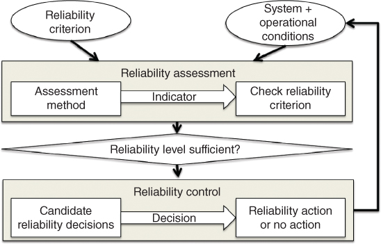
Figure 2.2 Overview of reliability management.
2.1.1 Reliability Assessment
Reliability assessment methods allow verification of whether reliability criteria are satisfied and to quantify the reliability of the system in terms of reliability indicators based on frequency, duration or probability of malfunctioning. The two main reliability assessment methods are analytical contingency enumeration and simulation techniques, such as Monte Carlo simulation [10, 11]. Advantages and disadvantages of both techniques are summarized in Table 2.1. Due to the deterministic nature of currently used reliability criteria, contingency enumeration is mostly applied nowadays. Operational limit violations of system variables are verified for a predefined set of contingencies. Probabilistic security assessment on the other hand should in theory assess all possible system states with their respective probability. This is not possible in practice, especially not in large systems. Alternatively, simulation techniques, such as Monte Carlo simulation, can be used for probabilistic reliability assessment [6]. Hybrid techniques combine aspects of both approaches [12].
Table 2.1 Advantages and disadvantages of methods for steady-state security assessment
| Analytical | Simulation (Monte Carlo) |
| System represented as mathematical model | Simulate actual process and random behavior of the system |
| Mathematically complex | Higher computation time |
| Focus on expected values | Information about underlying distributions |
| State selection: Probability-based or order of contingency level | State selection: Probability-based random numbers |
Reliability assessment is a combination of security assessment and adequacy assessment. Adequacy assessment verifies whether the system is capable of supplying the load under specified contingencies without operating constraint violations. Power system security assessment on the other hand determines whether the immediate response of the system to a disturbance generates potential reliability problems [13]. A distinction can be made between dynamic (time-dependent) and static or steady-state (time-independent) security assessment, depending on whether transients after the disturbance are neglected or not. Steady-state security assessment should evaluate whether a new equilibrium state exist for the post-contingency system, while dynamic security assessment investigates the existence and security level of the transient trajectory in the state space from the original pre-contingency equilibrium point to the post-contingency equilibrium point. The power system model in dynamic security assessment is given by non-linear differential equations whose boundary conditions are given by the non-linear power flow equation. Static security can be considered as a first-order approximation of the dynamic power system state [14]. Alternatively, pseudo-dynamic evaluation techniques using sequential steady-state evaluation to assess the impact at several post-contingency stages exist [15].
2.1.2 Reliability Control
To be able to provide the desirable level of reliability, the power system needs to be able to cope with a certain number of contingencies. In current practice, power systems are designed and operated to withstand a number of “credible” contingencies. If the N–1 criterion is applied, the list of credible contingencies consists of all contingencies in which one component or no components are out of service. During the reliability assessment, the state of the power system is determined. Based on that state, the reliability control mechanism selects a reliability decision from the list of candidate decisions. Decisions imply either a reliability action or no action. Executed reliability actions aim to change the state of the system such that the reliability criterion is satisfied and system security is ensured. Ideally, reliability control performs these actions while minimizing total system cost. Available reliability actions depend on the time horizon considered.
2.1.2.1 Credible and Non-Credible Contingencies
A credible contingency is a disturbance which has been specifically foreseen in the planning and operation of the power system, and against which specific measures have been taken to ensure that limited consequences would follow its occurrence [5]. In general, a contingency is considered as the trip of one single or several network elements that cannot be predicted in advance [16]. A scheduled outage, such as outage of a line for maintenance, is not classified as a contingency. In continental Europe, a further subdivision of credible contingencies is made to distinguish between “normal contingencies” and “exceptional contingencies,” as is depicted in Figure 2.3 [16]. Based on the currently used N–1 framework, the normal contingency is the loss of a single network element. Exceptional contingencies consist of single events that effect multiple network components, for example the falling of a tower resulting in the loss of a double circuit line. Each transmission system operator determines, based on its own risk assessment, which exceptional contingencies are included in the contingency list in order to prevent cascading events. A system that is able to maintain all system parameters within acceptable limits for each of the contingencies on this contingency list is considered to be N–1 secure. On the other hand we have non-credible contingencies, which are often also described as out-of-range or high impact low probability contingencies. These are rare contingencies that often result from exceptional technical malfunctions, force majeure conditions, common mode failures or human errors [17]. As well as being rare, out-of-range contingencies vary significantly with respect to their causes and consequences and thus are hardly ever predictable. Often they are accompanied by the removal of multiple components, cascading of outages and loss of stability leading to a wide area impact. As such these out-of-range contingencies, as well as a sequence of normal contingencies, pose a real threat to power system security [18, 19].
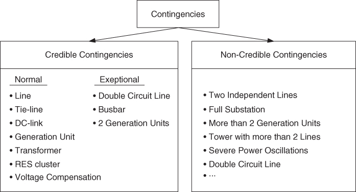
Figure 2.3 Typical categorization of contingency ranking in continental Europe.
2.1.2.2 Operating State of the Power System
The condition the power system is operating in can be subdivided into a number of different operating states, describing the health of the system. The operating state is a concise statement on the viability of the system in its current operating mode [5]. A given operating state can be seen as the collection of system states (combinations of generation, load and grid settings) for which that operating mode is valid. Depending on the state in which the system is operating, the operator manages the system in a particular manner. In order to operate the system securely, it is important to correctly identify the operating state. Due to different events in the system, for example a contingency, the state of the power system can deteriorate. Based on the current state, the expected state of the system and possible future contingency states, the operator will undertake control actions. In an interconnected power system, it is of utmost importance that each system operator communicates the operating state of their area, certainly when not operating in the normal state. Depending on the interconnected area, different classifications have been agreed to. The classification which has been adopted here is the classification of continental Europe. In this classification, a distinction is made between four different states, namely: normal, alert, emergency and blackout state [20, 21]. The security criterion used is the well-known N–1 criterion.
- Normal: The system is considered to be in the normal state when all the system parameters (frequency, voltages, thermal loadings) are within secure operational limits and following any event of the contingency list, taking into account effects of predefined remedial actions, all operational criteria are still fulfilled. The system is operating within its security criterion. The system is said to be operating N–1 secure.
- Alert: All system parameters are still within secure operational limits, but at least for one contingency state, the security criterion (e.g., N–1 security) cannot be maintained. The system is still in a secure state. In case of occurrence of a contingency, it is uncertain whether the system can come back to the normal or alert state. Neighboring systems potentially endure a significant risk. Corrective actions are required without delay in order to comply with the reliability criterion. In case such actions are not available, the system may enter into a more dangerous state once the system operating conditions change. This change can arise from a new contingency or the gradual change of system variables such as load or generation.
- Emergency: The system is strongly disturbed and system parameters are no longer within secure operational limits. As such, the power system state is not viable and without timely intervention will result in full or partial system collapse. Available and prepared actions are undertaken immediately without guarantee of total efficiency to limit propagation to neighboring systems. These actions are defined in the defense plan and strive to avoid full system collapse and to limit the risk of spreading disturbances to other parts of the system or the neighboring systems. These actions can be manual or automatic. The automatic actions are often described in special system protection schemes and try to maintain the integrity of the backbone of the power system. As a result of these emergency actions, it is likely that part of the system is islanded or even disconnected. In this case, system integrity is not maintained and restoration is needed.
- Blackout: This state is characterized by almost total absence of voltage in a certain area of the transmission system as a consequence of the tripping or islanded operation of generating units due to abnormal variations of voltage and/or frequency which occurred during an emergency state. The blackout can be partial (only part of the system is affected) or total (the whole system is affected).
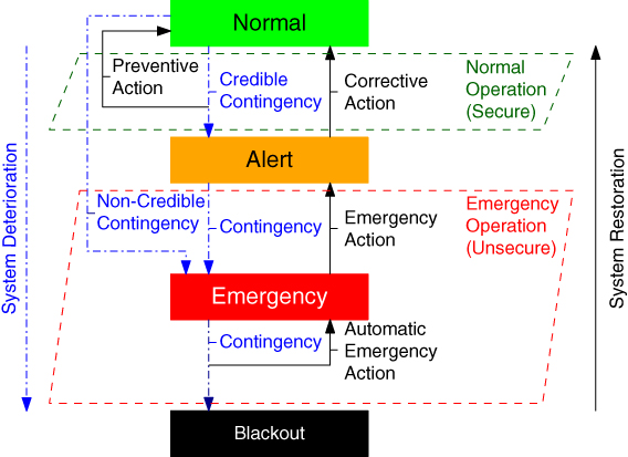
Figure 2.4 Power system in states.
The different states of the power system are shown in Figure 2.4. The transition between the different states can lead either to system deterioration or to system restoration. System deterioration is the sequence of contingencies that lead to the transition from normal to a less secure state (alert, emergency) or even blackout. This process can be halted by either manual or automatic control actions.
During normal operation, the system is operated to meet accepted security and reliability standards at a cost as low as possible, while making provisions to guarantee future operation [5]. The speed associated with these control actions is of relatively low importance. For these remedial actions, distinction can be made between preventive and corrective actions. A preventive action is launched prior to the occurrence of the contingency. This to anticipate the need that may occur due to the uncertainty to cope with the contingency effectively, within the given time span resulting from the system constraints. This action ensures additional margin to the security boundary. The preventive actions will impose a cost, even though it is unsure whether the contingency will take place and hence whether the margin was required. The preventive controls will avoid the system going beyond system limits as long as only considered contingencies occur. For the N–1 criterion, this means that the power system controls are set such that no security boundary is violated after the outage of any single credible contingency. Rather, a corrective action is activated after the occurrence of the contingency. Typically this only imposes a cost once the contingency takes place (activation), unless reservation costs are required (e.g., keeping generation capacity on hot standby). As such the corrective actions realizes the transition from the alert state to the normal state.
Emergency operation consists of actions undertaken to prevent further system degeneration and to halt this process in the alert or emergency state. In general, the cost of these operations is of secondary consideration, as it is of utmost importance to return to normal operation as quickly as possible, even if only for a part of the system, and to avoid system collapse. This set of emergency actions, which are collected in the defense plan, can be both manual or automatic, depending on the type of phenomena and magnitude of the operational limit violation. In general, the defense plan includes a set of coordinated and mostly automatic measures to ensure fast reaction to large disturbances and to avoid their propagation through the system [22].
Once part of the system enters the blackout state, the restoration plan is initiated. The restoration plan aims to reduce the duration of power system interruptions by reenergizing the backbone transmission system as fast as possible, to allow gradual reconnection of generating units and, subsequently, supply to customers. Prompt and effective power system restoration is essential for the minimization of downtime and costs to the utility and its consumers.
A full blackout due to a foreseen power imbalance can be avoided using rolling blackouts. During these rolling blackouts, the electricity supply will be intentionally switched off in indicated areas for a fixed time period. An alternative for small power imbalances are brownouts, which are deliberate decreases of system voltage for a short period of time to avoid rolling blackouts.

Figure 2.5 State space representation of system states. (a) Limited uncertainty (b) Increased uncertainty.
2.1.2.3 System State Space Representation
An abstract visualization of the system states is provided by the system state representation in Figure 2.5 [23]. In this visualization, the current system operation point is depicted relative to the different security borders defined by each of the states. The current operation point is indicated by the point A and is the result of all the input and control variables and parameters present in the power system. The position of the operation point in this state space representation depends on the active power injections and off take ![]() , the reactive power injections and off take
, the reactive power injections and off take ![]() , the set points of the phase shifting transformers (
, the set points of the phase shifting transformers (![]() ) and the set points of the HVDC connections in the system (
) and the set points of the HVDC connections in the system (![]() and
and ![]() ). As most of these input variables are continuously subjected to small changes such as load and generated power variations, the operating point is continuously moving in an uncertainty cloud (Figure 2.5a). In the traditional power system, vertically integrated and mainly depending on fully controllable generation, this uncertainty cloud was relatively small and mainly characterized by load variations. However, due to power system unbundling and ongoing integration of more renewable generation sources, the uncertainty has increased. Now, both generation and load variations are bigger and interdependent with the power market and weather conditions. As can be seen in Figure 2.5b, even though the operating point obtained during steady state power system analysis was considered to be in the normal operating space, these variations lead to a more likely transition into the alert or even emergency state. Depending on how the system is managed, this is usually addressed by adding an additional reliability margin.
). As most of these input variables are continuously subjected to small changes such as load and generated power variations, the operating point is continuously moving in an uncertainty cloud (Figure 2.5a). In the traditional power system, vertically integrated and mainly depending on fully controllable generation, this uncertainty cloud was relatively small and mainly characterized by load variations. However, due to power system unbundling and ongoing integration of more renewable generation sources, the uncertainty has increased. Now, both generation and load variations are bigger and interdependent with the power market and weather conditions. As can be seen in Figure 2.5b, even though the operating point obtained during steady state power system analysis was considered to be in the normal operating space, these variations lead to a more likely transition into the alert or even emergency state. Depending on how the system is managed, this is usually addressed by adding an additional reliability margin.
The outer black line in Figure 2.5 represents the security threshold of the system. This is the theoretical limit, determined by all the security limits (boundary conditions) of the system. Such security limits can consist of the thermal limits of the branches in the system, the voltage and transient stability limits. In theory, it is possible to operate the system up to this threshold without directly resulting into a loss of load or even a blackout. The space outside this region is unsecured, and sustained operation in this space will eventually lead to partial or full system collapse as some of the systems operating limits are violated. As such these operating points are not steady state secure. The space confined by the dashed line is the space defined by the N–1 criterion, or any other reliability criteria in use by the operator. It represents the boundary between the normal state and the alert state. During normal operation, the operating point can temporarily shift between normal and alert space. However, the operator tries to maintain the operating point in the normal space. The alert state results in an operating point between the dashed and full line. The state space should not be considered to be static, as both the boundary conditions and the operating point change continuously. However, each of the operating points in the secure space can be considered as steady-state-secure. In general, the operator tries to maximize the distance between the operating point and the secure threshold, which can be considered as the security margin. But simultaneously all stakeholders of the power system, including system operators, try to make optimal use of the system and minimize generation and operation cost; this typically moves the operating point in the direction of the security margin.
A credible contingency can either result in a change of operating point or a change of a system limit. In Figure 2.6 the tripping of a transmission line is depicted, which causes a reduction of the secure space. As a consequence, the operating point may shift into the alert space as the normal state space is reduced. At this point, the system operator has a number of possible corrective actions to bring the system to a more secure state. A first option is the re-dispatch of generation or the use of flexible demand, which causes the operation point to move away from the secure threshold to a more secure location. A second solution consists of topology changes (line or busbar switching), which can enlarge the secure space near the operating point and can increase the distance between this point and the secure threshold. Thirdly, as more and more controllable devices (phase-shifting transformers, HVDCs) are being integrated into the power system, changing the set points of power flow controllable devices may shift the operation point to the normal state space. All possible actions come at a cost and have a certain effectiveness in influencing the operating point. Depending on the available resources and their cost, the system operator chooses the most appropriate action, either as a preventive action, or as a corrective action.
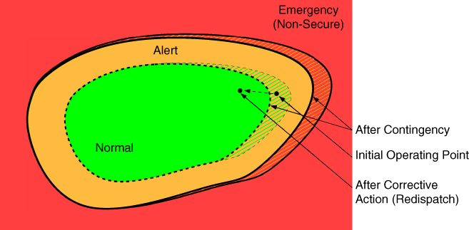
Figure 2.6 Line outage in state space representation.
In Figure 2.7, the effect of a generation outage is shown in the state space representation. An outage of a generator results in a change in input variables and can shift the operating point into the alert state. After this outage, several corrective actions (re-dispatch, load disconnection, etc.) remain available to the operator to bring the system back to the normal state. After activation of the corrective action, the operating point is shifted back to the normal state as depicted in Figure 2.7. In practice, the outage of a generator is proactively managed by the operator through preventive actions, such as system topology changes.
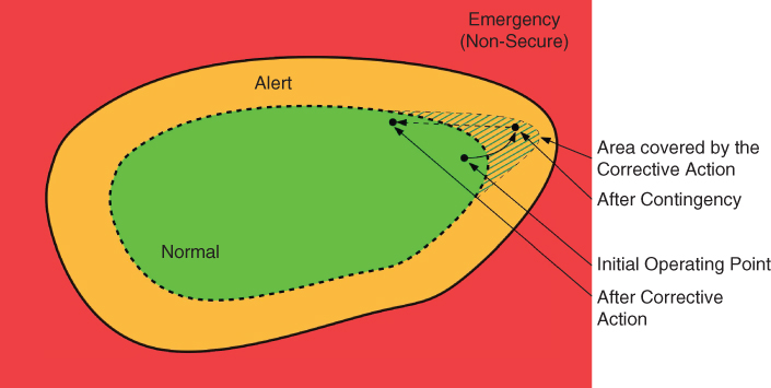
Figure 2.7 Generation outage in state space representation.

Figure 2.8 The uncertainty space in various timeframes.
2.2 Reliability Under Various Timeframes
The level of uncertainty in system operation increases with increased distance to actual operation. As such, the system planner is faced with substantially larger uncertainties than the operator in the control room (Figure 2.8). Both the state of the grid and the generation and load injections in the system are more uncertain. At the same time, the system planner has more possibilities to accommodate the future power system (e.g., building new transmission lines), while the operator in the control room can only use that equipment which is available at that moment. Investment plans and operational decisions taken by system operators are driven by the uncertainty space the operator perceives at the time of planning. Because of these differences, reliability management is performed differently in the different timeframes. In order to deal with the uncertainty and avoid potentially operating in an operating state with insufficient system reliability, system operators usually define either a set of extreme cases or analyze a large number of operating states and contingencies.
The traditional approach to long-term system design is to define maximum and minimum system load cases and apply a fixed set of contingencies to these extreme cases. While there is a higher uncertainty due to more volatile power flows from renewable generation, computational speed has improved significantly. As a consequence, most system operators have moved toward analysis of a larger set of generation and demand samples in order to find more accurate boundaries for the system state space. New investments and topological changes to the system are based on planning cases using these generation and demand samples. This helps system operators to achieve cost savings in long-term system design as well as daily operation, while better covering the uncertainty space around nodal generation and demand values. During system planning, the analysis is mainly focused on active power flows.
The generation and demand samples used by the system operator typically differ between investment and operational planning, both in number of samples used, the granularity involved and the actual values of these samples. As the planning time horizon reduces, more information becomes available and the uncertainty around the system state reduces. This allows the operator to make better guesses of where the borders of the system state will be. This also means that the actions taken closer to real time are in general better fitted to addressing the reliability of the system. Close to real time, the operator usually has fewer control actions at their disposal and less time to evaluate and to decide which actions to take in case of contingencies. As a consequence, the operator chooses to operate the system in a state with sufficient security margin. This is done through the use of preventive actions, using corrective actions only if necessary, resulting in higher operational costs.
The number of possible contingencies in a power system scale exponentially with the number of considered elements. For instance, in a system with 10 elements, ![]() different combinations of outages, thus contingencies, exist. In long term and operational planning, the system is designed to be functional for a specific set of contingencies as the computation of all possible contingencies is not feasible. Hence, the set of contingencies needs to be defined very carefully, as it is a design parameter in the long term and a limiting factor during operation. System operators commonly use the
different combinations of outages, thus contingencies, exist. In long term and operational planning, the system is designed to be functional for a specific set of contingencies as the computation of all possible contingencies is not feasible. Hence, the set of contingencies needs to be defined very carefully, as it is a design parameter in the long term and a limiting factor during operation. System operators commonly use the ![]() criterion, assuming that all contingencies have the same probability of occurrence. This usually leads to an overestimation of the risk as not all contingencies have the same probability of occurrence or the same consequence. The most commonly used reliability criterion is the N–1 criterion, with
criterion, assuming that all contingencies have the same probability of occurrence. This usually leads to an overestimation of the risk as not all contingencies have the same probability of occurrence or the same consequence. The most commonly used reliability criterion is the N–1 criterion, with ![]() chosen as 1.
chosen as 1.
A more cost-effective approach to system operation with regard to reliability is the application of dynamic contingency sets. Using dynamic contingency sets, the analyzed contingencies are updated over time as more information about the operating states of the system becomes available. For example, in long-term planning, the contingencies can be selected based on the contingency probability, as the uncertainty around the operating state is high and the estimation of the consequence more difficult. Closer to real-time operation, the contingency set can be narrowed down and reconstructed using the expected impact of the contingencies, given that the uncertainty around the operational state will have reduced.
2.3 Reliability Criteria
The first reliability criteria used in practical applications, and still used nowadays, are deterministic in nature. The currently used criteria are typically derived from the deterministic N–1 criterion, which states that at any moment, the system should be able to withstand the loss of any one of its main elements (lines, transformers, generators, etc.) without significant degradation of service quality. The N–1 criterion and its derivates, however, have various shortcomings [1, 10, 24–27]:
- They can be interpreted in many ways. In practice, neither the number of elements to be considered (“N”) nor the type of contingencies considered (“−1”) is dealt with equally amongst system operators, or even within a single organization.
- Different contingencies are assumed to be equally severe and equally likely to occur.
- They do not give an incentive based on economic principles, as they do not take outage costs into account.
- All grid elements are assumed equally important and all generators and consumers have equal weight.
- They do not consider the stochastic nature of failures of grid components, generation and demand, the interdependencies between different events or the interaction between the frequency of the contingencies and the exposure time to high stress conditions.
- They are binary criteria: the system is either reliable or not reliable. Therefore, an accurate reliability level cannot be obtained. This results in over- or under-investments and operating costs that do not correspond with the required reliability requirements.
- They only take into account single contingencies. Single contingencies are much more probable than simultaneous contingencies if the outages are independent events. Nevertheless, simultaneous contingencies are not impossible. For example, hidden failures in the protection system can trigger additional outages, in addition to the original fault. Furthermore, due to the significant increase in the rate of outages during bad weather conditions, the probability of two quasi-simultaneous but independent outages may no longer be negligible.
Nevertheless, N–1 criteria, or adapted formulations of the N–1 criterion, are still commonplace, and this for various reasons. Operational experiences using these methods have been very good, due to the predictability and controllability of electrical power system operation and the experience of the system operator. Interconnections were initially aimed at reducing risks in terms of short-term adequacy, while keeping cross-border flows limited in normal operation. N–1 criteria could be easily satisfied due to the conservative design of the interconnections at the initial stage, although this could lead to non-optimal operation. Currently, cross-border interconnections are utilized differently, with significantly increased power flows due to the development of the European electricity market. The deterministic N–1 approach is also easy to understand, transparent and straightforward to implement in contrast to the complexity associated with implementing probabilistic approaches.
However, many probabilistic aspects are inherent in the power system due to both internal and external events. Firstly, outages are stochastic events, both in terms of their frequency and duration. Events occur randomly, for example, uncontrolled vegetation can lead to sudden short circuits with overhead lines, power system components can fail in an unpredictable manner, and so on. Secondly, demand and generation fluctuate over time, resulting in uncertainties in operating point, both real-time and during forecasting. The variability of (particularly renewable) generation is linked to weather behavior and influences the market behavior in the system.
A lot of research has already been done on development and application of new approaches incorporating those probabilistic and stochastic effects in reliability analysis [28]. Probabilistic approaches are already used in reliability calculations for power system planning and development, for instance to determine the generation reserve in the system development phase. Some countries that use probabilistic reliability criteria for planning are Australia [10], New Zealand [10] and the province of British Columbia in Canada [26]. Transmission system operators (TSOs) rarely apply probabilistic approaches in the operational timeframe [27]. The limited use of probabilistic approaches is inter alia due to the transparency, straightforward characteristics, lower computational burden and the acceptable level of reliability that result from deterministic criteria, but on the other hand it also results from data limitations and the lack of quantified benefits of using probabilistic approaches. Advantages and challenges of probabilistic reliability criteria are summarized in Table 2.2.
Table 2.2 Advantages and challenges of probabilistic reliability criteria
| Advantages | Challenges |
| Uncertainties included | Number of states to consider |
| Probability and severity of contingencies considered in decision making process | Selection of appropriate indicators as different indicators imply different decisions [29] |
| Quantified reliability level | Practical meaning of indicator values still unknown |
2.4 Reliability and Its Cost as a Function of Uncertainty
To ensure a reliable power system, network operators apply different actions, each at their own cost. Since aiming for a completely reliable power system would cause the cost of these actions to be infinite, network operators need to determine an acceptable reliability level for the system. That is, a reliability level that balances the costs of reliability management – referred to as reliability costs – and interruption costs.
2.4.1 Reliability Costs
Reliability costs can be defined as the sum of all electricity market costs to provide a certain reliability level. The network operator incurs reliability costs at different time horizons:
- System expansion: construction, upgrading, replacement, retrofitting or decommissioning of assets like AC or DC high-voltage transmission lines, substations, shunt reactors, phase-shifting transformers, etc.
- Asset management: monitoring the health status of network components, planning maintenance activities, repairing the components in case of failure, etc.
- Operational planning: congestion management, system protection, reserve provision, preventive actions, voltage control, decisions on outage executions, etc.
- Real-time operation: corrective actions, activation of reserves, reliability assessment, etc.
The reliability level can be increased by either reducing the number of incidents or by reducing the impact of incidents. The former can be done through investing in less error prone solutions (e.g., assets with lower failure rates, construction less subject to faults, etc.) The latter can, for instance, be done through investing in more redundancy, or through the use of higher reliability margins. Both approaches can become costly. In addition, increasing the reliability level also leads to costs that are not borne by the system owner or operator, for example increased generation costs in the case of network congestion and (untaxed) environmental costs of additional spinning reserves. In summary, reliability costs increase with the reliability level and reach infinity for a system with 100% availability on all nodes.
2.4.2 Interruption Costs
If the power system is unable to supply its consumers with electricity of the required quality (blackout, brownout, rolling black-out, local electricity interruption), the consumers will incur a cost. For illustrative purposes we focus on continuity of supply. The cost of an electricity interruption is the product of the interruption extent and the consequence of the interruption. The interruption extent is measured as Energy Not Supplied (ENS) [MWh]. This is the product of the interrupted load [MW] and the interruption duration [h]. The consequences of an interruption are represented by the Value Of Lost Load (VOLL) [€/MWh]. This is the average consumer cost – for example, broken appliances, spoiled food, failed manufacturing, lost utility of electrical heating, and so on – of a one-MWh interruption. The interruption cost (IC) is thus the product of ENS and VOLL:
As an example, the interruption cost of a six-hour interruption of 2 MW, valued at a VOLL of 5000 €/MWh [30], is:
Interruption costs can also be calculated ex-ante – that is, before any real interruption takes place – in simulation studies. The Expected Interruption Cost (EIC) is the probability-weighted interruption cost over the set of all possible system states ![]() (contingencies, load levels, forecast errors, weather, etc.)
(contingencies, load levels, forecast errors, weather, etc.)
Calculating the expected interruption cost requires a large amount of technical and economic data. On the technical side one needs failure probabilities of all system components, ideally as a function of temperature and weather;2 wind and solar data; demand data; forecast errors; maintenance planning and repair times; and so on in order to calculate interruption probabilities and the extent of interruptions. Depending on the system, these data might be non-linear, correlated and time dependent [32]. This allows one to calculate the expected energy not supplied (EENS).
On the economic side, one needs accurate estimates of the cost of interrupted load. Because of difficulties in correctly estimating the VOLL [30],3 VOLL is usually assumed to be a constant value per TSO zone. In reality the VOLL depends on the type of interrupted consumer, the duration and region of interruption, the time of occurrence, advance notification of interruption, weather at the time of interruption, and so on.
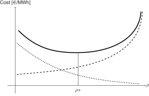
Figure 2.9 Total costs (solid line), interruption costs (dotted line) and reliability costs (dashed line) as a function of the reliability level  .
.
If sufficient data and a detailed understanding of the system is available, ![]() and
and ![]() could be differentiated in space (
could be differentiated in space (![]() ), by consumer group (
), by consumer group (![]() ) and in time (
) and in time (![]() ):
):

2.4.3 Minimizing the Sum of Reliability and Interruption Costs
The objective of reliability management is to determine and execute those actions that maximize total socio-economic welfare. However, under two simplifying assumptions, minimization of the sum of reliability and interruption costs is a good proxy for welfare maximization. The assumptions are that changes in the electricity market should (i) not change the behavior of electricity market actors, such as producers and consumers, and (ii) have little effect on other markets. These two assumptions are off course never fully met. For example, if electricity becomes more expensive, consumers will (i) buy slightly less electricity and (ii) have less budget left to buy other goods. The optimal reliability level is then the level at which the sum of reliability and interruption costs is minimized.
Figure 2.9 plots expected total costs (solid line) of the electricity market as a function of the reliability level ![]() . The dotted line represents expected interruption costs, decreasing with the reliability level, while the dashed line represents reliability costs, increasing with the reliability level. If the reliability level is too high, expected interruption costs are too low while reliability costs are too high. If the reliability level is too low, expected interruption costs are too high while reliability costs are too low.
. The dotted line represents expected interruption costs, decreasing with the reliability level, while the dashed line represents reliability costs, increasing with the reliability level. If the reliability level is too high, expected interruption costs are too low while reliability costs are too high. If the reliability level is too low, expected interruption costs are too high while reliability costs are too low.
The exact shape of the expected interruption costs and reliability costs function is difficult to assess. To determine if certain costly actions are increasing or decreasing total costs, one has to compare the marginal cost and benefits of all possible actions. That is, one has to trade off the cost of an action and the resultant decrease of expected interruption costs.
For example, assume that three possible actions are available:
- 1. increased maintenance spending,
- 2. an investment in a new transmission line,
- 3. decreasing the generation reserve margin.
Table 2.3 summarizes the reliability cost of these actions, expressed per hour, as well as their effect on expected energy not supplied (EENS). Assuming a VOLL of 5000 €/MWh, the change of expected interruption cost is also calculated. The example in this table shows that the reliability cost of both increased maintenance spending and a transmission line investment is higher than the benefit of decreased expected interruption cost. However, decreasing the generation reserve margin is cost-decreasing since the reliability cost decrease is higher than the EIC increase.
Table 2.3 Illustrative example of reliability cost and interruption cost of different network operator actions
| Action | Reliability | VOLL | ||
| cost |
||||
| Increased maintenance spending | 350 | −0.04 | 5000 | −200 |
| Transmission line investment | 800 | −0.1 | 5000 | −500 |
| Decreased generation reserve margin | −500 | 0.06 | 5000 | 300 |
Clearly, the parameters used in this example might not be certain in advance. For example, if the VOLL were 10 000 €/MWh instead of 5000 €/MWh – that is, the societal consequences of the expected interruptions are higher – increasing maintenance spending would decrease total costs. Likewise, if the effect of the transmission line investment on EENS were -0.2 MWh/hour instead of -0.1 MWh/hour, this investment action would also decrease total costs. However, this does not imply that each action that decreases the sum of reliability and interruption costs is an efficient action. One should first determine and execute those actions that have the highest ratio of benefits versus costs, up to the point where the ratio of benefits and cost equals one for the most efficient actions. That is, up to the point where the marginal benefit equals the marginal cost.
2.5 Conclusion
An adequate reliability level in the power system is crucial, as it is one of the most critical infrastructures for the economy and social wellbeing of a modern society. Security is an important aspect determining a power system's reliability level, next to the adequacy of the system. Due to evolutions in the systems resulting in increased uncertainties, the currently used reliability management strategies based on a deterministic N–1 reliability criterion are being challenged. More advanced methodologies might be required in order to handle uncertainties in different timeframes in an appropriate way and to obtain a balance between reliability cost and interruption cost. Such criteria not only need to manage uncertainty – they also need to take into account the changing requirements over different time horizons, from planning to real time operations.
References
- 1 Kirschen, D. (2002) Power system security. Power Engineering Journal, 16 (5), 241–248.
- 2 NERC Operating Committee and NERC Planning Committee (2007), Definition of “adequate level of reliability”, http://www.nerc.com/docs/pc/Definition-of-ALR-approved-at-Dec-07-OC-PC-mtgs.pdf.
- 3 International Electrotechnical Commission and others (2009). IEC/IEV 617-01-01. Electropedia: The world's online electrotechnical vocabulary, http://www.electropedia.org/.
- 4 Billinton, R. and Allan, R.N. (1984) Power system reliability in perspective. Electronics and Power, 30 (3), 231–236.
- 5 Knight, U.G. (2001) Power systems in emergencies: From contingency planning to crisis management, John Wiley & Sons, Ltd.
- 6 Allan, R. and Billinton, R. (2000) Probabilistic assessment of power systems. Proceedings of the IEEE, 88 (2), 140–162.
- 7 Hofmann, M., Kjølle, G., and Gjerde, O. (2012) Development of indicators to monitor vulnerabilities in power systems, in PSAM11/ESREL2012, Helsinki.
- 8 Kjølle, G., Gjerde, O., and Hofmann, M. (2013) Vulnerability and security in a changing power system. SINTEF Energy Research, Trondheim, p. 51.
- 9 ENTSO-E (2016) System operation guideline, Tech. Rep., ENTSO-E. URL http://networkcodes.entsoe.eu/operational-codes/operational-security/.
- 10 Task Force C4.601 CIGRE (2010) Review of the current status of tools/techniques for risk based and probabilistic planning in power systems.
- 11 Allan, R. and Billinton, R. (2000) Probabilistic assessment of power systems. Proceedings of the IEEE, 88 (2), 140–162.
- 12 Billinton, R. and Wenyuan, L. (1991) Hybrid approach for reliability evaluation of composite generation and transmission systems using Monte-Carlo simulation and enumeration technique. IEE Proceedings C-Generation, Transmission and Distribution, 138 (3), 233–241.
- 13 Meliopoulos, S., Taylor, D., Singh, C., Yang, F., Kang, S. W., and Stefopoulos, G. (2005), Comprehensive power system reliability assessment. PSERC Publication 05–13.
- 14 Niebur, D. and Fischl, R. (1997) Artificial intelligence techniques in power systems, chapter Artificial neural networks for static security assessment, pages 143–191. Number 22, IET.
- 15 Monticelli, A., Pereira, M.V.F., and Granville, S. (1987), Security-constrained optimal power flow with post-contingency corrective rescheduling. IEEE Transactions on Power Systems, 2 (1), 175–180.
- 16 ENTSOE (2009) Policy 3: Operational security, Tech. Rep., ENTSOE.
- 17 ENTSO-E subgroup: system protection and dynamics (2012) Special protection schemes, Tech. Rep., ENTSO-E.
- 18 Ejebe, G.C. and Wollenberg, B.F. (1979) Automatic contingency selection. IEEE Transactions on Power Apparatus and Systems, PAS-98 (1), 97–109.
- 19 Chen, Q. and McCalley, J.D. (2005) Identifying high risk N-k contingencies for online security assessment. IEEE Transactions on Power Systems, 20 (2), 823–834.
- 20 ENTSOE (2015) Policy 5: Emergency operations, Tech. Rep., ENTSOE.
- 21 ENTSOE (2010) Appendix policy 5: Emergency operations, Tech. Rep., ENTSOE.
- 22 ENTSOE (2010) Technical background and recommendations for defence plans in the continental europe synchronous area, Tech. Rep., ENTSOE.
- 23 S. De Boeck and D. Van Hertem (2013) Coordination of multiple HVDC links in power systems during alert and emergency situations, in PowerTech (POWERTECH), 2013 IEEE Grenoble, pp. 1–6.
- 24 Reppen, N.D. (2004) Increasing utilization of the transmission grid requires new reliability criteria and comprehensive reliability assessment, in Probabilistic Methods Applied to Power Systems, 2004 International Conference on, IEEE, pp. 933–938.
- 25 Billinton, R. and Allan, R. (1984) Power system reliability in perspective. Electronics and Power, 30 (3), 231–236.
- 26 Li, W. and Choudhury, P. (2008) Probabilistic planning of transmission systems: Why, how and an actual example, in Power and Energy Society General Meeting-Conversion and Delivery of Electrical Energy in the 21st Century, 2008 IEEE, IEEE, pp. 1–8.
- 27 Kirschen, D. and Jayaweera, D. (2007) Comparison of risk-based and deterministic security assessments. IET Generation, Transmission & Distribution, 1 (4), 527–533.
- 28 Allan, R., Billinton, R., Breipohl, A., and Grigg, C. (1999) Bibliography on the application of probability methods in power system reliability evaluation. IEEE Transactions on Power Systems, 14 (1), 51–57.
- 29 Heylen, E. and Van Hertem, D. (2014) Importance and difficulties of comparing reliability criteria and the assessment of reliability, in Young Researchers Symposium, Ghent, EESA.
- 30 CEER (2010) Guidelines of Good Practice on Estimation of Costs due to Electricity Interruptions and Voltage Disturbances, Tech. Rep. December.
- 31 NERC (2013) State of Reliability 2015, Tech. Rep. May.
- 32 Heylen, E., Labeeuw, W., Deconinck, G., and Van Hertem, D. (2016) Framework for evaluating and comparing performance of power system reliability criteria. IEEE Transactions on Power Systems, 31 (3), 5153–5162.
- 33 Reichl, J., Schmidthaler, M., and Schneider, F. (2013) The value of supply security: The costs of power outages to Austrian households, firms and the public sector. Energy Economics, 36, 256–261.
- 34 Pepermans, G. (2011) The value of continuous power supply for Flemish households. Energy Policy, 39 (12), 7853–7864.
- 35 de Nooij, M., Koopmans, C., and Bijvoet, C. (2007) The value of supply security. The costs of power interruptions: Economic input for damage reduction and investment in networks. Energy Economics, 29 (2), 277–295.