3.4. Doubly-Stochastic EM
This section presents an EM-based algorithm for problems that possesses partial data with multiple clusters. The algorithm is referred to as as a doubly-stochastic EM. To facilitate the derivation, adopt the following notations:
X = {xt ∊ RD; t = 1,..., T } is a sequence of partial-data.
Z = {zt ∊ C; t = 1, . . . , T} is the set of hidden-states.
C = {C(1), . . . ,C(J)}, where J is the number of hidden-states.
Г = {γ(1)), . . . , γ(K)} is the set of values that xt can attain, where K is the number of possible values for xt.
Also define two sets of indicator variables as:
![]()
![]()
Using these notations and those defined in Section 3.2, Q(θ|θn) can be written as
Equation 3.4.1

where

If θ defines a GMM—that is, θ = {π(j), μ(j), ![]() — then
— then

3.4.1. Singly-Stochastic Single-Cluster with Partial Data
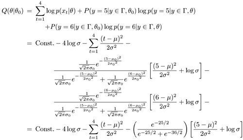
This section demonstrates how the general formulation in Eq. 3.4.1 can be applied to problems with a single cluster and partially observable data. Referring to Example 2 shown in Figure 3.3(b), let X = {x1, x2 x3, x4, y} = {1, 2, 3, 4, {5 or 6}} be the observed data, where y = {5 or 6} is the observation with missing information. The information is missing because the exact value of y is unknown. Also let z ∊ Г, where Г = {γ(1), γ(2)} = {5, 6}, be the missing information. Since there is one cluster only and x1 to x4 are certain, define θ ≡ {μ,σ2}, , set π(1) = 1.0 and write Eq. 3.4.1 as
Equation 3.4.2

Note that the discrete density p(y = γ((k)|y ∊ Г, θ) can be interpreted as the product of density p(y = γ(k)|y ∊ Г) and the functional value of p(y|θ) at y = γ(k) as shown in Figure 3.7.
Figure 3.7. The relationship between p(y|θ0), p(y|y ∊ Г), p(y|y ∊ Г, θ0), and P(y = γ(k) |y ∊ Г, θ0), where Г = {5, 6}.

Assume that at the start of the iterations, n = 0 and ![]() } = {0, 1}. Then, Eq. 3.4.2 becomes
} = {0, 1}. Then, Eq. 3.4.2 becomes

Equation 3.4.3
![]()
In the M-step, compute θ1 according to
![]()
The next iteration replaces θ0 in Eq. 3.4.3 with θ1 to compute Q(θ|θ1). The procedure continues until convergence. Table 3.4 shows the value of μ and σ2 in the course of EM iterations when their initial values are μ0 = 0 and ![]() . Figure 3.8 depicts the movement of the Gaussian density function specified by μ and σ2 during the EM iterations.
. Figure 3.8 depicts the movement of the Gaussian density function specified by μ and σ2 during the EM iterations.
| Iteration (n) | Q(θ|θn) | μ | σ2 |
|---|---|---|---|
| 0 | −∞ | 0.00 | 1.00 |
| 1 | -29.12 | 3.00 | 7.02 |
| 2 | -4.57 | 3.08 | 8.62 |
| 3 | -4.64 | 3.09 | 8.69 |
| 4 | -4.64 | 3.09 | 8.69 |
| 5 | -4.64 | 3.09 | 8.69 |
Figure 3.8. Movement of a Gaussian density function during the EM iterations. The density function is to fit the data containing a single cluster with partially observable data.

3.4.2. Doubly-Stochastic (Partial-Data and Hidden-State) Problem
Here, the single-dimension example shown in Figure 3.9 is used to illustrate the application of Eq. 3.4.1 to problems with partial-data and hidden-states. Review the following definitions:
X = {x1, x2,..., x6, y1, y2} is the available data with certain {x1,..., x6} and uncertain {y1, y2} observations.
 where zt and
  is the set of hidden-states.
 and
and  such that y1 ∊ Г1 and y2 ∊ Г2 are the values attainable by y1 and y2, respectively.
J = 2 and K = 2.
Figure 3.9. Single-dimension example illustrating the idea of hidden-states and partial-data.

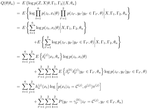
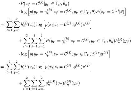
Using the preceding notations results in


Equation 3.4.4
![]()
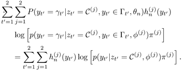
where ![]() is the posterior probability that yt' is equal to
is the posterior probability that yt' is equal to ![]() given that yt' is generated by cluster C(j). Note that when the values of y1 and y2 are certain (e.g., it is known that y1 ═┴ 5, and
given that yt' is generated by cluster C(j). Note that when the values of y1 and y2 are certain (e.g., it is known that y1 ═┴ 5, and ![]() and
and ![]() become so close that we can consider y2 = 9), then K = 1 and Г1 = {γ1} = {5} and Г2 = {γ2} = {9}. In such cases, the second term of Eq. 3.4.4 becomes
become so close that we can consider y2 = 9), then K = 1 and Г1 = {γ1} = {5} and Г2 = {γ2} = {9}. In such cases, the second term of Eq. 3.4.4 becomes
Equation 3.4.5

Replacing the second term of Eq. 3.4.4 by Eq. 3.4.5 and seting x7 = y1 and x8 = y2 results in

which is the Q-function of a GMM without partially unknown data with all observable data being certain.
