4.4. Linear SVMs: Fuzzy Separation
Sometimes the training data points are not clearly separable, and most often, they are best characterized as "fuzzily" separable. It is therefore convenient to introduce the notion of a fuzzy (or soft) decision region to cope with such situations. For the nonseparable cases, it is not possible to construct a linear hyperplane decision boundary without incurring classification errors. A fuzzy SVM is a model that allows a more relaxed separation, which in turn would facilitate a more robust decision.
For fuzzy SVM classifiers, it is no longer suitable to talk about the separation width. Instead, it is more appropriate to adopt a notion of fuzzy region or, more exactly, fuzzy separation region. Accordingly, the distance ![]() takes a new meaning as the width of fuzzy separation.
takes a new meaning as the width of fuzzy separation.
4.4.1. Why Fuzzy Separation?
This section extends discussion of the basic SVM to a fuzzy SVM. From the biometric authentication perspective, the fuzzy SVM serves a practical purpose because it can provide the user with a probabilistic recommendation as opposed to a black-and-white decision. This can be useful for two scenarios:
In some applications, there will be combined sensors (e.g., visual and audio) for high-security access control. The decisions made by an individual sensor would best be soft, so that they can be properly weighted when all information is fused to reach a final decision of the joint-sensor classifier.
Another scenario is that, even if only a single sensor is used, the information is processed by a hierarchical structure (see Chapter 6); then, information from different local experts or classes will have to be combined. It is often observed that final decisions made by combining local information expressed in terms of soft decisions tends to yield superior performance, when compared with final decisions based on hard local decisions.
If the data patterns are not separable by a linear hyperplane, a set of slack variables {ξ = ξ1,…, ξN} is introduced with ξi ≥ 0 such that Eq. 4.3.9 becomes
Equation 4.4.1
![]()
The slack variables
![]() allow some data to violate the constraints noted in Eq. 4.3.9, which defines the minimum safety margin required for training data in the clearly separable case. (Recall that the safety margin is
allow some data to violate the constraints noted in Eq. 4.3.9, which defines the minimum safety margin required for training data in the clearly separable case. (Recall that the safety margin is ![]() ) The slack variables measure the deviation of data points from the marginal hyperplane. Equivalently, they measure how severely the safety margin is violated. In other words, in the fuzzy SVM, the minimum safety margin is relaxed by the amount specified by {ξi}. (In the clearly separable case, no such violation is allowed.) In this sense, the slack variables also indicate the degree of fuzziness embedded in the fuzzy classifier.
) The slack variables measure the deviation of data points from the marginal hyperplane. Equivalently, they measure how severely the safety margin is violated. In other words, in the fuzzy SVM, the minimum safety margin is relaxed by the amount specified by {ξi}. (In the clearly separable case, no such violation is allowed.) In this sense, the slack variables also indicate the degree of fuzziness embedded in the fuzzy classifier.
4.4.2. Wolfe Dual Optimization
The greater ξi is the less confidence one can in the decision, thus consider Σi ξi to be the upperbound of the training error. The new objective function to be minimized becomes
Equation 4.4.2
![]()
where C is a user-defined penalty parameter to penalize any violation of the safety margin for all training data. (Recall that the safety margin is defined to be ![]() ) Note also that a larger C means a heavier penalty will be imposed for the same level of violation.
) Note also that a larger C means a heavier penalty will be imposed for the same level of violation.
The new Lagrangian is
Equation 4.4.3
![]()
where αi ≥ 0 and βi ≥ 0 are, respectively, the Lagrange multipliers to ensure that yi(xi w + b) ≥ 1 - ξi and that ξi > 0. With some mathematical manipulation (see Problem 4), the Wolfe dual is obtained:
Equation 4.4.4

subject to 0 ≤ αi ≤ C, i = 1,..., N, ![]() .
.
Similar to the basic SVM, the output weight vector is

and the bias term is found by
![]()
where yk = 1 and xk is a support vector that lies on the plane wT x + b = 1.
Margin of Fuzzy Separation
The distance ![]() represents the margin of fuzzy separation. The larger the margin, the fuzzier is the classification.
represents the margin of fuzzy separation. The larger the margin, the fuzzier is the classification.
Note that a smaller C leads to more SVs while a larger C leads to fewer SVs.
Also note that a smaller C leads to a wider width of fuzzy separation, while a larger C has a narrower fuzzy separation region.
Analytical Examples
Example 4.4: 5-point linearly nonseparable problem
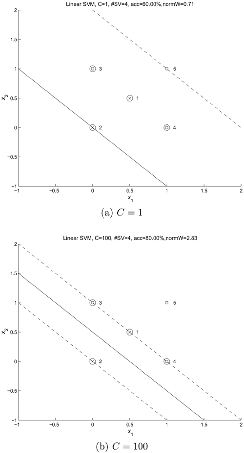
This example investigates the effect of varying C on the number of support vectors and the margin width in a linear SVM. Assume that the data points and their class labels are as follows:
The decision boundaries created by a linear SVM for this five-point linearly nonseparable problem for C - 1 and C - 100 are shown in Figure 4.3. Note that for small C, support vectors (Points 1, 3, and 4) fall between the margin because the cost of making a mistake is smaller for small C. On the other hand, when C is large, there is no SV that falls in the fuzzy region because the cost of making an error is higher for large C.
Figure 4.3. Five-point problem: (a) C = 1 and (b) C = 100. (See Example 4.4 for details.)
Example 4.5: Analytical solutions for a 4~point XOR problem
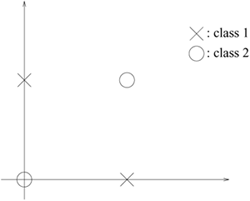
This example demonstrates how the Wolfe dual formulation can be applied to solve the classic XOR problem shown in Figure 4.4 using linear SVMs. Assume that the training data are defined as
Figure 4.4. The XOR problem. Clearly, the XOR problem is not linearly separable, but it can be separated by a nonlinear decision boundary.
Using the procedure described in Example 4.1, the following Lagrangian for a linear SVM is obtained:
Equation 4.4.5
Differentiating Eq. 4.4.5 with respect to A and αi, results in
Since x4 is not a support vector, the derivative of F(α, λ) with respect to α4 needs not be 0. Therefore, the fourth equation can be ignored, which results in
Therefore, the decision boundary will be identical to that of the three-point problem shown in Example 4.1 and Figure 4.2.
Readers' attention is drawn to the fact that while the analytical method can find a solution for this four-point XOR problem (because it is possible to manually discard the non-SV), the quadratic programming approach cannot find a decision boundary. In particular, the quadratic programming approach leads to the solution: αi = C∀ i, w = [0 0]T, and b = 0. Therefore, the decision boundary found by the quadratic programming approach reduces to a point in the input space.
4.4.3. Support Vectors in the Fuzzy Region
Because no slack variables were introduced in Section 4.3.2, there is only one kind of support vector in the basic SVM. More exactly, all support vectors lie on the margin of separation. However, with slack variables incorporated, more varieties of support vectors exist, which is elaborated on in this section.
The support vectors of the clearly separable and unclearly separable cases can be selected in almost the same manner. The only difference is that the Karush-Kuhn-Tucker conditions need to adopt a modified expression:
Equation 4.4.6
![]()
This equality states the necessary (and sometimes sufficient) conditions for which a set of variables will be optimal under the Wolfe optimization formulation. For example, the condition for a data point not being selected as a support vector is particularly simple, because
![]()
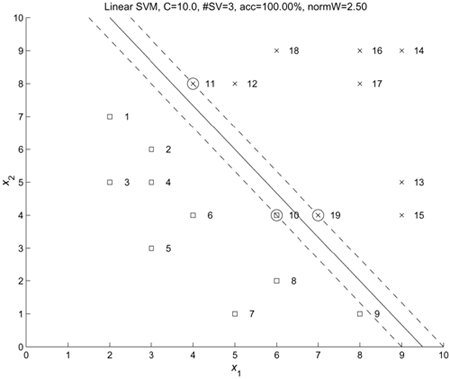
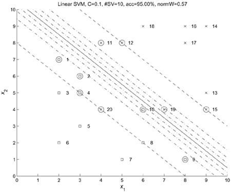
This relationship suggests that all non-SVs are generically outside the margin area (e.g., data points 4 and 15 in Figure 4.5(b)). A rare exception exists in a degenerate situation in which a data point satisfies
![]()
Then the data point will appear on the margin of the separation, even though it is theoretically possible that it is not selected to be a support vector. (See Problem 5.)
On the other hand, for a data point to be selected in the set of support vectors, it must precisely satisfy Eq. 4.4.1:
![]()
Now, examine this privileged set more closely. There are three types of SVs:
"On the margin" type: ξi = 0

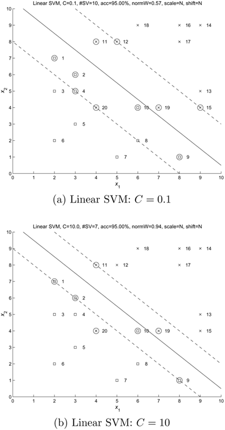
for example, Points 1, 2, 9, and 11 in Figure 4.5(b) belong to this type of support vector.
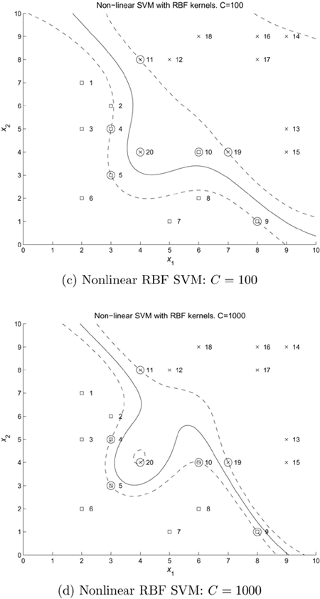
Figure 4.5. Decision boundaries (solid lines) and marginal boundaries (dashed lines) created by linear and nonlinear SVMs for 20-point data. (a) A linear SVM using C = 0.1, (b) a linear SVM with C = 10, (c) RBF SVM with C = 100, and (d) RBF SVM with C = 1000. (In both nonlinear cases (c) and (d), σ2 in Eq. 4.5.4 was set to 4.) The decision boundaries are almost the same for the two linear cases (a) and (b). The region between the two dashed lines are considered the "fuzzy region." Small C means a larger fuzzy region. This is consistent with the RBF kernel results. Note: The data set is obtained from Schwaighofer [149].
"Strictly inside the fuzzy region" type: 0 < ξi < 2

for example, Points 10 and 19 in Figure 4.5(b) belong to this type of support vector.
"Outliers" type: ξi ≥ 2

for example, Point 20 in Figure 4.5(b) belongs to this type of support vector. The existence of such outliers symbolizes an inconsistent message between training data and future generalization results. Some postprocessing treatment may be necessary to achieve a more agreeable accord. Practically, there are two ways to handle such outliers:
Further widen the fuzzy region so that the outliers can be relocated into the fuzzy region.
Weed the outliers out of the training set in the first place so as to preempt undue influence from the (erroneous) outliers.
Example 4.6: 20-point nonlinearly separable problem
In this example, a linear SVM is applied to classify 20 data points that are not linearly separable. Figure 4.5 depicts the decision boundary (solid line), the two lines (dashed) defining the margin, and the support vectors for C = 0.1 and C = 10. Observe that the margin is wider (i.e., decisions are more fuzzy) and that there are more support vectors when C is small.
Sparsity of Support Vectors
The SVM optimization methods are based on second-order optimality conditions (i.e., Karush-Kuhn-Tucker conditions), which reveal that the solution is sparse. This sparsity is one of the most important properties of SVMs because it makes SVM learning practical for large data sets.
4.4.4. Decision Boundary
Once the values of αi have been found from Eq. 4.4.4, the vector w can be determined just as before:

Once w is found, the value of threshold b can be computed exactly like the linearly separable case. This is made possible by exploiting the fact that
All the marginal support vectors can be readily identified because of the prior knowledge that 0 < αi < C if xi ∊ margin-set.
It is also known that ξi = 0 for all marginal support vectors: Xi ∊ margin-set.
Thus, the value of threshold b can be derived by solving the linear equation:
![]()
with w plugged in. Ultimately, the decision boundary can be derived as follows:
Equation 4.4.7

The decision boundary is dictated by the support vectors. This fact can be demonstrated by removing a support vector in the 20-point problem shown in Figure 4.5. Figure 4.6 illustrates the change in the decision boundary when Point 20 (a support vector in Figure 4.5) is removed from the training data set. Because the problem becomes a linearly separable one after the removal of this point, none of the support vectors falls in the fuzzy region.
Figure 4.6. The two-class problem in Figure 4.5 but without Point 20. Without this data point, the problem becomes a linearly separable one. Note the change in the decision boundary as compared to Figure 4.5(b).
4.4.5. Probabilistic Function for Decision Confidence
As shown in Figure 4.5, the region between the two dashed lines can be considered the fuzzy decision region. In this fuzzy region, assigning a probability (confidence) to the classification decision is highly recommended. There are two approaches to assigning probabilities:
Linearly proportional probability function. Two situations exist in this case: (1) If a data point is interior to the fuzzy region, assign 0.5(wTx + b + 1) as the probability of a data point belonging to the "positive-class" (i.e., yi = 1). Consequently, its "negative-class" probability is 1–0.5(wTx + b+1)=0.5(1 – wTx – b). Note that a pattern x is more likely to belong to the positive-class if f (x) > 0 and to the negative-class if f (x) < 0. (2) If a data point is exterior to the fuzzy region, it falls in the hard-decision region and its class probability will be either 1.0 or 0.0.
It is easy to show that the sigmoid value has a range of 0.0 to 1.0 for the entire vector space. Suppose the marginal support vectors are set for a confidence level of 1% or 99%, then
![]()
Figure 4.7 depicts the equal-probability contours of a linear SVM for the 20-point problem using σ = 0.22 and Eq. 4.4.8. Because the 20 data points shown in Figure 4.7 are not linearly separable, assigning a soft probability as the classification confidence for data in the fuzzy separation region is highly recommended.
Figure 4.7. Contour plot showing the probabilistic output of a linear SVM for the two-class problem shown in Figure 4.5. The margins (dashed lines) correspond to probabilities 0.0 or 1.0. The contour lines between the margins (dashed-dotted lines) represent probabilities 0.875, 0.750, and 0.625. Points on the decision boundary (solid line) have a probability of 0.5.
4.4.6. Invariance Properties of Linear SVMs
It can be shown that linear SVMs are invariant to both scaling and translation in the input domain. It is easier to establish invariance using the primal formulation (see Eq. 4.4.3). For proving scale invariance, w in the third term of Eq. 4.4.3 is scaled down by β. For proving translation invariance, b in the third term is replaced by b - wTt, where t is a translation vector. The proofs based on the Wolfe dual formulation, however, will be useful for investigating the invariance properties of nonlinear SVMs because there is no primal formulation for nonlinear SVMs.
Note that the invariance property of linear SVMs can also be proved by using the dual formulation Eq. 4.4.4. (See Problem 7.)


