
4.5. Nonlinear SVMs
It is well known that, by inserting a well-designed nonlinear hidden-layer between the input and output layers, a two-layer network can provide an adequate flexibility in the classification of fuzzily separable data. The original linearly nonseparable data points can be mapped to a new feature space, represented by hidden nodes such that the mapped patterns become linearly separable. This is illustrated in Figure 4.8.
Figure 4.8. Use of a kernel function to map nonlinearly separable data in the input space to a high-dimensional feature space, where the data become linearly separable.

If the hidden nodes can be expressed by a nonlinear function {ϕi(x)}, i = 1, . . . , K, a generalized decision function has the following form:

where
![]()
The nonlinear functions ![]() for the hidden nodes can be adaptively trained by various supervised learning algorithms. For this purpose, many different neural networks are discussed in Chapter 5. This section looks into one particular category of learning algorithms, including SVM, which exploits the vital fact that such a decision function retains a linear expression in terms of the parameters w and b. As a result, the optimization can be effectively carried out by simple linear techniques such as least-squares error, Fisher's discriminant, or SVMs.
for the hidden nodes can be adaptively trained by various supervised learning algorithms. For this purpose, many different neural networks are discussed in Chapter 5. This section looks into one particular category of learning algorithms, including SVM, which exploits the vital fact that such a decision function retains a linear expression in terms of the parameters w and b. As a result, the optimization can be effectively carried out by simple linear techniques such as least-squares error, Fisher's discriminant, or SVMs.
4.5.1. Two-Layer SVM Network Architectures
Recall that a linear decision function for the SVM derived previously has the following form:
To obtain a nonlinear decision boundary, thus enhancing the discrimination power, replace the inner-product (x · xi) with a nonlinear kernel K(x, xi) and obtain
Equation 4.5.1
Nonlinear Kernels
The decision function in Eq. 4.5.1 can be implemented by a two-layer architecture depicted in Figure 4.9, where it is shown that the original input space is mapped to a new feature space, manifested by the middle hidden-layer in the network.
Figure 4.9. The two-layer architecture of an SVM. Employing the nonlinearity inherent in the hidden-layer in a two-layer network, the original linearly nonseparable input space can be converted into a linearly separable feature space. (a) The two-layer architecture of an SVM with all possible kernels displayed; and (b) simplified SVM architecture: the only support vectors that need to be retained are shown as hidden nodes. Here, the support vectors are indexed by the set S = {s1, s2,…,sm}, where sm ∊ {1, 2,…, N}.

The basic idea behind the nonlinear SVM is to use a kernel function K(x, xi) to map the data x from the input space to the feature space on which the mapped data become linearly separable. The hidden units on the hidden-layer are represented by the kernel function adopted by the SVM. There are various forms of nonlinear kernels. Three typical examples are:
Equation 4.5.2
![]()
Equation 4.5.3
![]()
Equation 4.5.4
![]()
Therefore, the SVM can be reformulated to imitate several prominent two-layer neural models (see Chapter 5), including polynomial learning machines, radial basis function networks, and linear-basis multi-layer perceptrons (with a single sigmoidal hidden-layer).
Lagrangian Optimization in Dual Domain
Recall the Lagrangian in the linear case:

Suppose that the original training patterns X are not linearly separable; to enhance the discrimination ability, the linear inner product (xi · xj) is replaced by a nonlinear kernel function K(xi, xj). This leads to a generalized Lagrangian as follows:
Equation 4.5.5
Clearly Separable Case. The Lagrange multipliers {αi} are determined by maximizing L(a) subject to
 and α ≥ 0, i = 1,…,N.
Fuzzy Separable Case. The Lagrange multipliers {αi} are determined by maximizing L(α) subject to
 and 0 ≤ α ≤ C, i = 1,…, N, where C is a factor used to control the violation of the safety margin rule. Of course, a larger C means that a heavier penalty is imposed.[3]
[3] Although the primal problem formulation does not always exist for nonlinear SVM, the penalty parameter C still inherits the property that a larger (resp. smaller) C more heavily penalizes (resp. tolerate more leniently) the violation of the safety margin.
Once the values of the Lagrange multipliers {αi} are obtained, then the decision function can be derived as (cf. Eq. 4.3.18):
Equation 4.5.6

which matches the output of the network shown in Figure 4.9. In fact, the output of the network could be one of the following:
If a hard decision is preferred, the class of a pattern x can be determined based on the sign of f(x).
The network could also output the probability (or confidence) of a pattern x belonging to a class if a fuzzy classification is desired. Assuming that the sigmoidal probability function is adopted, the probability of x belonging to the positive-class is expressed as:
Equation 4.5.7

An example of probability contours based on this sigmoidal probability mapping function is shown in Figure 4.10. Note that a pattern x is more likely to belong to the positive-class (resp. negative-class) if f(x) > 0 (resp. if f(x) < 0).
Figure 4.10. Contour plots showing the probabilistic outputs of RBF SVMs in (a) a four-point XOR problem and (b) a noisy XOR problem. The margins (dashed lines) correspond to probabilities 0.0 or 1.0. The contour lines between the margins (dashed-dotted lines) represent probabilities 0.875, 0.750, and 0.625. Points on the decision boundary (solid line) have a probability of 0.5. The probability mapping function in Eq. 4.5.7 was used to map the SVM output f(x) to probability.

4.5.2. Hidden Nodes and Retrieving Speed
The two-layer architecture, as shown in Figure 4.9, can be adopted for classification in the retrieving or testing phase. The retrieving speed is proportional to the active hidden nodes required for decision making.
It is important to note that Figure 4.9(a) shows an upper-bound scenario that all training patterns are incorporated into the hidden-layer. In reality, the number of hidden nodes that actively participate in the output function is much smaller— compared to Figure 4.9(b). According to Eq. 4.5.6, only those hidden nodes corresponding to the support vectors (i.e., with αi ≠ 0) can influence the decision boundary. It is therefore sufficient to retain only the support vectors in the hidden-layer. Thus, the actual number of hidden nodes could be much smaller.
Therefore, network complexity is closely tied to the number of support vectors selected by the SVM learning process. The number of support vectors (or hidden units) is dictated by the so-called Karush-Kuhn-Tucker conditions discussed in Section 4.3.3. For example, if the RBF-kernel SVM is applied to the training data, the number of critical support vectors will be determined automatically, which will in turn dictate the required number of hidden units (i.e., the radial basis functions) in the hidden-layer. The number of SVs can easily get out of control, especially in the case of a large fuzzy region (i.e., small C). A disadvantage of using smaller C lies in the fact that it may select a large number of support vectors, thus slowing down processing speed in the retrieval phase.
Finite-Decomposition of Nonlinear Kernels
Fortunately, the number of hidden nodes can still be substantially reduced if the kernel can be expressed either exactly or by approximation as a finite decomposable representation. A nonlinear kernel is said to be finite-decomposable if and only if there exists an integer K such that:
In other words, the nonlinear kernel K(x, x') can be expressed as an inner product of two vectors induced in a finite-dimensional (i.e., K-dimensional) feature space. Note that not all kernels are finite decomposable. For example, while the second-order polynomial kernel is finite decomposable, the RBF kernels are not.
Note that finite-decomposable kernels are somewhat related to the eigenfunction decomposition of kernels, but they in their own right have different requirements.[4] (See Problem 18.) Note that the development of the SVM neither needs nor depends on the eigenfunction decomposition property, which appears to be unnecessarily restrictive to most practical applications.
[4] If the following orthogonality relationship holds true
then the decomposition also happens to qualify as an eigenfunction decomposition as formally introduced in the Mercer theorem [63, 241]. The eigenfunction decomposition property can be verified by this equality:
Two-Layer Architecture for a Finite-Decomposable Kernel
As in Eq. 4.5.5, the nonlinear kernel Lagrangian can be constructed without having to consider the existence of the feature space itself. However, if a finite-dimensional feature space exists and is easily identified, this fact can be harnessed effectively to simplify the network architecture and improve retrieval performance.
Example 4.7: Finite-decomposable polynomial kernel
The simplest example is the second-order polynomial kernel on a two-dimensional vector space. Suppose a two-dimensional vector x = [u v]T, then the kernel can be expressed as
where one denotes
Equation 4.5.8
In conclusion, for any two-dimensional classification problem, including the famous XOR, the feature dimension can be fixed to K = 6.
With a finite-decomposable kernel, the primal problem can also be formulated in a fashion similar to its linear counterpart. The primal problem is to minimize:
Equation 4.5.9
Consequently, the penalty parameter C inherits the property that a larger (resp. smaller) C penalizes more heavily (resp. tolerate more leniently) the violation of the safety margin.
The decision function can be derived as (cf. Eq. 4.3.18):
Equation 4.5.10
![]()
where
Equation 4.5.11
Thus the number of hidden nodes, in terms of φ(x)-function, can be fixed to K without having to consider how many SVs are selected. The fixed network architecture for such a special case is shown in Figure 4.11. It guarantees a constant size of hidden-layer, thereby saving implementation cost. In short, when the number of SVs is potentially large, finite-decomposable kernels, such as the second-order polynomial kernel, become a more attractive alternative because they result in a slimmer architecture and thus a faster retrieving speed.
Figure 4.11. For finite-decomposable kernels, the number of hidden nodes can be independent of the size of the training data and SVs. For example, the second-order polynomial kernel SVM can always be implemented with six hidden nodes, with one of the hidden node's output always being equal to 1.0.
4.5.3. Training Criteria and Running Time
The retrieving performance depends very much on the network structure itself. Taking a structural perspective, the SVM can be seen as a special case of multi-layer neural models and vice versa. From the training criteria perspective, however, there are fundamental differences [166]. It is important to have a thorough understanding of the issues related to the training criteria as well as the computational cost of the SVM.
SVM versus LSE Learning Criteria
As shown in Section 4.2, LSE and Fisher classifiers produce almost the same decision function. In fact, both the LSE and Fisher training criteria are tuned to be sensitive to all of the training data points. For comparison purposes, another prominent classifier is introduced here: RBF neural networks, which are usually trained by the back-propagation (BP) algorithm or a two-stage learning algorithm consisting of K-means, K-nearest neighbors, and least-squares methods (cf. Chapter 5). Just like the LSE classifier, the RBF neural networks are (1) based on a quadratic loss function (i.e., the mean-squared error), and (2) sensitive to the broad base of data distribution.
The key advantage to using a quadratic loss function lies in its elegant mathematical analysis and the existence of a closed-form solution—the latter is vital for lowering computational cost. However, such computational savings often come at the expense of compromised training accuracy.[5] Because a quadratic loss function is proportional to the squared errors, the data points further away from the decision boundary are given higher (and sometimes excessive) weighting to influence the decision boundary.
[5] Note that better training accuracy does not necessarily imply a better generalization performance, which in itself is an important measurement to be discussed in Section 4.5.4.
Via a geometrical criterion, the SVM effectively tackles this concern from two fronts:
The SVM criterion is sensitive only to marginal data points, instead of the overall data distribution, ruling out any possible influence from data points far away from the decision boundary.
The support vector learning algorithm minimizes a loss function that is linearly proportional to the degree of violation of a set of safety margins. Although such a criterion is not exactly the same as that of minimizing the probability of classification error, it is considered to be much less sensitive than the mean-squared error criterion.[6] In fact, the SVM can be considered an extension of the minimum absolute error criterion of minimax theory because it basically follows the principle of structural risk minimization.
[6] For neural networks, which aim to minimize classification error, see the discussion in Chapter 7.
Running Time in Training Phase
Unlike the popular BP algorithm, the support vector learning algorithm can operate only in batch mode. More critically, in terms of running time, SVMs appear to be slower than the back-propagation algorithm for a similar generalization performance [128].
The support vectors are usually a fraction of the total number of examples constituting the training sample. Such sparsity is desirable for the retrieving phase. However, the selection often must endure a long training process. The fundamental difficulty causing the slower processing time is that all training data points are potential candidates for the support vectors. Moreover, there is no control over the number of data points selected to be support vectors by the learning algorithm. In other words, an effective selection of support vectors remains a difficult and challenging issue, particularly for fuzzily separable patterns.
The selection of support vectors, which involves solving a quadratic programming problem, requires a long training time. Unfortunately, the memory size required for running the quadratic programming problem grows with the square of the size of the training data set. Such a lengthy computation time discourages or sometimes prohibits the SVMs from being directly applied to large-scale real-life problems.
Dealing with Large Data Sets
A novel decomposition scheme for cutting the running time of an SVM was proposed by Osuna et al. [267]. The scheme emphasizes the support vector multipliers that are around α = 0 and α = C. Reportedly, the proposed algorithm can attain reasonable optimization with satisfactory running time even for large-scale applications with up to 100,000 data points.
In addition, there are several ways to deal with large problem sets. For example, in the decomposition method [33, 267], a small, arbitrary subset of the training data is used to create an initial SVM, which is then tested by the remaining data. The distances between the test data and the margin are sorted in descending order, and the first N of these data together with the Ns support vectors already found are used to retrain the SVM. This process is repeated until all data have been used for training and all of them satisfy the Karush-Kuhn-Tucker conditions. In case the training data are obtained from a number of variable-length sequences (e.g., feature vectors extracted from speech utterances), it is possible to significantly reduce the amount of training data by computing the Fisher scores [160]. In this approach, the whole feature sequence of an utterance is replaced by a Fisher score, which is a vector in a high-dimensional space. SVMs are then trained on the vectors in this space.
Another possibility to reduce the amount of training data is to perform K-means or EM clustering on the large data set to find some representative training vectors prior to SVM training [364]. Two approaches worthy of closer investigation are suggested here:
One uses clustering to lower data resolution, resulting in more sparse training data; for example, see Section 4.5.5.
The second adopts some sort of prescreening scheme using, for example, Fisher scores as the screening criterion.
4.5.4. Generalization Performance of Nonlinear SVMs
Two kinds of training performances are often used to judge the success/failure of a learning algorithm.
Training Accuracy. For training accuracy, the test patterns are simply samples drawn from the original training patterns. Therefore, training accuracy is a good indication of the memorization capability of the trained model.
Generalization Accuracy. For generalization accuracy, in contrast, test patterns do not necessarily come from the original training patterns. Instead, they are drawn arbitrarily based on the same distribution function that originally generated the training patterns.
In short, the distinction between training and generalization accuracies lies in the test patterns adopted. Although high training accuracy guarantees good memorization capability, it does not necessarily yield good generalization accuracy. This suggests a fundamental tradeoff between training and generalization accuracies.
Impact of the C Parameter on Generalization Performance
Robustness of nonlinear SVMs is an important design consideration because it exerts a major influence on generalization performance. Just like the previous linear SVM case, the larger the value of C, the fewer critical SVs are selected to determine the final decision boundary. These support vectors are vital for the SVM to attain high training accuracy. Thus, the larger the value of C, the better the training accuracy.
However, from the generalization perspective, these selective SVs are not a good representation of the general statistical distribution of training data. A decision boundary with a focus on a small number of selected SVs is unlikely to deliver a good performance for test data drawn from a general distribution. So, when C is too large, it tends to lead to spurious or more curved decision boundaries. In other words, it suffers a side effect known as overtraining.
The robustness and generalization performance of nonlinear SVMs depends heavily on the degree of fuzziness of the support vector machine chosen. Because C is the penalty parameter to curb the training data's violation on the safety margin, thus it plays a key role in controlling the degree of fuzziness. A small, carefully adjusted C tends to relax the penalty on violating the safety margin, and thus enhances generalization performance, although sometimes at the expense of training accuracy.
Simulation Examples
To verify the preceding claims, experiments have been conducted in which RBF-and polynomial-kernel SVMs with different values of C were used for solving the noisy XOR problem. As shown in Figures 4.12(a) through 4.12(d), SVMs with small values of C yield smoother (and more desirable) boundaries as compared to those with large values of C. However, this phenomenon is not obvious in the polynomial-kernel SVMs, as shown in Figures 4.13(a) through (d). In other words, the decision boundaries created by polynomial-kernel SVMs seem to be less sensitive with respect to the change in C. This property can be considered an advantage of the polynomial kernels.
Figure 4.12. Experimental results of RBF-kernel SVMs on the noisy XOR problem with various values of C. In all cases, the width parameter a of the RBF kernel is set to 0.707.


Figure 4.13. Results of second-order polynomial-kernel SVMs on the noisy XOR problem with different values of C.
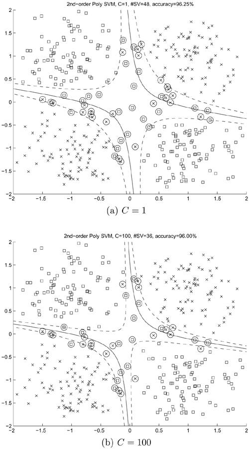
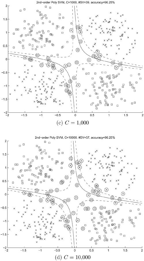
Recall that, in linear SVMs, a larger C delivers a narrower fuzzy separation region. In the nonlinear experiments, it has been observed that a larger C does make the fuzzy separation region a bit narrower. However, it can be observed that a larger C does cause the decision boundary (and marginal boundaries) to become more curved. Conversely, a smaller C usually results in a less curved decision boundary, and thus a more robust classifier. Therefore, choosing smaller C's for the purpose of yielding a more robust classifier and a more predictable generalization performance is recommended.
4.5.5. Effects of Scaling and Shifting
Shift Invariance Properties of Nonlinear SVMs
Shift invariance means that if training data are shifted by a translation vector t
![]()
then the decision boundary will also be shifted by the same amount and the shape of the boundary will remain unchanged.
Recall from Section 4.4.6 that linear SVMs are shift invariant. On the other hand, it can be shown that the polynomial SVM is not shift invariant. Unlike its RBF counterpart, the polynomial kernel does not warrant a natural formulation to cope with the change in coordinates. Therefore, an optimal selection of coordinate systems can become critical for the polynomial kernel.
Example 4.8: Effect of coordinate translation on the XOR problem
For an analytical example, adopt a second-order polynomial kernel for the design of an SVM for the XOR problem. It is well known that a polynomial kernel function K(x, xi) may be expressed in terms of monomials of various orders. More precisely, denote x = [u v]T , then
A. The Original XOR Problem
As shown in Figure 4.14(a), there are two data points, (0, 0) and (1, 1), for one class and two points for the other, (1, 0) and (0, 1). Based on the vectors xi and class labels yi defined in Example 4.5, the Lagrangian function of interest is now:
subject to αi ≥ 0 and
Optimizing L(α) with respect to the Lagrange multipliers yields the following set of simultaneous equations:
Then the optimal Lagrange multipliers can be derived as α1 = 10/3, α2 = 8/3, α3 = 8/3, and α4 = 2. (The optimum value of L(α) is 18.) Thus, all of the training vectors are selected as SVs. The threshold is derived to be b = -1. Recall that
From Eq. 4.5.11, the optimum weight vector is found to be
which in turn leads to the following optimal decision boundary:
This decision boundary is illustrated in Figure 4.14(a), which is somewhat less desirable than that in Figure 4.14(b).
Figure 4.14. Effect of the translation of training data on polynomial SVMs based on the XOR problem: (a) Without shift and (b) training data are shifted (xi ← xi – [0.5 0.5]T) so that they are symmetric about the origin.
B. Coordinate-Shifted XOR Problem
As shown in Figure 4.14(b), there are two data points (–0.5, –0.5) and (0.5, 0.5) for one class and two points for the other, (–0.5, 0.5) and (0.5, –0.5). Now the Lagrangian becomes:
subject to αi ≥ 0 and
Solving the following simultaneous saddle-point equations:
results in α1 = 2, α2 = 2, α3 = 2, α4 = 2, and b = 0. From Eq. 4.5.11, the optimum weight vector is
This leads to a simple decision function:
which can be easily verified to satisfy the shifted XOR classification problem. As shown in Figures 4.14(a) and 4.14 (b), the two decision boundaries are very different: one for the original XOR and the other for the shifted XOR. The contention is that the latter decision boundary is better than the former because the latter has a centered data distribution, which seems to be a plus for the performance of polynomial-kernel SVM.


Example 4.9: Effect of shifting or coordinate translation on polynomial SVMs
Figures 4.15(a) and 4.15(b) illustrate the effect of shifting the training data on polynomial-kernel SVMs in the noisy XOR problem. Evidently, polynomial SVMs are not invariant to coordinate translation.
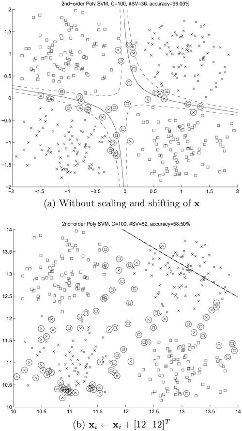
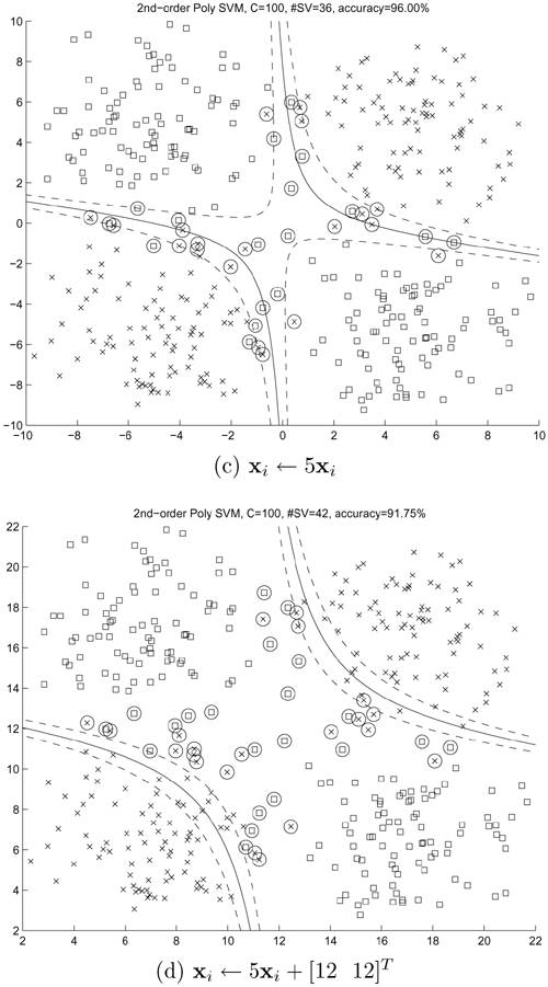
Figure 4.15. The effect of scaling and translation of training data on polynomial SVMs. The figures show the decision boundary and SVs for (a) training data xi without scaling and shifting, (b) training data shifted by [12 12]T (i.e., xi • xi + [12 12]T), (c) training data scaled by a factor of 5 (i.e., xi • 5xi), and (d) training data scaled by a factor of 5 and shifted by [12 12]T (i.e., xi • 5xi + [12 12]T). Note that for (c) and (d), the kernel function is also scaled: K(x, xi) = (1 + x · x/25)2. It can be seen that polynomial SVMs are invariant to scaling after proper adjustment on the kernel function; however, they are not invariant to translation of the training data. Note: Because of the translation in (b) and (d), the shape of the decision boundaries may be different in different simulation runs—for some runs, the decision boundaries are outside of the visible range.
Scale Invariance Properties of Nonlinear SVMs
Experiments have been conducted on RBF-kernel and polynomial-kernel SVMs on the noisy XOR problem and the results are shown in Figures 4.12(a) through 4.12(d) and Figures 4.13(a) through 4.13(d).
For all proposed kernel functions, the degree of nonlinearity depends on the parameter σ. The smaller σ, the more nonlinear the kernels become. Moreover, the more nonlinear the kernels, the better the training performance. This does not necessarily mean better generalization performance, however. For polynomial SVMs, the degree of the polynomial also plays an important role in controlling nonlinearity: the larger the degree, the more nonlinear the SVMs become.
Example 4.10: Effect of scaling on polynomial SVMs
Figures 4.15(a) and 4.15(c) illustrate the effect of scaling on polynomial SVMs in the noisy-XOR problem. Evidently, polynomial SVMs are invariant to scaling. Readers, however, should bear in mind that the scale invariance property of polynomial SVMs requires proper selection of the normalization parameter a. If this parameter is not proportionally scaled by the same amount as the training data, the decision boundary will not be proportionally scaled and the Lagrange multipliers corresponding to the scaled data will also be different from those of the unsealed data.
If necessary, the scale invariance of SVM can be enforced for RBF kernels as well as polynomial kernels. Suppose that the data are now scaled by β:
![]()
To enforce the scale invariance of SVMs, the following adjustment needs to be made:
![]()
It can be shown that the decision boundary will also be proportionally scaled by the same constant β.
Since the nonlinear version is formulated only in its dual domain (i.e., its formal primal problem is not well defined), the simple proof used in Section 4.4.6 cannot be applied. Here an alternative proof in the dual domain is provided. Assume the data are scaled by a constant factor β (i.e., x ← βx). Denote the scaled training data as ![]() (such that
(such that ![]() = βx) and the Lagrange multipliers corresponding to the scaled data as
= βx) and the Lagrange multipliers corresponding to the scaled data as ![]() . The Lagrangian for the scaled data is then
. The Lagrangian for the scaled data is then
Equation 4.5.12
where the following has been defined:
Equation 4.5.13
![]()
Because Eq. 4.5.12 has the same form as L(α), the Lagrange multipliers for the scaled SVM will not change (i.e., ![]() = αi ∀i). Note also that the bias b remains unchanged because
= αi ∀i). Note also that the bias b remains unchanged because

Since one has K1 (x',
![]() ) = K(x, xi) and
) = K(x, xi) and ![]() = αi ∀i, it is obvious that
= αi ∀i, it is obvious that
Therefore, the decision boundary is proportionally scaled.
Theoretically, it is also possible to use an alternative kernel function
Equation 4.5.14
![]()
to handle the scaling problem. It can be shown that the Lagrange multipliers for the scaled SVM become αi/β4 and the corresponding Lagrangian is L(α)/β4. (See Problem 8.) However, Eq. 4.5.14 should be used with caution because its range is significantly larger than that of Eq. 4.5.13, which may cause numerical difficulty in the quadratic programming optimizer [364].
It is obvious that polynomial SVMs are not translation invariant, because

where x' = x + t, and t is a translation vector.
The scale invariance and translation invariance properties of RBF SVMs can be proved in a similar way and are left to be done in an exercise.
Combine EM and RBF-SVM
The RBF kernel, ![]() , can benefit from an optimal selection
, can benefit from an optimal selection
of the parameter σ.[7] Therefore, the following hybrid supervised and unsupervised learning strategy, called EM-SVM, can be proposed.
[7] Proper adjustment on the scaling parameter σ is also required to improve the results of polynomial SVMs. In addition, since SVM is not translation invariant, the performance of polynomial SVMs could be further improved by using "data-centralized" coordinates.
In the unsupervised learning phase, the clustering methods (e.g., K-means or EM) are instrumental in revealing the intraclass subcluster structure. The K-means or EM techniques can be adopted to effectively derive the means and variances of intraclass subclusters (cf. Chapter 3).
In the supervised learning phase, two options can be considered:
If the size of original data points is manageable, select an appropriate σ according to the estimated variances. Since scaling can have a significant affect, an RBF-SVM can potentially deliver better performance with properly chosen variances.
More aggressively, if the original data points are too numerous, then it is imperative to force a reduction in training data: All data points in that subcluster will be represented by a single data point located at the cluster centroid. With such drastically reduced training data, running time of the EM-SVM learning can be substantially expedited.
Furthermore, the effectiveness of the training process is accomplished in two ways:
As discussed previously, fuzziness is achieved by insisting on smooth boundaries, which can be done by incorporating a restraining penalty factor C into the SVM.
Fuzziness is also achieved by controlling the resolution in the data space in terms of the RBF's radius: To avoid sharp and spurious boundaries in local regions, it helps if data are viewed with a somewhat coarser resolution, very much like passing through a smoothing low-pass filter.
Thus, the generalization performance of RBF-SVM is in a sense doubly assured.