
CHAPTER 17
Digital Signal Processing
In many ways, digital signal processing (DSP) returns us to the elemental beginning of our discussion of digital audio. Although conversion, error correction, data reduction, and other concerns can be critical to a digitization system, it is the software-driven signal processing of digital audio data that is germane to the venture. Without the ability to manipulate the numbers that comprise digital audio data, its digitization would not be useful for many applications. Moreover, a discussion of digital signal processing returns us to the roots of digital audio in that the technology is based on the same elemental mathematics that first occupied us. On the other hand, digital signal processing is a science far removed from simple logic circuits, with sophisticated algorithms required to achieve its aim of efficient signal manipulation. Moreover, digital signal processing may demand very specialized hardware devices for successful operation.
Fundamentals of Digital Signal Processing
Digital signal processing is used to generate, analyze, alter, or otherwise manipulate signals in the digital domain. It is based on sampling and quantization, the same principles that make digital recording possible. However, instead of providing a storage or transmission means, it is a processing method. DSP is similar to the technology used in computers and microprocessor systems. However, whereas a regular computer processes data, a DSP system processes signals. In particular, a digital audio signal is a time-based sequence in which the ordering of values is critical. A digital audio signal only makes sense, and can be processed properly, if the sequence is properly preserved. DSP is thus a special application of general data processing. Simply stated, DSP uses a mathematical formula or algorithm to change the numerical values in a bitstream signal.
A signal can be any natural or artificial phenomenon that varies as a function of an independent variable. For example, when the variable is time, then changes in barometric pressure, temperature, oil pressure, current, or voltage are all signals that can be recorded, transmitted, or manipulated either directly or indirectly. Their representation can be either analog or digital in nature, and both offer advantages and disadvantages.
Digital processing of acquired waveforms offers several advantages over processing of continuous-time signals. Fundamentally, the use of unambiguous discrete samples promotes: the use of components with lower tolerances; predetermined accuracy; identically reproducible circuits; a theoretically unlimited number of successive operations on a sample; and reduced sensitivity to external effects such as noise, temperature, and aging. The programmable nature of discrete-time signals permits changes in function without changes in hardware. Digital integrated circuits are small, highly reliable, low in cost, and capable of complex processing. Some operations implemented with digital processing are difficult or impossible with analog means. Examples include filters with linear phase, long-term uncorrupted memory, adaptive systems, image processing, error correction, data reduction, data compression, and signal transformations. The latter includes time domain to frequency-domain transformation with the discrete Fourier transform (DFT) and special mathematical processing such as the fast Fourier transform (FFT).
On the other hand, DSP has disadvantages. For example, the technology always requires power; there is no passive form of DSP circuitry. DSP cannot presently be used for very high frequency signals. Digital signal representation of a signal may require a larger bandwidth than the corresponding analog signal. DSP technology is expensive to develop. Circuits capable of performing fast computation are required. Finally, when used for analog applications, analog-to-digital (A/D) and digital-to-analog (D/A) conversion are required. In addition, the processing of very weak signals such as antenna signals or very strong signals such as those driving a loudspeaker, presents difficulties; digital signal processing thus requires appropriate amplification treatment of the signal.
DSP Applications
In the 1960s, signal processing relied on analog methods; electronic and mechanical devices processed signals in the continuous-time domain. Digital computers generally lacked the computational capabilities needed for digital signal processing. In 1965, the invention of the fast Fourier transform to implement the discrete Fourier transform, and the advent of more powerful computers, inspired the development of theoretical discrete-time mathematics, and modern DSP.
Some of the earliest uses of digital signal processing included soil analysis in oil and gas exploration, and radio and radar astronomy, using mainframe computers. With the advent of specialized hardware, extensive applications in telecommunications were implemented including modems, data transfer between computers, and vocoders and transmultiplexers in telephony. Medical science uses digital signal processing in processing of X-ray and NMR (nuclear magnetic resonance) images. Image processing is used to enhance photographs received from orbiting satellites and deep-space vehicles. Television studios use digital techniques to manipulate video signals. The movie industry relies on computer-generated graphics and 3D image processing. Analytical instruments use digital signal transforms such as FFT for spectral and other analysis. The chemical industry uses digital signal processing for industrial process control. Digital signal processing has revolutionized professional audio in effects processing, interfacing, user control, and computer control. The consumer sees many applications of digital signal processing in the guise of personal computers, cell phones, gaming consoles, MP3 players, DVD and Blu-ray players, digital radio receivers, HDTV receivers and displays, and many other devices.
DSP presents rich possibilities for audio applications. Error correction, multiplexing, sample rate conversion, speech and music analysis and synthesis, data reduction and data compression, filtering, adaptive equalization, dynamic compression and expansion, reverberation, ambience processing, time alignment, acoustical noise cancellation, mixing and editing, encryption and watermarking, and acoustical analysis can all be performed with digital signal processing.
Discrete Systems
Digital audio signal processing is concerned with the manipulation of audio samples. Because those samples are represented as numbers, digital audio signal processing is thus a science of calculation. Hence, a fundamental understanding of audio DSP must begin with its mathematical essence.
When the independent variable, such as time, is continuously variable, the signal is defined at every real value of time (t). The signal is thus a continuous time-based signal. For example, atmospheric temperature changes continuously throughout the day. When the signal is only defined at discrete values of time (nT), the signal is a discrete time signal. A record of temperature readings throughout the day is a discrete time signal. As we observed in Chap. 2, using the sampling theorem, any bandlimited continuous time function can be represented without theoretical loss as a discrete time signal. Although general discrete time signals and digital signals both consist of samples, a general discrete time signal can take any real value but a digital signal can only take a finite number of values. In digital audio, this requires an approximation using quantization.
Linearity and Time-Invariance
A discrete system is any system that accepts one or more discrete input signals x(n) and produces one or more discrete output signals y(n) in accordance with a set of operating rules. The input and output discrete time signals are represented by a sequence of numbers. If an analog signal x(t) is sampled every T seconds, the discrete time signal is x(nT), where n is an integer. Time can be normalized so that the signal is written as x(n).
Two important criteria for discrete systems are linearity and time-invariance. A linear system exhibits the property of superposition: the response of a linear system to a sum of signals is the sum of the responses to each individual input. That is, the input x1(n) + x2(n) yields the output y1(n) + y2(n). A linear system exhibits the property of homogeneity: the amplitude of the output of a linear system is proportional to that of the input. That is, an input ax(n) yields the output ay(n). Combining these properties, a linear discrete system with the input signal ax1(n) + bx2(n) produces an output signal ay1(n) + by2(n) where a and b are constants. The input signals are treated independently, the output amplitude is proportional to that of the input, and no new signal components are introduced. As described in the following paragraphs, all z-transforms and Fourier transforms are linear.
A discrete time system is time-invariant if the input signal x(n - k) produces an output signal y(n - k) where k is an integer. In other words, a linear time-invariant discrete (LTD) system behaves the same way at all times; for example, an input delayed by k samples generates an output delayed by k samples.
A discrete system is causal if at any instant the output signal corresponding to any input signal is independent of the values of the input signal after that instant. In other words, there are no output values before there has been an input signal. The output does not depend on future inputs. As some theorists put it, a causal system doesn’t laugh until after it has been tickled.
Impulse Response and Convolution
The impulse response is an important concept in many areas, including digital signal processing. The impulse response h(n) gives a full description of a linear time-invariant discrete system in the time domain. An LTD system, like any discrete system, converts an input signal into an output signal, as shown in Fig. 17.1A. However, an LTD system has a special property such that when an impulse (a delta function) is applied to an LTD system, the output is the system’s impulse response, as shown in Fig. 17.1B. The impulse response describes the system in the time domain, and can be used to reveal the frequency response of the system in the frequency domain. Practically speaking, most digital filters are LTD systems, and yield this property. A system is stable if any input signal of finite amplitude produces an output signal of finite amplitude. In other words, the sum of the absolute value of every input and the impulse response must yield a finite number. Useful discrete systems are stable.
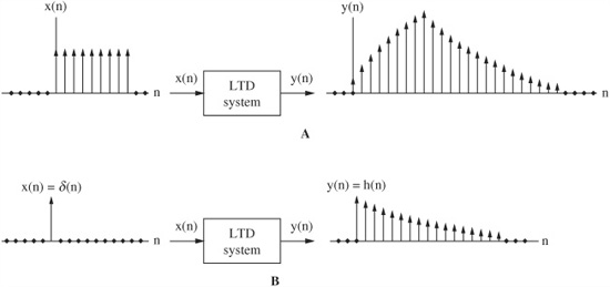
FIGURE 17.1 Two properties of linear time-invariant discrete (LTD) systems. A. LTD systems produce an output signal based on the input. B. LTD systems can be characterized by their impulse response, the output from a single pulse input.
Furthermore, the sampled impulse response can be used to filter a signal. Audio samples themselves are impulses, represented as numbers. The signal could be filtered, for example, by using the samples as scaling values; all of the values of a filter’s impulse response are multiplied by each signal value. This yields a series of filter impulse responses scaled to each signal sample. To obtain the result, each scaled filter impulse response is substituted for its multiplying signal sample. The filter response can extend over many samples; thus, several scaled values might overlap. When these are added together, the series of sums forms the new filtered signal values.
This is the process of convolution. The output of a linear system is the convolution of the input and the system’s impulse response. Convolution is a time-domain process that is equivalent to the multiplication of the frequency responses of two networks. Convolution in the time domain is equivalent to multiplication in the frequency domain. Furthermore, the duality exists such that multiplication in the time domain is equivalent to convolution in the frequency domain.
Fundamentally, in convolution, samples (representing the signal at different sample times) are multiplied by weighting factors. These products are continually summed together to produce an output. A finite impulse response (FIR) oversampling filter (as described in Chap. 4) provides a good example. A series of samples are multiplied by the coefficients that represent the impulse response of the filter, and these products are summed. The input time function has been convolved with the filter’s impulse in the time domain. For example, the frequency response of an ideal lowpass filter can be achieved by using coefficients representing a time-domain sin(x)/x impulse response. The convolution of the input signal with coefficients results in a filtered output signal.
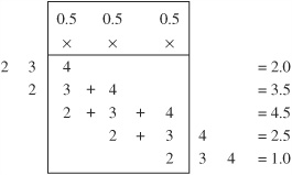
FIGURE 17.2 Convolution can be performed by folding, shifting, multiplying, and adding number sequences to generate an ordered weighted product.
Recapitulating, the response of a linear and time-invariant system (such as a digital filter) over all time to an impulse is the system’s impulse response; its response to an amplitude scaled input sample is a scaled impulse response; its response to a delayed impulse is a delayed impulse response. The input samples are composed of a sequence of impulses of varying amplitude, each with a unique delay. Each input sample results in a scaled, time-delayed impulse response. By convolution, the system’s output at any sample time is the sum of the partial impulse responses produced by the scaled and shifted inputs for that instant in time.
Because convolution is not an intuitive phenomenon, some examples might be useful. Mathematically, convolution expresses the amount of overlap of one function as it is shifted over another function. Suppose that we want to convolve the number sequence 0.5,0.5,0.5 (representing an audio signal) with 4,3,2 (representing an impulse response). We reverse the order of the second sequence to 2,3,4 and shift the sequence through the first sequence, multiplying common pairs of numbers and adding the totals, as shown in Fig. 17.2. The resulting values are the convolution sum and define the output signal at sample times.
To illustrate this using discrete signals, consider a network that produces an output h(n) when a single waveform sample is input (refer to Fig. 17.1B). The output h(n) defines the network; from this impulse response we can find the network’s response to any input. The network’s complete response to the waveform can be found by adding its response to all of the individual sample responses. The response to the first input sample is scaled by the amplitude of the sample and is output time-invariantly with it. Similarly, the inputs that follow produce outputs that are scaled and delayed by the delay of the input. The sum of the individual responses is the full response to the input waveform:
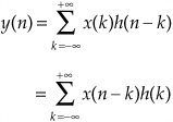
This is convolution, mathematically expressed as:
y(n) = x(n) * h(n) = h(n) * x(n)
where * denotes the convolution sum.
The output signal is the convolution of the input signal with the system’s impulse response. A convolution sum can be graphically evaluated by a process of folding, translating, multiplying, and shifting. The signal x(n) is the input to a linear shift invariant system characterized by the impulse response h(n), as shown in Fig. 17.3A. We can convolve x(n) with h(n) to find the output signal y(n). Using convolution graphically, we first fold h(n) to time-reverse it as shown in Fig. 17.3B. Folding is necessary to yield the correct time-domain response as we move the impulse response from left to right through the input signal. Also, h(n) is translated to the right, to a starting time. To view convolution in action, Fig. 17.3C shows h(n) shifting to the right, through x(n), one sample at a time. The values of samples coincident in time are multiplied, and overlapping time values are summed to determine the instantaneous output value. The entire sequence is obtained by moving the reversed impulse response until it has passed through the duration of the samples of interest, be it finite or infinite in length.
More generally, when two waveforms are multiplied together, their spectra are convolved, and if two spectra are multiplied, their determining waveforms are multiplied. The response to any input waveform can be determined from the impulse response of the network, and its response to any part of the input waveform. As noted, the convolution of two signals in the time domain corresponds to multiplication of their Fourier transforms in the frequency domain (as well as the dual correspondence). The bottom line is that any output signal can be considered to be a sum of impulses.
Complex Numbers
Analog and digital networks share a common mathematical basis. Fundamentally, whether the discussion is one of resistors, capacitors, and inductors, or scaling, delay, and addition (all linear, time-invariant elements), processors can be understood through complex numbers. A complex number z is any number that can be written in the form z = x + jy where x and y are real numbers, and where x is the real part, and jy is the imaginary part of the complex number. An imaginary number is any real number multiplied by j, where j is the square root of -1. There is no number that when multiplied by itself gives a negative number, but mathematicians cleverly invented the concept of an imaginary number. (Mathematicians refer to it as i, but engineers use j, because i denotes current.) The form x + jy is the rectangular form of a complex number, and represents the two-dimensional aspects of numbers. For example, the real part can denote distance, and the imaginary part can denote direction. A vector can be constructed, showing the indicated location.
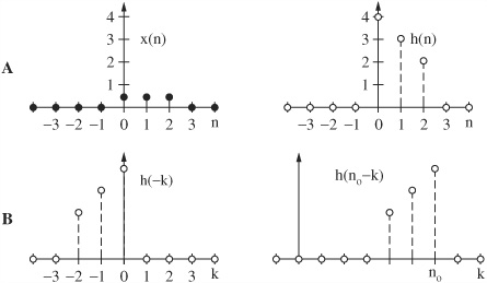
FIGURE 17.3 A graphical representation of convolution, showing signal x(n) convolved with h(n). A. An input signal x(n) and the impulse response h(n) of a linear time invariant system. B. The impulse response is folded and translated.
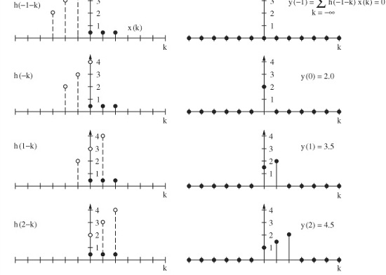
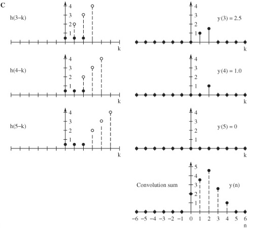
FIGURE 17.3 C. The convolution sum yields the output signal y(n).
A waveform can be described by a complex number. This is often expressed in polar form, with two parameters: r andϑ. The form rej also can be used. If a dot is placed on a circle and rotated, perhaps representing a waveform changing over time, the dot’s location can be expressed by a complex number. A location of 45° would be expressed as 0.707 + 0.707j. A location of 90° would be 0 + 1j, 135° would be -0.707 + 0.707j, and 180° would be -1 + 0j. The size of the circle could be used to indicate the magnitude of the number.
The j operator can be used to convert between imaginary and real numbers. A real number multiplied by an imaginary number becomes complex, and an imaginary number multiplied by an imaginary number becomes real. Multiplication by a complex number is analogous to phase-shifting; for example, multiplication by j represents a 90° phase shift, and multiplication by 0.707 + 0.707j represents a 45° phase shift. In the digital domain, phase shift is performed by time delay. A digital network composed of delays can be analyzed by changing each delay to a phase shift. For example, a delay of 10° corresponds to the complex number 0.984 - 0.174j. If the input signal is multiplied by this complex number, the output result would be a signal of the same magnitude, but delayed by 10°.
Mathematical Transforms
Signal processing, either analog or digital, can be considered in either of two domains. Together, they offer two perspectives on a unified theory. For analog signals, the domains are time and frequency. For sampled signals, they are discrete time and discrete frequency. A transform is a mathematical tool used to move between the time and frequency domains. Continuous transforms are used with signals continuous in time and frequency; series transforms are applied to continuous time and discrete frequency signals; and discrete transforms are applied to discrete time and frequency signals.
The analog relationships between a continuous signal, its Fourier transform, and Laplace transform are shown in Fig. 17.4A. The discrete-time relationships between a discrete signal, its discrete Fourier transform, and z-transform are shown in Fig. 17.4B. The Laplace transform is used to analyze continuous time and frequency signals. It maps a time-domain function x(t) into a frequency domain, complex frequency function X(s). The Laplace transform takes the form:
![]()
The inverse Laplace transform performs the reverse mapping. Laplace transforms are useful for analog design.
The Fourier transform is a special kind of Laplace transform. It maps a time-domain function x(t) into a frequency-domain function X(j), where X(j) describes the spectrum (frequency response) of the signal x(t). The Fourier transform takes the form:
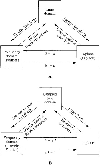
FIGURE 17.4 Transforms are used to mathematically convert a signal from one domain to another. A. Analog signals can be expressed in the time, frequency and s-plane domains. B. Discrete signals can be expressed in the sampled-time, frequency, and z-plane domains.
![]()
This equation (and the inverse Fourier transform), are identical to the Laplace transforms when s = j; the Laplace transform equals the Fourier transform when the real part of s is zero. The Fourier series is a special case of the Fourier transform and results when a signal contains only discrete frequencies, and the signal is periodic in the time domain.
Figure 17.5 shows how transforms are used. Specifically, two methods can be used to compute an output signal: convolution in the time domain, and multiplication in the frequency domain. Although convolution is conceptually concise, in practice, the second method using transforms and multiplication in the frequency domain is usually preferable. Transforms also are invaluable in analyzing a signal, to determine its spectral characteristics. In either case, the effect of filtering a discrete signal can be predictably known.
The Fourier transform for discrete signals generates a continuous spectrum but is difficult to compute. Thus, a sampled spectrum for discrete time signals of finite duration is implemented as the discrete Fourier transform (DFT). Just as the Fourier transform generates the spectrum of a continuous signal, the DFT generates the spectrum of a discrete signal, expressed as a set of harmonically related sinusoids with unique amplitude and phase. The DFT takes samples of a waveform and operates on them as if they were an infinitely long waveform composed of sinusoids, harmonically related to a fundamental frequency corresponding to the original sample period. An inverse DFT can recover the original sampled signal. The DFT can also be viewed as sampling the Fourier transform of a signal at N evenly spaced frequency points.
FIGURE 17.5 Given an input signal x(n) and impulse response h(n), the output signal y(n) can be calculated through direct convolution or through Fourier transformation, multiplication, and inverse Fourier transformation. In practice, the latter method is often an easier calculation. A. Direct convolution. B. Fourier transformation, multiplication, and inverse Fourier transformation.
The DFT is the Fourier transform of a sampled signal. When a finite number of samples (N) are considered, the N-point DFT transform is expressed as:
![]()
The X(m) term is often called bin m, and describes the amplitude of the frequencies in signal x(n), computed at N equally spaced frequencies. The m = 0, or bin 0 term describes the dc content of the signal, and all other frequencies are harmonically related to the fundamental frequency corresponding to m = 1, or bin 1. Bin numbers thus specify the harmonics that comprise the signal, and the amplitude in each bin describes the power spectrum (square of the amplitude). The DFT thus describes all the frequencies contained in signal x(n). There are identical positive and negative frequencies; usually only the positive half is shown, and multiplied by 2 to obtain the actual amplitudes.
An example of DFT operations is shown in Fig. 17.6. The input signal to be analyzed is a simple periodic function x(n) = cos(2![]() n/6). The function is periodic over six samples because x(n) = x(n + 6). Three N-point DFTs are used, with N = 6, 12, and 16. In the first two cases, N is equal to 6 or is an integer multiple of 6; a larger N yields greater spectral resolution. In the third case, N = 16, the discrete spectrum positions cannot exactly represent the input signal; spectral leakage occurs in all bins. In all cases, the spectrum is symmetrical.
n/6). The function is periodic over six samples because x(n) = x(n + 6). Three N-point DFTs are used, with N = 6, 12, and 16. In the first two cases, N is equal to 6 or is an integer multiple of 6; a larger N yields greater spectral resolution. In the third case, N = 16, the discrete spectrum positions cannot exactly represent the input signal; spectral leakage occurs in all bins. In all cases, the spectrum is symmetrical.
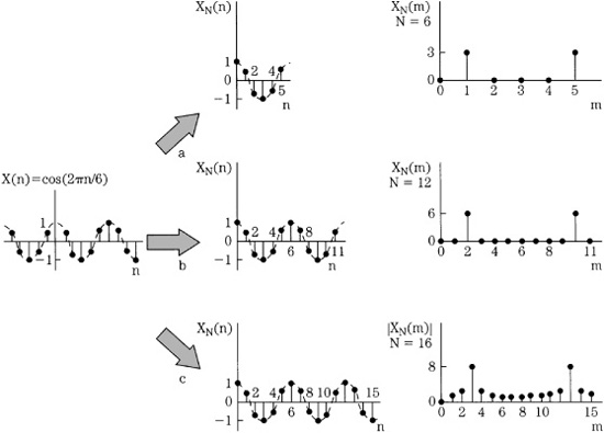
FIGURE 17.6 Example of a periodic signal applied to an N-point DFT for three different values of N. Greater spectral resolution is obtained as N is increased. When N is not equal to an integral number of waveform periods, spectral leakage occurs. (Van den Enden and Verhoeckx, 1985)
The DFT is computation-intensive, requiring N2 complex multiplications and N(N - 1) complex additions. The DFT is often generated with the fast Fourier transform (FFT), a collection of fast and efficient algorithms for spectral computation that takes advantage of computational symmetries and redundancies in the DFT. The FFT requires Nlog2N computations, 100 times fewer than DFT. The FFT can be used when N is an integral power of 2; zero samples can be padded to satisfy this requirement. The FFT can also be applied to a sequence length that is a product of smaller integer factors. The FFT is not another type of transformation, but rather an efficient method of calculating the DFT. The FFT recursively decomposes an N-point DFT into smaller DFTs. This number of short-length DFTs are calculated, then the results are combined. The FFT can be applied to various calculation methods and strategies, including the analysis of signals and filter design.
The FFT will transform a time series, such as the impulse response of a network, into the real and imaginary parts of the impulse response in the frequency domain. In this way, the magnitude and phase of the network’s transfer function can be obtained. An inverse FFT can produce a time-domain signal. FFT filtering is accomplished through multiplication of spectra. The impulse response of the filter is transformed to the frequency domain. Real and imaginary arrays, obtained by FFT transformation of overlapping segments of the signal, are multiplied by filter arrays, and an inverse FFT produces a filtered signal. Because the FFT can be efficiently computed, it can be used as an alternative to time-domain convolution if the overall number of multiplications is fewer.
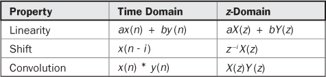
TABLE 17.1 Equivalent properties of discrete signals in the time domain and z-domain.
The z-transform operates on discrete signals in the same way that the Laplace transform operates on continuous signals. In the same way that the Laplace transform is a generalization of the Fourier transform, the z-transform is a generalization of the DFT. Whereas the Fourier transform operates on a particular complex value e−j, the z-transform operates with any complex value. When z = ej, the z-transform is identical to the Fourier transform. The DFT is thus a special case of the z-transform. The z-transform of a sequence x(n) is defined as:
![]()
where z is a complex variable and z−1 represents a unit delay element. The z-transform has an inverse transform, often obtained through a partial fraction expansion.
Whereas the DFT is used for literal operations, the z-transform is a mathematical tool used in digital signal processing theory. Several basic properties govern the z-domain. A linear combination of signals in the time domain is equivalent to a linear combination in the z-domain. Convolution in the time domain is equivalent to multiplication in the z-domain. For example, we could take the z-transform of the convolution equation, such that the z-transform of an input multiplied by the z-transform of a filter’s impulse response is equal to the z-transform of the filter’s output. In other words, the ratio of the filter output transform to the filter input transform (that is, the transfer function H(z)) is the z-transform of the impulse response. Furthermore, this ratio, the transfer function H(z), is a fixed function determined by the filter. In the z-domain, given an impulse input, the transfer function equals the output. Furthermore, a shift in the time domain is equivalent to multiplication by z raised to a power of the length (in samples) of the shift. These properties are summarized in Table 17.1. For example, the z-transforms of x(n) and y(n) are X(z) and Y(z), respectively.
Unit Circle and Region of Convergence
The Fourier transform of a discrete signal corresponds to the z-transform on the unit circle in the z-plane. The equation z = ej defines the unit circle in the complex plane. The evaluation of the z-transform along the unit circle yields the function’s frequency response.
The variable z is complex, and X(z) is the function of the complex variable. The set of z in the complex plane for which the magnitude of X(z) is finite is said to be in the region of convergence. The set of z in the complex plane for which the magnitude of X(z) is infinite is said to diverge, and is outside the region of convergence. The function X(z) is defined over the entire z-plane but is only valid in the region of convergence. The complex variable s is used to describe complex frequency; this is a function of the Laplace transform. S variables lie on the complex s-plane. The s-plane can be mapped to the z-plane; vertical lines on the s- plane map as circles in the z-plane.
Because there is a finite number of samples, practical systems must be designed within the region of convergence. The unit circle is the smallest region in the z-plane that falls within the region of convergence for all finite stable sequences. Poles must be placed inside the unit circle on the z-plane for proper stability. Improper placement of the poles constitutes an instability.
Mapping from the s-plane to the z-plane is an important process. Theoretically, this function allows the designer to choose an analog transfer function and find the z-transform of that function. Unfortunately, the s-plane generally does not map into the unit circle of the z-plane. Stable analog filters, for example, do not always map into stable digital filters. This is avoided by multiplying by a transform constant, used to match analog and digital frequency response. There is also a nonlinear relationship between analog and digital break frequencies that must be accounted for. The nonlinearities are known as warping effects and the use of the constant is known as pre-warping the transfer function.
Often, a digital implementation can be derived from an existing analog representation. For example, a stable analog filter can be described by the system function H(s). Its frequency response is found by evaluating H(s) at points on the imaginary axis of the s-plane. In the function H(s), s can be replaced by a rational function of z, which will map the imaginary axis of the s-plane onto the unit circle of the z-plane. The resulting system function H(z) is evaluated along the unit circle and will take on the same values of H(s) evaluated along its imaginary axis.
Poles and Zeros
Summarizing, the transfer function H(z) of a linear, time-invariant discrete-time filter is defined to be the z-transform of the impulse response h(n). The spectrum of a function is equal to the z-transform evaluated on the unit circle. The transfer function of a digital filter can be written in terms of its z-transform; this permits analysis in terms of the filter’s poles and zeros. The zeros are the roots of the numerator’s polynomial of the transfer function of the filter, and the poles are the denominator’s roots. Mathematically, zeros make H(z) = 0, and poles make H(z) nonanalytic. When the magnitude of H(z) is plotted as a function of z, poles appear at a distance above the z-plane and zeros touch the z-plane. One might imagine the flat z-plane and above it a flexible contour, the magnitude transfer function, passing through the poles and zeros, with peaks on top of poles, and valleys centered on zeros. Tracing the rising and falling of the contour around the unit circle yields the frequency response. For example, the gain of a filter at any frequency can be measured by the magnitude of the contour. The phase shift at any frequency is the angle of the complex number that represents the system’s response at that frequency.
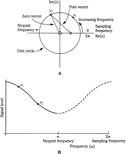
FIGURE 17.7 The frequency response of a filter can be obtained from the pole/zero plot. The amplitude of the frequency response (for example, at points a1 and a2) is obtained by dividing the magnitude of the zero vector by that of the pole vector at those points on the unit circle. A. An example of a z-plane plot of a lowpass filter, showing the pole and zero locations. B. Analysis of the z-plane plot reveals the filter’s lowpass frequency response.
If we plot ∣z∣ = 1 on the complex plane, we get the unit circle; ∣z∣ > 1 specifies all points on the complex plane that lie outside the unit circle; and ∣z∣ < 1 specifies all points inside it. The z-transform of a sequence can be represented by plotting the locations of the poles and zeros on the complex plane.
Figure 17.7A shows an example of a z-plane plot. Among other approaches, the response can be analyzed by examining the relationships between the pole and zero vectors. In the z-plane, angular frequency is represented as an angle, with a rotation of 360° corresponding to the sampling frequency. The Nyquist frequency is thus located at ![]() in the figure. The example shows a single pole (
in the figure. The example shows a single pole (![]() ) and zero (o). The corresponding frequency response from 0 to the Nyquist frequency is seen to be that of a lowpass filter, as shown in Fig. 17.7B. The amplitude of the frequency response can be determined by dividing the magnitude of the zero vector by that of the pole vector. For example, points a1 and a2 are plotted on the unit circle, and on the frequency response graph. Similarly, the phase response is the difference between the pole vector’s angle (from = 0 radians) and the zero vector’s angle. As the positions of the pole and zero are varied, the response of the filter changes. For example, if the pole is moved along the negative real axis, the filter’s frequency response changes to that of a highpass filter.
) and zero (o). The corresponding frequency response from 0 to the Nyquist frequency is seen to be that of a lowpass filter, as shown in Fig. 17.7B. The amplitude of the frequency response can be determined by dividing the magnitude of the zero vector by that of the pole vector. For example, points a1 and a2 are plotted on the unit circle, and on the frequency response graph. Similarly, the phase response is the difference between the pole vector’s angle (from = 0 radians) and the zero vector’s angle. As the positions of the pole and zero are varied, the response of the filter changes. For example, if the pole is moved along the negative real axis, the filter’s frequency response changes to that of a highpass filter.
Some general observations: zeros are created by summing input samples, and poles are created by feedback. A filter’s order equals the number of poles or zeros it exhibits, whichever is greater. A filter is stable only if all its poles are inside the unit circle of the z-plane. Zeros can lie anywhere. When all zeros lie inside the unit circle, the system is called a minimum-phase network. If all poles are inside the unit circle and all zeros are outside, and if poles and zeros are always reflections of one another in the unit circle, the system is a constant-amplitude, or all-pass network. If a system has zeros only, except for the origin, and they are reflected in pairs in the unit circle, the system is phase-linear. No real function can have more zeros than poles. When the coefficients are real, poles and zeros occur in complex conjugate pairs; their plot is symmetrical across the real z-axis. The closer its location to the unit circle, the greater the effect of each pole and zero on frequency response.
DSP Elements
Successful DSP applications require sophisticated hardware and software. However, all DSP processing can be considered in three simple processing operations: summing, multiplication, and time delay, as shown in Fig. 17.8. With summing, multiple digital values are added to produce a single result. With multiplication, a gain change is accomplished by multiplying the sample value by a coefficient. With time delay (n - 1), a digital value is stored for one sample period. The delay element (realized with shift registers or memory locations) is alternatively notated as z-1 because a delay of one sampling period in the time domain corresponds to multiplication by z-1 in the z-domain; thus z-1x(n) = x(n - 1). Delays can be cascaded, for example, a z-2 term describes a two-sample (n - 2) delay. Although it is usually most convenient to operate with sample numbers, the time of a delay can be obtained by taking nT, where T is the sampling interval. Figure 17.9 shows two examples of simple networks and their impulse responses (see also Fig. 17.1B). LTD systems such as these are completely described by the impulse response.
In practice, these elemental operations are performed many times for each sample, in specific configurations depending on the desired result. In this way, algorithms can be devised to perform operations useful to audio processing such as reverberation, equalization, data reduction, limiting, and noise removal. Of course, for real-time operation, all processing for each sample must be completed within one sampling period.
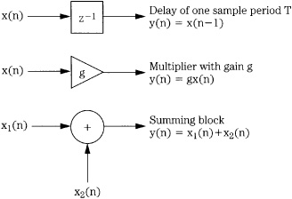
FIGURE 17.8 The three basic elements in any DSP system are delay, multiplication, and summation. They are combined to accomplish useful processing.
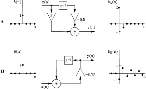
FIGURE 17.9 LTD systems can be characterized by their impulse responses. A. A simple nonrecursive system and its impulse response. B. A simple recursive system and its impulse response. (Van den Enden and Verhoeckx, 1985)
Digital Filters
Filtering (or equalization) is important in many audio applications. Analog filters using both passive and active designs shape the signal’s frequency response and phase, as described by linear time-invariant differential equations. They describe the system’s performance in the time domain. With digital filters, each sample is processed through a transfer function to affect a change in frequency response or phase. Operation is generally described in linear shift-invariant difference equations; they define how the discrete time signal behaves from moment to moment in the time domain. At an infinitely high sampling rate, these equations would be identical to those used to describe analog filters. Digital filters can be designed from analog filters; such impulse-invariant design is useful for lowpass filters with a cutoff frequency far below the sampling rate. Other filter designs make use of transformations to convert characteristics of an analog filter to a digital filter. These transformations map the frequency range of the analog domain into the digital range, from 0 Hz to the Nyquist frequency.
A digital filter can be represented by a general difference equation:
y(n) + b1y(n − 1) + b2y(n − 2)+ … + bNy(n − N)
= a0x(n) + a1x(n − 1) + a2x(n − 2) + … + aMx(n − M)
More efficiently, the equation can be written as:
![]()
where x is the input signal, y is the output signal, the constants ai and bi are the filter coefficients, and n represents the current sample time, the variable in the filter’s equation. A difference equation is used to represent y(n) as a function of the current input, previous inputs, and previous outputs. The filter’s order is specified by the maximum time duration (in samples) used to generate the output. For example, the equation:
y(n) = x(n) − y(n − 2) + 2x(n − 2) + x(n −3)
is a third-order filter.
To implement a digital filter, the z-transform is applied to the difference equation so that it becomes:
![]()
where z-i is a unit of delay i in the time domain. Rewriting the equation, the transfer function H(z) can be determined by:
As noted, the transfer function can be used to identify the filter’s poles and zeros. Specifically, the roots (values that make the expression zero) of the numerator identify zeros, and roots of the denominator identify poles. Zeros constitute feed-forward paths and poles constitute feedback paths. By tracing the contour along the unit circle, the frequency response of the filter can be determined.
A filter is canonical if it contains the minimum number of delay elements needed to achieve its output. If the values of the coefficients are changed, the filter’s response is altered. A filter is stable if its impulse response approaches zero as n goes to infinity. Convolution provides the means for implementing a filter directly from the impulse response; convolving the input signal with the filter impulse response gives the filtered output. In other words, convolution acts as the difference equation, and the impulse response acts in place of the difference equation coefficients in representing the filter. The choice of using a difference equation or convolution in designing a filter depends on the filter’s architecture, as well as the application.
FIR Filters
As noted, the general difference equation can be written as:
y(n) + b1y(n − 1) + b2y(n − 2) + … + bNy(n − N)
= a0x(n) + a1x(n − 1) + a2x(n − 2) + … + aMx(n − M)
Consider the general difference equation without bi terms:
![]()
and its transfer function in the z domain:
![]()
There are no poles in this equation; hence there are no feedback elements. The result is a nonrecursive filter. Such a filter would take the form:
y(n) = ax(n) + bx(n − 1) + cx(n − 2) + dx(n − 3) + …
Any filter operating on a finite number of samples is known as a finite impulse response (FIR) filter. As the name FIR implies, the impulse response has finite duration. Furthermore, an FIR filter can have only zeros outside the origin, it can have a linear phase (symmetrical impulse response). In addition, it responds to an impulse once, and it is always stable. Because it does not use feedback, it is called a nonrecursive filter. A nonrecursive structure is always an FIR filter; however, an FIR filter does not always use a nonrecursive structure.
Consider this introduction to the workings of FIR filters: we know that large differences between samples are indicative of high frequencies and small differences are indicative of low frequencies. A filter changes the differences between consecutive samples. The digital filter described by y(n) = 0.5[x(n) + x(n - 1)] makes the current output equal to half the current input plus half the previous input. Suppose this sequence is input: 1, 8, 6, 4, 1, 5, 3, 7; the difference between consecutive samples ranges from 2 to 7. The first two numbers enter the filter and are added and multiplied: (1 + 8)(0.5) = 4.5. The next computation is (8 + 6)(0.5) = 7.0. After the entire sequence has passed through the filter the sequence is: 4.5, 7, 5, 2.5, 3, 4, 5. The new intersample difference ranges from 0.5 to 2.5; this filter averages the current sample with the previous sample. This averaging smoothes the output signal, thus attenuating high frequencies. In other words, the circuit is a lowpass filter.
More rigorously, the filter’s difference equation is:
y(n) = 0.5[x(n) + x(n − 1)]
Transformation to the z-domain yields:
Y(z) = 0.5[X(z) + z−1X(z)]
The transfer function can be written as:
![]()
This indicates a zero at z = -1 and a pole at z = 0, as shown in Fig. 17.10A. Tracing the unit circle, the filter’s frequency response is shown in Fig. 17.10B; it is a lowpass filter. Finally, the difference equation can be realized with the algorithm shown in Fig. 17.10C.
Another example of a filter is one in which the output is formed by subtracting the past input from the present, and dividing by 2. In this way, small differences between samples (low-frequency components) are attenuated and large differences (high-frequency components) are accentuated. The equation for this filter is only slightly different from the previous example:

FIGURE 17.10 An example showing the response and structure of a digital lowpass FIR filter. A. The pole and zero locations of the filter in the z-plane. B. The frequency response of the filter. C. Structure of the lowpass filter.
y(n) = 0.5[x(n) − x(n − 1)]
Transformation to the z-plane yields:
Y(z) = 0.5[X(z) − z-1 X(z)]
The transfer function can be written as:
![]()
This indicates a zero at z = 1 and a pole at z = 0, as shown in Fig. 17.11A. Tracing the unit circle, the filter’s frequency response is shown in Fig. 17.11B; it is a highpass filter. The difference equation can be realized with the algorithm shown in Fig. 17.11C. This highpass filter’s realization differs from that of the previous lowpass filter’s realization only in the -1 multiplier. In both of these examples, the filter must store only one previous sample value. However, a filter could be designed to store a large (but finite) number of samples for use in calculating the response.
An FIR filter can be constructed as a multi-tapped digital filter, functioning as a building block for more sophisticated designs. The direct-form structure for realizing an FIR filter is shown in Fig. 17.12. This structure is an implementation of the convolution sum. To achieve a given frequency response, the impulse response coefficients of an FIR filter must be calculated. Simply truncating the extreme ends of the impulse response to obtain coefficients would result in an aperture effect and Gibbs phenomenon. The response will peak just below the cutoff frequency and ripples will appear in the passband and stopband. All digital filters have a finite bandwidth; in other words, in practice the impulse response must be truncated. Although the Fourier transform of an infinite (ideal) impulse response creates a rectangular pulse, a finite (real-world) impulse response creates a function exhibiting Gibbs phenomenon. This is not ringing as in analog systems, but the mark of a finite bandwidth system.
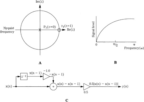
FIGURE 17.11 An example showing the response and structure of a digital highpass FIR filter. A. The pole and zero locations of the filter in the z-plane. B. The frequency response of the filter. C. Structure of the highpass filter.
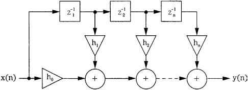
FIGURE 17.12 The direct-form structure for realizing an FIR filter. This multi-tapped structure implements the convolution sum.
Choice of coefficients determines the phase linearity of the resulting filter. For many audio applications, linear phase is important; the filter’s constant delay versus frequency linearizes the phase response and results in a symmetrical output response. For example, the steady-state response of a phase linear system to a square-wave input displays center and axial symmetry. When a system’s phase response is nonlinear, the step response does not display symmetry.
The length of the impulse to be considered depends on the frequency response and filter ripple. It is important to provide a smooth transition between samples that are relevant and those that are not. In many applications, the filter coefficients are multiplied by a window function. A window can be viewed as a finite weighting sequence used to modify the infinite series of Fourier coefficients that define a given frequency response. The shape of a window affects the frequency response of the signal correspondingly by the frequency response of the window itself. As noted, multiplication in the time domain is equivalent to convolution in the frequency domain. Multiplying a time-domain signal by a time-domain window is the same as convolving the signals in the frequency domain. The effect of a window on a signal’s frequency response can be determined by examining the DFT of the window.
Many DSP applications involve operation on a finite set of samples, truncated from a larger data record; this can cause side effects. For example, as noted, the difference between the ideal and actual filter lengths yields Gibbs phenomenon overshoot at transitions in the transfer function in the frequency domain. This can be reduced by multiplying the coefficients by a window function, but this also can change the transition bands of the transfer function.
For example, a rectangular window function can be used to effectively gate the signal. The window length can only take on integer values, and the window length must be an integer multiple of the input period. The input signal must repeat itself over this integer number of samples. The method works well because the spacing of the nulls in the window transform is exactly the same as the spacing of the harmonics of the input signal. However, if the integer relationship is broken, and there is not an exact number of periods in the window, spectrum nulls do not correspond to harmonic frequencies and there is spectral leakage.
Some window functions are used to overcome spectral leakage. They are smoothly tapered to gradually reduce the amplitude of the input signal at the endpoints of the data record. They attenuate spectral leakage according to the energy of spectral content outside their main lobe.
Alternatively, the desired response can be sampled, and the discrete Fourier transform coefficients computed. These are then related to the desired impulse response coefficients. The frequency response can be approximated, and the impulse response calculated from the inverse discrete Fourier transform. Still another approach is to derive a set of conditions for which the solution is optimal, using an algorithm providing an approximation, with minimal error, to the desired frequency response.
IIR Filters
The general difference equation contains y(n) components that contribute to the output value. These are feedback elements that are delayed by a unit of time i, and describe a recursive filter. The feedback elements are described in the denominator of the transfer function. Because the roots cause H(z) to be undefined, certain feedback could cause the filter to be unstable. The poles contribute an exponential sequence to each pole’s impulse response. When the output is fed back to the input, the output in theory will never reach zero; this allows the impulse to be infinite in duration. This type of filter is known as an infinite impulse response (IIR) filter.
Feedback provides a powerful method for recalling past samples. For example, an exponential time-average filter adds the current input sample to the last output (as opposed to the previous sample) and divides the result by 2. The equation describing its operation is: y(n) = x(n) + 0.5y(n - 1). This yields an exponentially decaying response in which each next output sample is one-half the previous sample value. The filter is called an infinite impulse response filter because of its infinite memory. In theory, the impulse response of an IIR filter lasts for an infinite time; its response never decays to zero. This type of filter is equivalent to an infinitely long FIR filter where:
y(n) = x(n) + 0.5x(n − 1) + 0.25x(n − 2) + 0.125x(n − 3)+ …. +(0.5)Mx(n − M)
In other words, the filter adds one-half the current sample, one-fourth the previous sample, and so on. The impulse response of a practical FIR filter decays exponentially, but it has a finite length, thus cannot decay to zero.
In general, an IIR filter can be described as:
y(n) = ax(n) + by(n − 1)
When the value of b is increased relative to a, the lowpass filtering is augmented; that is, the cutoff frequency is lowered. The value of b must always be less than unity or the filter will become unstable; the signal level will increase and overflow will result.
An IIR filter can have both poles and zeros, can introduce phase shift, and can be unstable if one or more poles lie on or outside the unit circle. Generally, an all-pole filter is an IIR filter. IIR filters cannot achieve linear phase (the impulse response is asymmetrical) except in the case when all poles in the transfer function lie on the unit circle. This is realized when the filter consists of a number of cascaded first-order sections. Because the output of an IIR is fed back as an input (with a scaling element), it is called a recursive filter. An IIR filter always has a recursive structure, but filters with a recursive structure are not always IIR filters. Any feedback loop must contain a delay element. Otherwise, the value of a sample would have to be known before it is calculated—an impossibility.
Consider the IIR filter described by the equation:
y(n) = x(n) − x(n − 2) − 0.25y(n − 2)
It can be rewritten as:
y(n) + 0.25y(n − 2) = x(n) − x(n − 2)
Transformation to the z-plane yields:
Y(z) + 0.25z-2Y(z) = X(z) − z-2X(z)
The transfer function is:
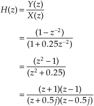
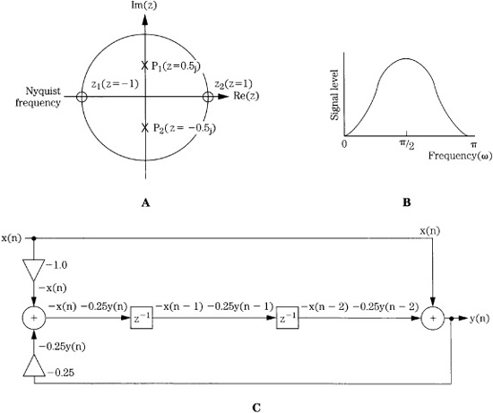
FIGURE 17.13 An example showing the response and structure of a digital bandpass IIR filter. A. The pole and zero locations of the filter in the z-plane. B. The frequency response of the filter. C. Structure of the bandpass filter.
There are zeros at z = ±1 and conjugate poles on the imaginary axis at z = ±0.5j, as shown in Fig. 17.13A. The frequency response can be graphically determined by dividing the product of zero-vector magnitudes by the product of the pole-vector magnitudes; (phase response is the difference between the sum of their angles). The resulting bandpass frequency response is shown in Fig. 17.13B. A realization of the filter is shown in Fig. 17.13C. Delay elements have been combined to simplify the design. Similarly, the difference equation y(n) = x(n) + x(n - 2) + 0.25y(n - 2) is also an IIR filter. The development of its pole/zero plot, frequency response, and realization are left to the ambition of the reader.
In general, it is easier to design FIR filters with linear phase and stable operation than IIR filters with the same characteristics. However, IIR filters can achieve a steeper roll-off than an FIR filter for a given number of coefficients. FIR filters require more stages, and hence greater computation, to achieve the same result. As with any digital processing circuit, noise must be considered. A filter’s type, topology, arithmetic, and coefficient values all determine whether meaningful error will be introduced. For example, the exponential time-average filter described above will generate considerable error if the value of b is set close to unity, for a low cutoff frequency.
Filter Applications
An example of second-order analog filter is shown in Fig. 17.14A, and an IIR filter is shown in Fig. 17.14B; this is a biquadratic filter section. Coefficients determine the filter’s response; in this example, with appropriate selection of the five multiplication coefficients, highpass, lowpass, bandpass, and shelving filters can be obtained. A digital audio processor might have several of these sections at its disposal. By providing a number of presets, users can easily select frequency response, bandwidth, and phase response of a filter. In this respect, a digital filter is more flexible than an analog filter that has relatively limited operating parameters. However, a digital filter requires considerable computation, particularly in the case of swept equalization. As the center frequency is moved, new coefficients must be calculated—not a trivial task. To avoid quantization effects (sometimes called zipper noise), filter coefficients and amplitude scaling coefficients must be updated at a theoretical rate equal to the sampling rate; in practice, an update rate equal to one-half or one-fourth the sampling rate is sufficient. To accomplish even this, coefficients are often obtained through linear interpolation. The range must be limited to ensure that filter poles do not momentarily pass outside the unit circle, causing transient instability.
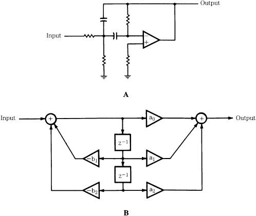
FIGURE 17.14 A comparison of second-order analog and digital filters. A. A second-order analog filter. B. An IIR biquadratic second-order filter section. (Tydelski, 1988)
Adaptive filters automatically adjust their parameters according to optimization criteria. They do not have fixed coefficients; instead, values are calculated during operation. Adaptive filters thus consist of a filter section and a control unit used to calculate coefficients. Often, the algorithm used to compute coefficients attempts to minimize the difference between the output signal and a reference signal. In general, any filter type can be used, but in practice, adaptive filters often use a transversal structure as well as lattice and ladder structures. Adaptive filters are used for applications such as echo and noise cancelers, adaptive line equalizers, and prediction.
A transversal filter is an FIR filter in which the output value depends on both the input value and a number of previous input values held in memory. Inputs are multiplied by coefficients and summed by an adder at the output. Only the input values are stored in delay elements; there are no feedback networks; hence it is an example of a nonrecursive filter. As described in Chap. 4, this architecture is used extensively to implement lowpass filtering with oversampling.
In practice, digital oversampling filters often use a cascade of FIR filters, designed so the sampling rate of each filter is a power of 2 higher than the previous filter. The number of delay blocks (tap length) in the FIR filter determines the passband flatness, transition band slope, and stopband rejection; there are M + 1 taps in a filter with M delay blocks. Many digital filters are dedicated chips. However, general purpose DSP chips can be used to run custom filter programs.
The block diagram of a dedicated digital filter (oversampling) chip is shown in Fig. 17.15. It demonstrates the practical implementation of DSP techniques. A central processor performs computation while peripheral circuits accomplish input/output and other functions. The filter’s characteristic is determined by the coefficients stored in ROM; the multiplier/accumulator performs the essential arithmetic operations; the shifter manages data during multiplication; the RAM stores intermediate computation results; a microprogram stored in ROM controls the filter’s operation. The coefficient word length determines filter accuracy and stopband attenuation. A filter can have, for example, 293 taps and a 22-bit coefficient; this would yield a passband that is flat to within ±0.00001 dB, with a stopband suppression greater than 120 dB. Word length of the audio data increases during multiplication; truncation would result in quantization error thus the data must be rounded or dithered. Noise shaping can be applied at the accumulator, using an IIR filter to redistribute the noise power, primarily placing it outside the audio band. Noise shaping is discussed in Chap. 18.
FIGURE 17.15 An example showing the functional elements of a dedicated digital filter (oversampling) chip.
Sources of Errors and Digital Dither
Unless precautions are taken, the DSP computation required to process an audio signal can add noise and distortion to the signal. In general, errors in digital processors can be classified as coefficient, limit cycle, overflow, truncation, and round-off errors. Coefficient errors occur when a coefficient is not specified with sufficient accuracy. For example, a resolution of 24 bits or more is required for computations on 16-bit audio samples. Limit cycle error might occur when a signal is removed from a filter, leaving a decaying sum. This decay might become zero or might oscillate at a constant amplitude, a condition known as limit cycle oscillation. This effect can be eliminated, for example, by offsetting the filter’s output so that truncation always produces a zero output.
Overflow occurs when a register length is exceeded, resulting in a computational error. In the case of wraparound, when a 1 is added to the maximum value positive two’s complement number, the result is the maximum value negative number. In short, the information has overflowed into a nonexistent bit. The drastic change in the amplitude of the output waveform would yield a loud pop if applied to a loudspeaker. To prevent this, saturating arithmetic can be used so that when the addition of two positive numbers would result in a negative number, the maximum positive sum is substituted instead. This results in clipping—a more satisfactory, or at least more benign, alternative. Alternatively, designers must provide sufficient digital headroom.
Truncation and round-off errors occur whenever the word length of a computed result is limited. Errors accumulate both inside the processor during calculation, and when word length is reduced for output through a D/A converter. However, A/D conversion always results in quantization error, and computation error can appear in different guises. For example, when two n-bit numbers are multiplied, the number of output bits will be 2n - 1. Thus, multiplication almost doubles the number of bits required to represent the output. Although many hardware multipliers can perform double-precision computation, a finite word length must be maintained following multiplication, thus limiting precision. Discarded data results in an error analogous to that of A/D quantization. To be properly modeled, multiplication must be followed by quantization; multiplication does not introduce error, but inability to keep the extra bits does. It is important to note that unnecessary cumulative dithering should be avoided in interim calculations.
Rather than truncate a word, for example, following multiplication, the value can be rounded; that is, the word is taken to the nearest available value. This results in a peak error of 1/2 LSB, and an rms value of 1/(12)1/2, or 0.288 LSB. This round-off error will accumulate over successive calculations. In general, the number of calculations must be large for significant error to occur. However, in addition, dither information can be lost during computation. For example, when a properly dithered 16-bit word is input to a 32-bit processor, even though computation is of high precision, the output signal might be truncated to 16 bits for conversion through the output D/A converter. For example, a 16-bit signal that is delayed and scaled by a 12-dB attenuation would result in a 12-bit undithered signal. To overcome this, digital dithering to the resolution of the next processing (or recording) stage should be used in a computation.
To apply digital dithering, a pseudo-random number of the appropriate magnitude is added to each sample and then the new LSB is rounded up or down to the nearest quantization interval according to value of the portion to be discarded. In other words, a logical 1 is added to the new LSB and the lower portion is discarded, or the lower portion is simply discarded. The lower bit information thus modulates the new LSB and provides the linearizing benefit of dithering. A different pseudo-random number is used for each audio channel. To duplicate the effects of analog dither, two’s complement digital dither values should be used to provide a bipolar signal with an average zero value. In some cases, noise shaping is also applied at this stage. Bipolar pseudo-random noise and a D/A converter can be used to generate analog dither.
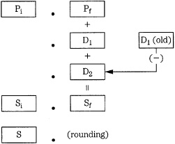
FIGURE 17.16 An example of digital redithering used during a truncation or rounding computation. (Vanderkooy and Lipshitz, 1989)
As an example of digital dithering, consider a 20-bit resolution signal that must be dithered to 16 bits. IIR and noise-shaping filters with digital feedback can exhibit limit cycle oscillations with low-level signals if gain reduction or certain equalization processing (resulting in gain changes) is performed; digital dither can be used to randomize these cycles.
John Vanderkooy and Stanley Lipshitz have shown that truncated or rounded digital words can be redithered with rectangular pdf or triangular pdf fractional numbers, as shown in Fig. 17.16. A rectangular pdf dither word D1 is added to a digital audio word with integer part Pi and fractional part Pf. The carry bit dithers the rounding process in the same way that 1 LSB analog rectangular pdf dither affects an A/D converter. When a statistically independent rectangular pdf dither D2 is added, triangular pdf dither results. This triangular pdf dither noise power is Q2/6 and rounding noise power is Q2/12 so the total noise power is Q2/4. The final sum has integer part Si and fractional part Sf, which become S upon rounding.
In cases of gain fading, triangular pdf appears to be a better choice than rectangular pdf because it eliminates noise modulation as well as distortion, at the expense of a slightly higher noise floor. To minimize audibility of this noise penalty, highpass triangular pdf dither can be most appropriate in rounding. The triangular pdf statistics are not changed. However, dither samples are correlated. Average dither noise power is Q2/6, with no noise at 0 Hz and double the average value at the Nyquist frequency. Hence the term: highpass dither. This shaping becomes more pronounced with noise increasingly shifted outside the audio band, as the oversampling ratio is increased, for example, by eight times. The audible effect of a noise penalty is lessened when oversampling is used because in-band noise is relatively decreased proportional to the oversampling rate. Further reduction of the Q2/12 requantization noise power can be achieved through noise-shaping circuits, as described in Chap. 18.
As noted, the problem of error sources is applicable to both audio samples as well as the computations used to determine other system operators, such as filter coefficients. For example, improperly computed filter coefficients could shift the locations of poles and zeros, thus altering the characteristics of the response. In some cases, an insufficiently defined coefficient can cause a stable IIR filter to become unstable. On the other hand, the quantization of filter coefficients will not affect the linear operation of a circuit, or introduce artifacts that are affected by the input signal or that vary with time. The effect of coefficient errors in a filter is generally determined by the number of coefficients determining the location of each pole and zero. The fewer the coefficients, the lower the sensitivity. However, when poles and zeros are placed in locations where they are few, the effect of errors is greater.
DSP Integrated Circuits
A DSP chip is a specialized hardware device that performs digital signal processing under the control of software algorithms. DSP chips are stand-alone processors, often independent of host CPUs (central processing units), and are specially designed for operations used in spectral and numerical applications. For example, large numbers of multiplications are possible, as well as special addressing modes such as bit-reverse and circular addressing. When memory and input/output circuits are added, the result is an integrated digital signal processor. Such a general purpose DSP chip is software programmable, and thus can be used for a variety of signal-processing applications. Alternatively, a custom signal processor can be designed to accomplish a specific task.
Digital audio applications require long word lengths and high operating speeds. To prevent distortion from rounding error, the internal word length must be 8 to 16 bits longer than the external word. In other words, for high-quality applications, internal processing of 24 to 32 bits or more is required. For example, a 24-bit DSP chip might require a 56-bit accumulator to prevent overflow when computing long convolution sums.
Processor Architecture
DSP chips often use a pipelining architecture so that several instructions can be paralleled. For example, with pipelining, a fetch (fetch instruction from memory and update program counter), decode (decode instruction and generate operand address), read (read operand from memory), and execute (perform necessary operations) can be effectively executed in one clock cycle. A pipeline manager, aided by proficient user programming, helps ensure efficient processing.
DSP chips, like all computers, are composed of input and output devices, an arithmetic logic unit, a control unit, and memory, interconnected by buses. All computers originally used a single sequential bus (von Neumann architecture), shared by data, memory addresses, and instructions. However, in a DSP chip a particularly large number of operations must be performed quickly for real-time operation. Thus, parallel bus structures are used (such as the Harvard architecture) that store data and instructions in separate memories and transfer them via separate buses. For example, a chip can have separate buses for program, data, and direct memory access (DMA), providing parallel program fetches, data reads, as well as DMA operations with slower peripherals.
A block diagram of a general purpose DSP chip is shown in Fig. 17.17; many DSP chips follow a similar architecture. The chip has seven components: multiply-accumulate unit, data address generator, data RAM, coefficient RAM, coefficient address generator, program control unit, and program ROM. Three buses interconnect these components: data bus, coefficient bus, and control bus. In this example, the multiplier is asymmetrical; it multiplies 24-bit sample words by 12-bit coefficient words. The result of multiplication is carried out to 36 bits. For dynamic compression, the 12-bit words containing control information are derived from the signal itself; two words could be taken together to provide double precision when necessary. A 40-bit adder is used in this example. This adds the results of multiplications to other results stored in the 40-bit accumulator. Following addition in the arithmetic logic unit (ALU), words must be quantized to 24 bits before being placed on the data bus. Different methods of quantization can be applied.
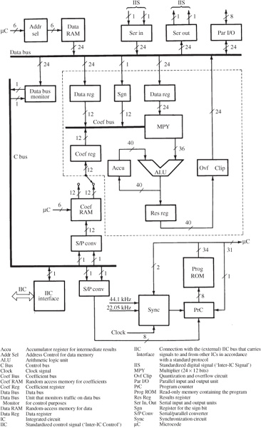
FIGURE 17.17 Block diagram of a digital signal processor chip. The section surrounded by a dashed line is the arithmetic unit where computation occurs. Independent buses are used for data, coefficients, and control.
Coefficients are taken from the coefficient RAM, loaded with values appropriate to the task at hand, and applied to the coefficient bus. Twenty-four-bit data samples are moved from the data bus to two data registers. Parallel and serial inputs and outputs, and data memory can be connected to the data bus. This short memory (64 words by 24 bits, in this case) performs the elementary delay operation. As noted, to speed multiple multiplications, pipelining is provided. Necessary subsequent data is fed to intermediate registers simultaneously with operations performed on current data.
Fixed Point and Floating Point
DSP chips are designed according to two arithmetic types, fixed point and floating point, which define the format of the data they operate on. Fixed-point (or fixed-integer) chips use two’s complement, binary integer data. Floating-point chips use integer and floating-point numbers (represented as a mantissa and exponent). The dynamic range of a fixed-point chip is based on its word length. Data must be scaled to prevent overflow; this can increase programming complexity. The scientific notation used in a floating-point chip allows a larger dynamic range, without overflow problems. However, the resolution of floating point representation is limited by the word length of the exponent.
Many factors are considered by programmers when deciding which DSP chip to use in an application. These include cost, programmability, ease of implementation, support, availability of useful software, availability of internal legacy software, time to market, marketing impact (for example, the customer’s perception of 24-bit versus 32-bit), and sound quality. As Brent Karley notes, programming style and techniques are both critical to the sound quality of a given audio implementation. Moreover, the hardware platform can also affect sound quality. Neither can be ignored when developing high-quality DSP programs. The Motorola DSP56xxx series of processors is an example of a fixed-point architecture, and the Analog Devices SHARC series is an example of a floating-point architecture. Conventional personal computer processors can perform both kinds of calculations.
Three principal processor types are widely used in DSP-based audio products: 24-bit fixed point, 32-bit fixed point, and 32-bit floating point (24 mantissa bits with 8 exponent bits). Each variant of precision and architecture has advantages and disadvantages for sound quality. When comparing 32-bit fixed and 24-bit fixed, with the same program running on two DSP chips of the same architecture, the higher precision DSP will obviously provide higher quality audio. However, DSP chips often do not use the same architecture and do not support the same implementation of any given algorithm. It is thus possible for a 24-bit fixed-point DSP chip to exceed the sound quality of a 32-bit fixed-point chip. For example, some DSP chips have hardware accelerators that can off-load some processing chores to free up processing resources that can be allocated to audio quality improvements or extra features. Programming methods such as double-precision arithmetic and truncation-reduction methods may be implemented to improve quality. Optimization programming methods can be performed on any of the available DSP architectures, but are often not implemented (or only in limited numbers) because of processing or memory limitations.
For higher-quality audio implementations, a 24-bit fixed-point DSP chip can implement double-precision filtering or processing in strategic components of a given algorithm to improve the sound quality beyond that of a 32-bit fixed-point DSP chip. The combination of two 24-bit numbers into one 48-bit integer allows very high-fidelity processing. This is possible in some cases due to the higher processing power available in some 24-bit DSP chips over less efficient 32-bit DSP chips. Some manufacturers carefully hand-optimize their implementations to exceed the sound quality of competitors using 32-bit fixed-point DSP chips. Chip manufacturers often provide different versions of audio decoders and audio algorithms with and without qualitative optimizations to allow the customer to evaluate cost versus quality. In some double-precision 24-bit programming, some high-order bits are used for dynamic headroom, low-order “guard bits” store fractional values, and the balance represent the audio sample; a division of 8/32/8 might be used. In some cases, products with 24-bit chips using double-precision arithmetic are advertised as having “48-bit DSP.” As discussed below, performance is also affected by the nature of the instruction set used in the DSP chip.
The comparison of fixed-point and floating-point processors is not straightforward. Generally, in fixed-point processors, there is a trade-off between round-off error and dynamic range. In floating-point processors, computation error is equivalent to the error in the multiplying coefficients. Floating-point DSP chips offer ease of programmability (they are more easily programmed in a higher-level language such as C++) and extended dynamic range. For example, in a floating-point chip, digital filters can be realized without concern for scaling in state variables. However, code that is generated in a higher-level language is sometimes not efficiently implemented due to the difference in hand assembly versus C++ compilers. This wastes processing resources that could be used for qualitative improvements. The dynamic range of a 24-bit fixed-point DSP chip is 144 dB and a 32-bit fixed-point chip provides 196 dB, as shown in Fig. 17.18. In contrast, a 32-bit floating-point DSP chip provides a theoretical dynamic range of 1536 dB. A 1536-dB dynamic range is not a direct advantage for audio applications, but the noise floor is maintained at a level correspondingly below the audio signal. If resources permit, improvements can be implemented in 32-bit floating-point DSP chips to raise the audio quality. The Motorola DSP563xx is an example of a 24-bit fixed-point chip, and the Texas Instruments TMS320C67xx is an example of a 32-bit floating-point chip.
Both platform and programming are critical to the audio quality capabilities of DSP software. Bit length, while an important component, is not the only variable determining audio-quality capabilities. With proper programming, both fixed-point and floating-point processors can provide outstanding sound quality. If needed, optimization programming methods such as double-precision filtering can improve this further.
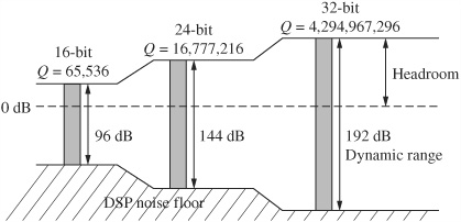
FIGURE 17.18 The dynamic range of fixed-point DSP chips is directly based on their word length. In some applications, double precision increases the effective dynamic range.
The IEEE 752 floating-point standard allows either 32-bit single precision (24-bit mantissa and 8-bit exponent) or double precision (64-bit with a 52-bit mantissa and 11-bit exponent). The latter allows very high-fidelity processing, but is not available on all DSP chips.
DSP Programming
As with all software programming, DSP programming allows the creation of applications with tremendous power and flexibility. The execution of software instructions is accomplished by the DSP chip using audio samples as the input signal. Although the architecture of a DSP chip determines its theoretical processing capabilities, performance is also affected by the structure and diversity of its instruction set.
DSP chips use assembly language programming, which is highly efficient. Higher-level languages (such as C++) are easy to use, document, debug, and are independent of hardware. However, they are less efficient and thus slower to execute, and do not take advantage of specialized chip hardware. Assembly languages are more efficient. They execute faster, require less memory, and take advantage of special hardware functions. However, they are more difficult to program, read, debug, are hardware-dependent, and are labor-intensive.
An assembly language program for a specific DSP chip type is written using the commands in the chip’s instruction set. These instructions take advantage of the chip’s specialized signal processing functions. Generally, there are four types of instructions: arithmetic, program control, memory access and transfer, and input/output. Instructions are programmed with mnemonics that identify the instruction, and reference a data field to be operated upon. Because many DSP chips operate within a host environment, user front-end programs are written in higher-level languages, reserving assembly language programming for the critical audio processing tasks.
An operation that is central to DSP programming is the multiply-accumulate command, often called MAC. Many algorithms call for two numbers to be multiplied, and the result summed with a previous operation. DSP chips feature a multiply-accumulate command that moves two numbers into position, multiplies them together, and accumulates the result, with rounding, all in one operation. To perform this efficiently, the arithmetic unit contains a multiplier–accumulator combination (see Fig. 17.17). This can calculate one subproduct and simultaneously add a previous subproduct to a sum, in one machine cycle. To accommodate this, DSP chips rely on a hardware-multiplier to execute the multiply-accumulate operation. Operations such as sum of products and iterative operations can be performed efficiently.
In most cases, the success of a DSP application depends on the talents of the human programmer. Software development costs are usually much greater than the hardware itself. In many cases, manufacturers supply libraries of functions such as FFTs, filters, and windows that are common to many DSP applications. To assist the development process, various software development tools are employed. A text editor is used to write and modify assembly language source code. An assembler program translates assembly language source code into object code. A compiler translates programs written in higher-level languages into object code. A linker combines assembled and compiled object programs with library routines and creates executable object code. The assembler and compiler use the special processing features of the DSP chip wherever possible. A simulator is used to emulate code on a host computer before running it on DSP hardware. A debugger is used to perform low-level debugging of DSP programs. In addition, DSP operating systems are available, providing programming environments similar to those used by general purpose processors.
Filter Programming
DSP chips can perform many signal processing tasks, but digital filtering is central to many applications. As an example of assembly language programming, consider the FIR transversal filter shown in Fig. 17.19A. It can be described with this difference equation:
y(n) = x(n − 4)h(4) + x(n − 3)h(3) + x(n − 2)h(2) + x(n − 1)h(1) + x(n)h(0)
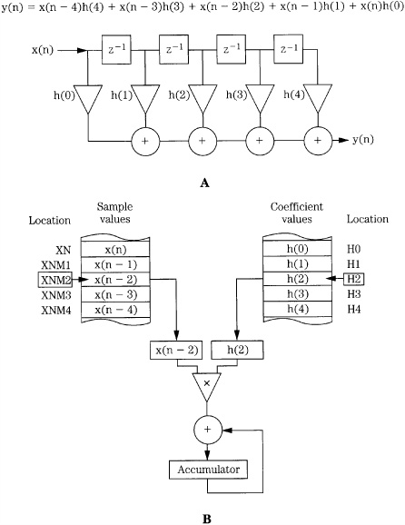
FIGURE 17.19 A five-coefficient FIR filter can be realized with assembly language code authored for a commercial DSP chip. A. Structure of the FIR filter. B. Audio sample and filter coefficient values stored in memory are multiplied and accumulated to form the output samples.
The five input audio sample values, five coefficients describing the impulse response at five sample times, and the output audio sample value will be stored in memory locations; data value x(n) will be stored in memory location XN; x(n - 1) in XNM1; y(n) in YN; h(0) in H0, and so on. The running total will be stored in the accumulator, as shown in Fig. 17.19B. In this case, intermediate calculations are held in the T register.
Texas Instruments Code
The code to execute this five-coefficient FIR filter on a Texas Instruments TMS320xxx chip is shown below:
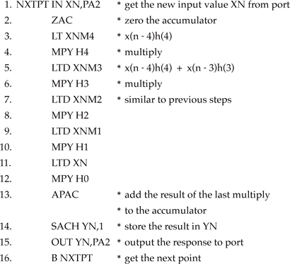
Of particular interest is the LTD instruction that loads a value into a register, adds the result of the last multiply to the accumulator, and shifts the value to the next higher memory address.
Line 1 moves an input data word from an I/O port to memory location XN. Line 2 zeros the accumulator. Line 3 loads the past value XNM4 into the T register. Line 4 multiplies the contents of the T register with the coefficient in H4. Lines 5 and 6 multiply XNM3 and H3, and the LTD instruction adds the result of the line 4 multiplication to the accumulator. Similarly, the other filter taps are multiplied and accumulated in lines 7 through 12. Line 13 adds the final multiplication to the accumulator, so that the accumulator contains the filtered output value corresponding to the input value from line 1. Line 14 transfers this output to YN. Line 15 transfers location YN to the I/O port. Line 16 returns the program to line 1 where the next input value is received.
When the new input is received, past values are shifted one memory location; XN moves to XNM1, XNM1 to XNM2, XNM2 to XNM3, XNM3 to XNM4, and XNM4 is dropped. Although these shifts could be performed with additional instructions, as noted, the LTD instruction (an example of the power of parallel processing) shifts each value to the next higher address after it is transferred to the T register. After line 11, the data values are ready for the next pass. Other program sections not shown would set up I/O ports, synchronize I/O with the sampling rate of external hardware, and store filter coefficients. This particular filter example uses straight-line code with separate steps for each filter tap. It is very fast for short filters, but longer filters would be more efficiently performed with looped algorithms. The decision of which is more efficient for a given filter is not always obvious.
Motorola Code
The Motorola DSP56xxx family of processors are widely used to perform DSP operations such as filtering. Efficiency stems from the DSP chip’s ability to perform multiply-accumulate operations while simultaneously loading registers for the next multiply-accumulate operation. Further, hardware do-loops and repeat instructions allow repetition of the multiply-accumulate operation.
To illustrate programming approaches, the difference equation for the five-coefficient FIR filter in the previous example (see Fig. 17.19) will be realized twice, using code written by Thomas Zudock. First, as in the previous example, the filter is implemented with the restriction that each operation must be executed independently in a straight-line fashion. Second, the filter is implemented using parallel move and looping capabilities to maximize efficiency as well as minimize code size.
First, some background on the DSP56xxx family syntax and architecture. The DSP56xxx has three parallel memories, x, y, and p. Typically, the x and y memories are used to hold data, and the p memory holds the program that performs the processing. The symbols r0 and r5 are address registers. They can be used as pointers to read or write values into any of the three memories. For example, the instruction “move x:(r0) + ,x0” reads the value stored at the memory location pointed to by r0 in x memory into the x0 data register, then increments the r0 address register pointer to the data to be accessed. The x0 and y0 symbols are data registers, typically used to hold the next data that is ready for a mathematical operation. The accumulator is denoted by a; it is the destination for mathematical operations. The instruction “mac x0,y0,a” is an example of the multiply-accumulate operation; the data registers x0 and y0 are multiplied and then summed with the value held in accumulator a.
In a straight-line coded algorithm implementing the FIR example, each step is executed independently. At the start, x0 is already loaded with a new sample, r0 points to the location in x memory to save that sample, and r5 points to the location in memory where h(0) is located. The FIR straight-line code is:
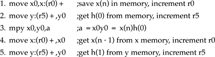
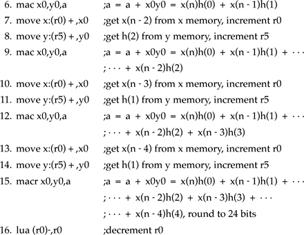
In line 1, the just-acquired sample x(n), located in x0, is moved into the x memory location pointed to by r0, and r0 is advanced to point to the next memory location, the previous sample. In line 2, the filter coefficient in the y memory pointed to by r5, h(0), is read into data register y0, and r5 is incremented to point to the next filter coefficient, h(1). In line 3, x(n) and h(0) are multiplied and the result is stored in accumulator a. The initial conditions of the algorithm, and the status of the algorithm after line 3 can be described as:
Initial Status: x0 = x(n) the sample just acquired
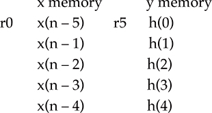
After line 3: a = x0y0 = x(n)h(0)
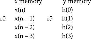
![]()
The remainder of the program continues similarly, with the next data value loaded into x0 and the next filter coefficient loaded into y0 to be multiplied and added to accumulator a. After line 16, the difference equation has been fully evaluated and the filtered output sample is in accumulator a. This status can be described as:
After line 15:
a = x0y0 = x(n)h(0) + x(n − 1)h(1) + x(n − 2)h(2) + x(n − 3)h(3) + x(n − 4)h(4)
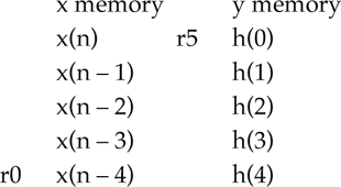
After the next input sample is acquired, the same process will be executed to generate the next output sample. Address registers r0 and r5 have wrapped around to point to the needed data and filter coefficients. The registers are set up for modulo addressing with a modulus of five (because there are five filter taps). Instead of continuing to higher memory, they wrap around in a circular fashion when incremented or decremented to repeat the process again.
Although this code evaluates the difference equation, the DSP architecture has not been used optimally; this filter can be written much more efficiently. Values stored in x and y memory can be accessed simultaneously with execution of one instruction. While values are being multiplied and accumulated, the next data value and filter coefficient can be simultaneously loaded in anticipation of the next calculation. Additionally, a hardware loop counter allows repetition of this operation, easing implementation of long difference equations. The operations needed to realize the same filter can be implemented with fewer instructions and in less time, as shown below. The FIR filter coded using parallel moves and looping is:
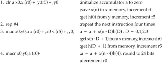
The parallel move and looping implementation is clearly more compact. The number of comments needed to describe each line of code is indicative of the power in each line. However, the code can be confusing because of its consolidation. As programmers become more experienced, use of parallel moves becomes familiar. Many programmers view the DSP56xxx code as having three execution flows: the instruction execution, x memory accesses, and y memory accesses.
The Motorola DSP563xx core uses code that is compatible with the DSP56xxx family of processors. For example, the DSP56367 is a 24-bit fixed-point, 150 MIPS DSP chip. It is used to process multichannel decoding standards such as Dolby Digital and DTS. It can simultaneously perform other audio processing such as bass management, sound-field effects, equalization, and ProLogic II.
Analog Devices SHARC Code
Digital audio processing is computation-intensive, requiring processing and movement of large quantities of data. Digital signal processors are specially designed to efficiently perform the audio and communication chores. They have a high degree of parallelism to perform simultaneous tasks (such as processing multichannel audio files), and balance performance with I/O requirements to avoid bottlenecks. In short, such processors are optimized for audio processing tasks.
The architecture used in the ADSP-2116x SHARC family of DSP chips is an example of how audio computation can be optimized in hardware. As noted, intermediate DSP calculations require higher precision than the audio signal resolution; for example, 16-bit processing is certainly inadequate for a 16-bit audio signal, unless double-precision processing is used. Errors from rounding and truncation, overflow, coefficient quantization, and limit cycles would all degrade signal quality at the D/A converter. Several aspects of the ADSP-2116x SHARC architecture are designed to preserve a large signal dynamic range. In particular, it aims to provide processing precision that will not introduce artifacts into a 20- or 24-bit audio signal.
This architecture performs native 32-bit fixed-point, 32-bit IEEE 754-1985 floating-point, and 40-bit extended precision floating-point computation, with 32-bit filter coefficients. Algorithms can be switched between fixed- and floating-point modes in a single instruction cycle. This alleviates the need for double-precision mathematics and the associated computational overhead. The chip has two DSP processing elements onboard, designated PEX and PEY, each containing an arithmetic logic unit, multiplier, barrel shifter, and register file. The chip also has circular buffer support for up to 32 concurrent delay lines. To help prevent overflow in intermediate calculations, the chip has four 80-bit fixed-point accumulators; two 32-bit values can be multiplied with a 16-bit guard band. Also, multiple link ports allow data to move between multiple processors.
Dual processing units allow single-instruction multiple-data (SIMD) parallel operation in which the same instruction can be executed concurrently in each processing element with different data in each element. Code is optimized because each instruction does double duty. For example, in stereo processing, the left and right channels could be handled separately in each processing element. Alternatively, a complex block calculation such as an FFT can be evenly divided between both processing elements. The code example shown below computes the simultaneous computation of two FIR filters:
/* initialize pointers */
b0 = DELAYLINE;
I0 = @ DELAYLINE;
b8 = COEFADR;
I8 = @ COEFADR;
m1 = -2; m0=2; m8=2;
/* Circular Buffer Enable, SIMD MODE Enable */
bit set MODE1 CBUFEN I PEYEN;
nop;
f0 = dm(samples);
dm(i0,m0) = f0, f4 = pm(i8,m8);
f8 = f0*f4, f0 = dm(i0,m0), f4 = pm(i8,m8);
f12 = f0*f4, f0 = dm(i0,m0), f4 = pm(i8,m8);
Icntr = (TAPS-3), do macs until Ice;
/*FIR loop*/
macs: f12 = f0*f4, f8 = f8 + f12, f0 = dm(i0,m0), f4 = pm(i8,m8);
f12 = f0*f4, f8 = f8 + f12, f0 = dm(i0,m1);
f8 = f8 + f12;
To execute two filters simultaneously in this example, audio samples are interleaved in 64-bit data memory and coefficients are interleaved in 64-bit program memory, with 32 bits for each of the processing elements in upper and lower memory. A single-cycle, multiply-accumulate, dual-memory fetch instruction is used. It executes a single tap of each filter computing the running average while fetching the next sample and next coefficient.
Specialized DSP Applications
Beyond digital filtering, DSP is used in a wide variety of audio applications. For example, building on the basic operations of multiplication and delay, applications such as chorusing and phasing can be developed. Reverberation perhaps epitomizes the degree of time manipulation possible in the digital domain. It is possible to synthesize reverberation to both simulate natural acoustical environments, and create acoustical environments that could not physically exist. Digital mixing consoles embody many types of DSP processing in one consolidated control set. The power of digital signal processing also is apparent in the algorithms used to remove noise from audio signals.
Digital Delay Effects
A delay block is a simple storage unit, such as a memory location. A sample is placed in memory, stored, then recalled some time later and output. A delay unit can be described by the equation: y(n) = x(n - m) where m is the delay in samples. Generally, when the delay is small, the frequency response of the signal is altered; when the delay is longer, an echo results. Just as in filtering, a simple delay can be used to create sophisticated effects. For example, Fig. 17.20A shows an echo circuit using a delay block. Delay mT is of duration m samples, and samples are multiplied by a gain coefficient (a scaling factor) less than unity. If the delay time is set between 10 ms and 50 ms, an echo results; with shorter fixed delays, a comb filter response results, as shown in Fig. 17.20B. Peaks and dips are equally spaced through the frequency response, from 0 Hz to the Nyquist frequency. The number of peaks depends on the delay time; the longer the delay, the greater the number of peaks.
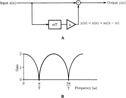
FIGURE 17.20 A delay block can be used to create an echo circuit. A. The circuit contains an mT delay and gain stage. B. With shorter delay times, a comb filter response will result. (Bloom, 1985; Berkhout and Eggermont, 1985)
If the delay time of the circuit in Fig. 17.20A is slowly varied between 0 ms and 10 ms, the time-varying comb filter creates a flanging effect. If the time delay is varied between 10 ms and 25 ms, a doubling effect is achieved, giving the impression of an accompanying voice. A chorus effect is provided when the signal is directed through several such blocks, with different delay variations.
A comb filter can be either recursive or nonrecursive. It cascades a series of delay elements, creating a new response. Mathematically, we see that a nonrecursive comb filter, such as the one described above, can be designed by adding the input sample to the same sample delayed: y(n) = x(n) + ax(n - m) where m is the delay time in samples. A recursive comb filter creates a delay with feedback. The delayed signal is attenuated and fed back into the delay: y(n) = ax(n) + by(n - m). This yields a response as shown in Fig. 17.21. The number of peaks depends on the duration of the delay; the longer the delay, the greater the number of peaks.
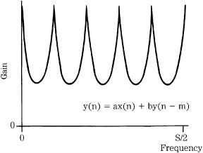
FIGURE 17.21 A recursive comb filter creates a delay with feedback, yielding a toothed frequency response.
An all-pass filter is one that has a flat frequency response from 0 Hz to the Nyquist frequency. However, its phase response causes different frequencies to be delayed by different amounts. An all-pass filter can be described as: y(n) = -ax(n) + x(n - 1) + by(n - 1).
If the delay in the above circuits is replaced by a digital all-pass filter or a cascade of all-pass filters, a phasing effect is achieved: y(n) = -ax(n) + x(n - m) + by(n - m). The effect becomes more pronounced as the delay increases. The system exhibits nonuniformly spaced notches in its frequency response, varying independently in time.
Digital Reverberation
Reflections are characterized by delay, relative loudness, and frequency response. For example, in room acoustics, delay is determined by the size of the room, and loudness and frequency response are determined by the reflectivity of the boundary surfaces and surface construction. Digital reverberation is ideally suited to manipulate these parameters of an audio signal, to create acoustical environments. Because reverberation is composed of a large number of physical sound paths, a digital reverberation circuit must similarly process many data elements.
Both reverberation and delay lines are fundamentally short-memory devices. A pure delay accepts an input signal and reproduces it later, possibly a number of times at various intervals. With reverberation, the signal is mixed repetitively with itself during storage at continually shorter intervals and decreasing amplitudes. In a delay line, the processor counts through RAM addresses sequentially, returning to the first address after the last has been reached. A write instruction is issued at each address, and the sampled input signal is routed to RAM. In this way, audio information is continually stored in RAM for a period of time until it is displaced by new information. During the time between write operations, multiple read instructions can be issued sequentially with different addresses. By adjusting the numerical differences, the delay times for the different signals can be determined.
In digital reverberation, the stored information must be read out a number of times, and multiplied by factors less than unity. The result is added together to produce the effect of superposition of reflections with decreasing intensity. The reverberation process can be represented as a feedback system with a delay unit, multiplier, and summer. The processing program in a reverberation unit corresponds to a series and parallel combination of many such feedback systems (for example, 20 or more). Recursive configurations are often used. The single-zero unit reverberator shown in Fig. 17.22A generates an exponentially decreasing impulse response when the gain block is less than unity. It functions as a comb filter with peaks spaced by the reciprocal of the delay time. The echoes are spaced by the delay time, and the reverberation time can be given as: RT = 3T/log10(a) where T is the time delay and a is the coefficient. Sections can be cascaded to yield more densely spaced echoes; however, resonances and attenuations can result. Overall, it is not satisfactory as a reverberation device.
Alternatively, a reverberation section can be designed from an all-pass filter. The filter shown in Fig. 17.22B yields an all-pass response by adding part of the unreverberated signal to the output. Total gain through the section is unity. In this section, frequencies that are not near a resonance and thus not strongly reverberated are not attenuated. Thus, they can be reverberated by a following section. Other types of configurations are possible; for example, Fig. 17.22C shows an all-pole section of a reverberation circuit which can be described as: y(n) = -ax(n) + x(n - m) + ay(n - m).
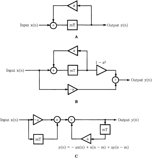
FIGURE 17.22 Reverberation algorithms can be constructed from recursive configurations. A. A simple reverberation circuit derived from a comb filter. B. A reverberation circuit derived from an all-pass filter. C. A reverberation circuit constructed from an all-pole section. (Blesser et al., 1975)
The spacing between the equally spaced peaks in the frequency response is determined by the delay time, and their amplitude is set by the scaling coefficients. One reverberation algorithm devised by Manfred Schroeder uses four reverberant comb filters in parallel followed by two reverberant all-pass filters in series, as shown in Fig. 17.23. The four comb filters, with time delays ranging from 30 ms to 45 ms, provide sustained reverberation, and the all-pass networks with shorter delay times contribute to reverberation density. The combination of section types provides a relatively smooth frequency response, and permits adjustable reverberation times. Commercial implementations are often based on similar methods, with the exact algorithm held in secrecy.
Digital Mixing Consoles
The design of a digital mixing console is quite complex. The device is, in effect, a vast digital signal processor, requiring perhaps 109 instructions per second. Although many of the obstacles present in analog technology are absent in a digital implementation, seemingly trivial exercises in signal processing might require sophisticated digital circuits. In addition, the task of real-time computation of digital signal processing presents problems unique to digital architecture. The digital manifestation of audio components requires a rethinking of analog architectures and originality in the use of digital techniques.
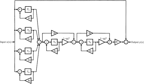
FIGURE 17.23 Practical reverberation algorithms yielding natural sound contain a combination of reverberation sections. (Schroeder, 1962)
A digital console avoids numerous problems encountered by its analog counterpart, but its simple task of providing the three basic functions of attenuating, mixing, and signal selection and routing entails greater design complexity. The problem is augmented by the requirement that all operations must be interfaced to the user’s analog world. A virtual mixer is much easier to design than one with potentiometers and other physical comforts. In either case, a digital console’s software-defined processing promotes flexibility.
The processing tasks of a digital console follow those of any DSP system. The first fundamental task of a mixing console is gain control. In analog, this is realized with only a potentiometer. However, a digital preamplifier requires a potentiometer, an A/D converter to convert the analog position information of the variable resistor into digital form, and a multiplier to adjust the value of the digital audio data, as shown in Fig. 17.24A. The mixing console’s second task, mixing, can be accomplished in the analog domain with several resistors and an operational amplifier. In a digital realization, this task requires a multiplexer and accumulator, as shown in Fig. 17.24B. The third task, signal selection and routing, is accomplished in analog with a multipole switch, but digital technology requires a demultiplexer and encoding circuit to read the desired selection, as shown in Fig. 17.24C. All processing steps must be accomplished on each audio sample in each channel in real time, that is, within the span of one sample period (for example, 10.4 μs at a 96-kHz sampling frequency). For real-time applications such as broadcasting and live sound, throughput latency must be kept to a minimum.
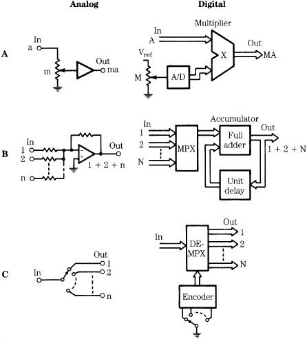
FIGURE 17.24 The three primary functions in signal processing can be realized in both analog and digital forms. A. Attenuating. B. Mixing. C. Selecting. (Sakamoto et al., 1982)
Any console must provide equalization faculties such as lowpass, highpass, and shelving filters. These can be designed using a variety of techniques, such as a cascade of biquadratic sections, a type of digital filter architecture. The fast processing speeds and necessity for long word length place great demands on the system. On the other hand, filter coefficients are readily stored in ROM, and no more than a few thousand characteristics are typically required for most applications.
Because the physical controls of a digital console are simply remote controls for the processing circuits, no audio signal passes through the console surface. It is thus possible to offer assignable functions. Although the surface might emulate a conventional analog console with parallel controls, a set of fewer assignable controls can be used as a basic control set to view and control the mix elements. For example, after physical controls are used to record and equalize basic tracks, they can be assigned to virtual strips that are not assigned to physical controls, then individually reassigned back to physical controls as needed. In other words, the relationship between the number of physical channel strips and the number of console inputs and outputs is flexible. The console can provide a central control section that provides access to all of the assignable functions currently requested for a particular signal path.
Particular processing functions can be assigned to a channel, inserted in the signal path, and controlled from that channel’s strip or elsewhere. Physical controls on a channel strip can provide different functions, with displays that reflect the value of the selected function. A set of controls might provide equalization, or auxiliary sends. In another example, one channel strip might be assigned to a monaural, or stereo channel. As a session progresses from tracking to mix-down, the console can gradually be reconfigured, for example, adding more sends, then later creating subgroups. There is no need to limit controls to the equivalent fixed analog circuit parameters. Thus, rotary knobs, for example, might have no end stops and can be programmed for various functions or resolution. For example, equalization might be accomplished in fractions of decibels, with selected values displayed.
Console setup can be accomplished via an alphanumeric keyboard, and particular configurations can be saved in memory, or preprogrammed in presets for rapid changeover in a real-time application. Flexibility would be more of a curse than a blessing if the operator were required to build a software console from scratch each time. Therefore, using the concept of a “soft” signal path, multiple console preset configurations may be available: track laying, mix-down, return to previous setting, and a fail-safe minimum mode.
A video display might show graphical representations of console signal blocks as well as their order in the signal path. This is useful when default settings of delay, filter, equalization, dynamics, and fader are varied. In addition, each path can be named, and its fader assignment shown, as well as its mute group, solo status, phase reverse, phantom power on/off, time delay, and other parameters.
Loudspeaker Correction
Loudspeakers are far from perfect. Their nonuniform frequency response, limited dynamic range, frequency-dependent directivity, and phase nonlinearity all degrade the reproduced audio signal. In addition, a listening room reinforces and cancels selected frequencies in different room locations, and contributes surface reflections, superimposing its own sonic signature on that of the audio signal. Using DSP, correction signals can be applied to the audio signal. Because the corrections are opposite to the errors in the acoustically reproduced signal, they theoretically cancel them.
Loudspeakers can be measured as they leave the assembly line, and deviations such as nonuniform frequency response and phase nonlinearity can be corrected by DSP processing. Because small variations exist from one loudspeaker to the next, the DSP program’s coefficients can be optimized for each loudspeaker. Moreover, certain loudspeaker/room problems can be addressed. For example, floor-standing loudspeakers can have predetermined relationships between the drivers, the cabinet, and the reflecting floor surface. The path-length difference between the direct and reflected sound creates a comb-filtered frequency response that can be corrected using DSP processing.
A dynamic approach can be used in an adaptive loudspeaker/room correction system, in which the loudspeakers generate audio signals to correct the unwanted signals reflected from the room. Using DSP chips and embedded software programs, low-frequency phase delay, amplitude and phase errors in the audio band, and floor reflections can all be compensated for. Room acoustical correction starts with room analysis, performed on-site. Using a test signal, the loudspeaker/room characteristics are collected by an instrumentation microphone placed at the listening position, and processed by a program that generates room-specific coefficients. The result is a smart loudspeaker that compensates for its own deficiencies, as well as anomalies introduced according to its placement in a particular room.
Noise Removal
Digital signal processing can be used to improve the quality of previously recorded material or restore a signal to a previous state, for example, by removing noise. With DSP it is possible to characterize a noise signal and minimize its effect without affecting a music signal. For example, DSP can be used to reduce or remove noises such as clicks, pops, hum, tape hiss, and surface noise from an old recording. In addition, using methods borrowed from the field of artificial intelligence, signal lost due to tape dropouts can be synthesized with great accuracy. Typically, noise removal is divided into two tasks, detection and elimination of impulsive noise such as clicks, and background noise reduction.
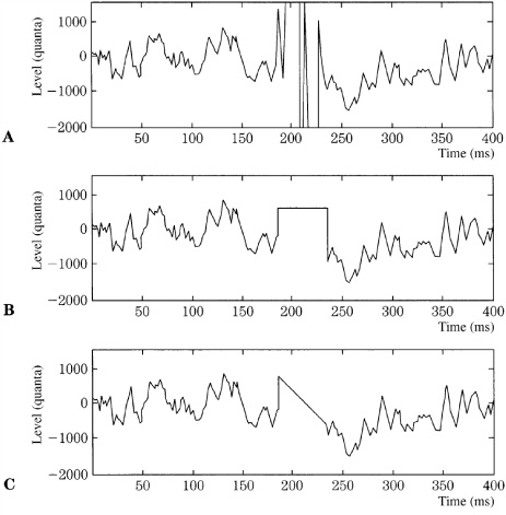
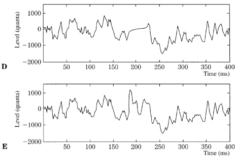
FIGURE 17.25 Examples showing how interpolation can be used to overcome an impulsive click. Higher-order interpolation can synthesize an essentially inaudible bridge. A. Original sample with click. B. Sample and hold with highpass click detection. C. Straight-line interpolation. D. Low-order interpolation. E. High-order interpolation.
Interactive graphical displays can be used to locate impulsive disturbances. A de-clicking program analyzes frequency and amplitude information around the click, and synthesizes a signal over the area of the click. Importantly, the exact duration of the performance is preserved. For example, Fig. 17.25 shows a music segment with a click and the success of various de-clicking methods. A basic sample-and-hold function produces a plateau that is preferable to a loud click. With linear interpolation the click is replaced by a straight line connecting valid samples. Interpolation can be improved by using a signal model to measure local signal characteristics (a few samples). Interpolation can be further improved by increasing the number of samples used in the model (hundreds of samples). Automatic de-clicking algorithms similarly perform interpolation over defects, but first must differentiate between unwanted clicks, and transient music information. Isolated clicks will exhibit short rise and decay times between amplitude extremes but a series of interrelated clicks can be more difficult to identify. When more than one copy of a recording is available (or when the same signal is recorded on two sides of a groove), uncorrelated errors are more easily identified. However, different recordings must be precisely time-aligned.
A background noise-removal process can begin by dividing the audio spectrum into frequency bands, then performing an analysis to determine content. The spectral composition of surface noise and hiss is determined and this fingerprint is used to develop an inverse function to remove the noise. Ideally, the fingerprint data is taken from a silent portion of the recording, perhaps during a pause. Because there is no music signal, the noise can be more accurately analyzed. Alternatively, samples can be taken from an area of low-amplitude music, and a noise template applied.
For removal of steady-state artifacts, the audio signal is considered in small sections. The energy in each frequency band is compared to that in the noise fingerprints and the system determines what action to take in each frequency band. For example, at a particular point in the program, music can dominate in a lower spectrum and the system can pass the signal in that band unprocessed, but hiss dominating at a higher frequency might trigger processing in that band. In many cases, some original noise is retained, because the result is generally more natural sounding. In some algorithms, a clean audio signal is estimated and then analyzed to create a masking curve. Only noise that is not masked by the curve is subjected to noise removal; this minimizes introduction of artifacts or damage to the audio signal.
Hiss from a noisy analog recording, wind noise from an outdoor recording, hum from an air conditioner, even the noise obscuring speech in a downed aircraft’s flight recorder can all be reduced in a recording. In short, a processed recording can sound better than the original master recording. On the other hand, as with most technology, noise removal processing requires expertise in its application, and improper use degrades a recording. One question is the degree to which processing is applied. A 10 to 15% reduction in noise level can make the difference between an acceptable recording, and an unpleasantly noisy one. Additional noise removal can be problematic, even if it is only psychoacoustical tricks that make us think it is the audio signal that is being affected.
Thomas Stockham’s experiments on recordings made by Enrico Caruso in 1906 resulted in releases of digitally restored material in which those acoustical recordings were analyzed and processed with a blind deconvolution method, so-called because the nature of the signals operated upon cannot be precisely defined. In this case, the effect of an unknown filter on an unknown signal was removed by observing the effect of the filtering. By averaging a large number of signals, constant signals could be identified relative to dynamic signals. In this way, the strong resonances of the horn used to make these acoustical recordings, and other mechanical noise, were estimated and removed from the recording by applying an inverse function, leaving a restored audio signal.
In essence, the acoustical recording process was viewed as a filter. The music and the impulse response of the recording system were convolved. From this analysis of the playback signal, the original performance’s spectrum was multiplied by that of the recording apparatus, and then inverse Fourier transformed to yield the signal actually present on the historic recordings. Correspondingly, the undesirable effects of the recording process were removed from the true spectrum of the performance. The computation of a correction filter using FFT methods was not a trivial task. A long-term average spectrum was needed for both the recording to be restored, and for a model, higher-fidelity recording. In Stockham’s work, a 1-minute selection of music required about 2500 FFTs for complete analysis. The difference between the averaged spectra of the old and new recordings was computed, and became the spectrum of the restoration filter. Restoration required multiplying segments of the recording’s spectrum by the restoration spectrum and performing inverse FFTs, or by direct convolution using a filter impulse response obtained through inverse FFT.
Blind deconvolution uses techniques devised by Alan Oppenheim, known as generalized linearity or homomorphic signal processing. This class of signal processing is nonlinear, but is based upon a generalization of linear techniques. Convolved or multiplied signals are nonlinearly processed to yield additive representations, which in turn are processed with linear filters and returned via an inverse nonlinear operation to their original domain. These and other more advanced digital-signal processing topics are discussed in detail in other texts.