CHAPTER 5
Error Correction

The advent of digital audio changed audio engineering forever and introduced entirely new techniques. Error correction was perhaps the most revolutionary new technique of them all. With analog audio, there is no opportunity for error correction. If the conveyed waveform is disrupted or distorted, then the waveform is usually irrevocably damaged. It is impossible to exactly reconstruct an infinitely variable waveform. With digital audio, the nature of binary data lends itself to recovery in the event of damage. When a bit is diagnosed as incorrect, it is easy to invert it. To permit this, when audio data is stored or transmitted, it can be specially coded and accompanied by redundancy. This enables the reproduced data to be checked for errors. When an error is detected, further processing can be performed to absolutely correct the error. In the worst case, errors can be concealed by synthesizing new data. In either case, error correction makes digital data transmission and storage much more robust and indeed makes the systems more efficient. Strong error-correction techniques allow a channel’s signal-to-noise ratio to be reduced; thus, for example, permitting lower power levels for digital broadcasting. Similarly, error correction relaxes the manufacturing tolerances for mass media such as CD, DVD, and Blu-ray.

However, error correction is more than a fortuitous opportunity; it is also an obligation. Because of high data densities in audio storage media, a petty defect in the manufactured media or a particle of dust can obliterate hundreds or thousands of bits. Compared to absolute numerical data stored digitally, where a bad bit might mean the difference between adding or subtracting figures from a bank account, digital audio data is relatively forgiving of errors; enjoyment of music is not necessarily ruined because of occasional flaws in the output waveform. However, even so, error correction is mandatory for a digital audio system because uncorrected audible errors can easily occur because of the relatively harsh environment to which most audio media are subjected.

Error correction for digital audio is thus an opportunity to preserve data integrity, an opportunity not available with analog audio, and it is absolutely necessary to ensure the success of digital audio storage, because errors surely occur. With proper design, digital audio systems such as CD, DVD, and Blu-ray can approach the computer industry standard, which specifies an error rate of 10⁻¹², that is, less than one uncorrectable error in 10¹² (one trillion) bits. However, less stringent error performance is adequate for most audio applications. Without such protection, digital audio recording would not be viable. Indeed, the evolution of digital audio technology can be measured by the prerequisite advances in error correction.

Sources of Errors

Degradation can occur at every stage of the digital audio recording chain. Quantization error, converter nonlinearity, and jitter can all limit system performance. High-quality components, careful circuit design, and strict manufacturing procedures minimize these degradations. For example, a high-quality analog-to-digital (A/D) converter can exhibit satisfactory low-level linearity, and phase-locked loops can overcome jitter.

The science of error correction mainly attends to stored and transmitted data, because it is the errors presented by those environments that are most severe and least subject to control. For example, optical media can be affected by pit asymmetry, bubbles or defects in substrate, and coating defects. Likewise, for example, transmitted data is subject to errors caused by interfering signals and atmospheric conditions.

Barring design defects or a malfunctioning device, the most severe types of errors occur in the recording or transmission signal chains. Such errors result in corrupted data, and hence a defective audio signal. The most significant cause of errors in digital media is dropouts, essentially a defect in the medium that causes a momentary drop in signal strength. Dropouts can occur in any optical disc and can be traced to two causes: a manufactured defect in the medium or a defect introduced during use. Transmitted signals are vulnerable to disturbances from many types of human-made or natural interference. The effects of noise, multipath interference, crosstalk, weak signal strength, and fading are familiar to all cell phone users.

Defects in storage media or disruptions during transmission can cause signal transitions that are misrepresented as erroneous data. The severity of the error depends on the nature of the error. A single bad bit can be easily corrected, but a string of bad bits may be uncorrectable. An error in the least significant bit of a PCM word may pass unnoticed, but an error in the most significant bit may create a drastic change in amplitude. Usually, a severe error results in a momentary increase in noise or distortion or a muted signal. In the worst case, a loss of data or invalid data can provoke a click or pop, as the digital-to-analog converter’s output jumps to a new amplitude while accepting invalid data.

Errors occur in several modes; thus, classifications have been developed to better identify them. Errors that have no relation to each other are called random-bit errors. These random-bit errors occur singly and are generally easily corrected. A burst error is a large error, disrupting perhaps thousands of bits, and requires more sophisticated correction. An important characteristic of any error-correction system is the burst length, that is, the maximum number of adjacent erroneous bits that can be corrected. Both random and burst errors can occur within a single medium; therefore, an error-correction system must be designed to correct both error types simultaneously.

In addition, because the nature of errors depends on the medium, error-correction techniques must be optimized for the application at hand. Thus, storage media errors, wired and wireless transmission errors must be considered separately. Finally, error-correction design is influenced by the kind of modulation code used to convey the data.

Optical discs can suffer from dropouts resulting from various manufacturing and handling problems. When a master disc is manufactured, an incorrect intensity of laser light, incorrect developing time, or a defect in the photoresist can create badly formed pits. Dust or scratches incurred during the plating or pressing processes, or pinholes or other defects in the discs’ reflective coating can all create dropouts. Stringent manufacturing conditions and quality control can prevent many of these dropouts from leaving the factory. Optical discs become dirty or damaged with use. Dust, dirt, and oil can be wiped clean; however, scratches might interfere with the pickup’s ability to read data. Although physically small to bulky humans, foreign objects such as those shown in Fig. 5.1 are large when it is considered that the recorded bit size can be much smaller than 1 μm (micrometer). When cleaning optical media such as a Compact Disc, a clean, soft cloth should be used to wipe the disc radially, that is, across the width of the disc and not around its circumference. Any scratches that result will be perpendicular to tracks and thus easier to correct, but a single scratch along one track could be impossible to correct because of the sustained consecutive loss of data.

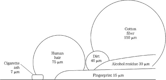
FIGURE 5.1 Small physical objects are large in the context of a 1-μm recorded bit size.

Hard-disk magnetic media are enclosed in a sealed, protective canister and are mainly immune to dust and dirt contamination. Moreover, bad sectors are marked and not used for recording; only minimal error correction is needed.

A number of factors conspire to degrade the quality of wired data channels including limited bandwidth and intersymbol interference, attenuation, noise, ringing, reflection, and substandard cables and connectors. For example, as data travels down a length of cable, the cable acts as a low pass filter, reducing bandwidth and adding group delay. A square-wave signal will show a gradual rise and fall time, and if the data rate is too high, the signal might not reach its full logical 1 and 0 levels. In other words, the level actually representing one bit can partly depend on the level of the previous bit; this is intersymbol interference. Similarly, interference can be caused by signal reflection, echoes from the terminating circuits that can reinforce, or cancel signal levels. Reflections can be caused by impedance mismatches between cables and terminating circuits. Other error sources include external low-frequency noise that can shift data transitions, causing jitter. Radio-frequency (RF) interference must be prevented with proper shielding and grounding. Fiber-optic cables are largely immune to radio-frequency interference and other problems that plague copper cables. The quality of a digital signal can be evaluated from its eye pattern, as discussed in Chap. 4.

Cellular telephones, digital radio, and other audio technologies using wireless transmission and reception are subject to numerous error conditions. These systems use radio waves traveling through air for communication, and these signals may be attenuated or otherwise unreliable, resulting in poor reception, dropped calls, and dead zones. Many types of electronic devices emit unwanted electromagnetic signals which can interfere with wireless communications. Adjacent-channel interference is impairment at one frequency caused by a signal on a nearby channel frequency. Co-channel interference is created by other transmitters using the same channel frequency, for example, in nearby cells. Radio signals can be disrupted by multipath interference created when signals are reflected by a large surface such as a nearby building. Signal strength is affected by location distance or placement of antennas in cellular network architectures, and low network density. Weather conditions as well as solar flares and sunspots can affect signal strength and quality. Signal strength can also be reduced by many kinds of obstructions; this commonly occurs in some buildings, subways, and tunnels, as well as on hilly terrain. Some kinds of obstructions are not intuitively obvious. Excessive foliage can block signals; for example, mobile systems operating in the 800-MHz band are not used in forested areas because pine needles can absorb and obstruct signals at that wavelength.

Quantifying Errors

A number of parameters have been devised to quantify the integrity of data. The bit-error rate (BER) is the number of bits received in error divided by the total number of bits received. For example, a BER of 10⁻⁹ specifies one bit error for 10⁹ (1 billion) bits transmitted. In other words, BER is an error count. An optical disc system, for example, may contain error-correction algorithms able to handle a BER of 10⁻⁵ to 10⁻⁴. The BER specifies the number of errors, but not their distribution. For example, a BER value might be the same for a single large error burst, as for several smaller bursts. Thus the BER is not a good indicator for an otherwise reliable channel subject to burst errors. For example, over 80% of the errors in an optical disc might be burst errors.

Taking a different approach, the block-error rate (BLER) measures the number of blocks or frames of data that have at least one occurrence of uncorrected data. In many cases, BLER is measured as an error count per second, averaged over a 10-second interval. For example, the CD standard specifies that a CD can exhibit a maximum of 220 BLER errors per second, averaged over a 10-second interval. These values do not reflect the literal number of errors, but gauge their relative severity. BLER is discussed in more detail below, in the context of the Reed–Solomon error-correction code. The burst-error length (BERL) counts the number of consecutive blocks in error; it can be specified as a count per second.

Because burst errors can occur intermittently, they are difficult to quantify with a bit-error rate. In some cases, the errored second is measured; this tallies each second of data that contains an error. Errors can be described as the number of errored seconds over a period of time, or the time since the last errored second. As with BLER and BERL, this does not indicate how many bits are in error, but rather counts the occasions of error.

When designing error correction for an audio system, benchmarks such as raw BER and BLER must be accurately estimated because they are critical in determining the extent of error correction needed. If the estimates are too low, the system may suffer from uncorrected errors. On the other hand, if the estimates are too high, too much channel capacity will be given to error-correction redundancy, leaving relatively less capacity for audio data, and thus overall audio fidelity may suffer. No matter how errors are addressed, it is the job of any system to detect and correct errors, keeping uncorrected errors to a minimum.

Objectives of Error Correction

Many types of error correction exist for different applications. Designers must judge the correctability of random and burst errors, redundancy overhead, probability of misdetection, maximum burst error lengths to be corrected or concealed, and the cost of an encoder and decoder. For digital audio, errors that cannot be corrected are concealed. However, sometimes a misdetected error cannot be concealed, and this can result in an audible click in the audio output. Other design objectives are set by the particular application; for example, optical discs are relatively tolerant of fingerprints because the transparent substrate places them out of focus to the optical pickup. Because of the varied nature of errors—some predictable and some unpredictable—error-correction systems ultimately must use various techniques to guard against them.

Many storage or transmission channels will introduce errors in the stored or transmitted data; for accurate recovery, it is thus necessary for the data to include redundancy that overcomes the error. However, redundancy alone will not ensure accuracy of the recovered information; appropriate error-detection and correction coding must be used.

Although a perfect error-correction system is theoretically possible, in which every error is detected and corrected, such a system would create an unreasonably high data overhead because of the amount of redundant data required to accomplish it. Thus, an efficient audio error-correction system aims for a low audible error rate after correction and concealment, while minimizing the amount of redundant data and data processing required for successful operation. An error-correction system comprises three operations:

• Error detection uses redundancy to permit data to be checked for validity.

• Error correction uses redundancy to replace erroneous data with newly calculated valid data.

• In the event of large errors or insufficient data for correction, error concealment techniques substitute approximately correct data for invalid data.

When not even error concealment is possible, digital audio systems can mute the output signal rather than let the output circuitry attempt to decode severely incorrect data, and produce severely incorrect sounds.

Error Detection

All error-detection and correction techniques are based on data redundancy. Data is said to be redundant when it is entirely derived from existing data, and thus conveys no additional information. In general, the greater the likelihood of errors, the greater the redundancy required. All information systems rely heavily on redundancy to achieve reliable communication; for example, spoken and written language contains redundancy. If the garbled lunar message “ONC GIAVT LE?P FOR MHNKIND” is received, the information could be recovered. In fact, Claude Shannon estimated that written English is about 50% redundant. Many messages incorporate both the original message as well as redundancy to help ensure that the message is properly understood.

Redundancy is required for reliable data communication. If a data value alone is generated, transmitted once, and received, there is no absolute way to check its validity at the receiving end. At best, a word that differs radically from its neighbors might be suspect. With digital audio, in which there is usually some correlation from one 48,000th of a second to the next, such an algorithm might be reasonable. However, we could not absolutely detect errors or begin to correct them. Clearly, additional information is required to reliably detect errors in received data. Since the additional information usually originates from the same source as the original data, it is subject to the same error-creating conditions as the data itself. The task of error detection is to properly code transmitted or stored information, so that when data is lost or made invalid, the presence of the error can be detected.

In an effort to detect errors, the original message could simply be repeated. For example, each data word could be transmitted twice. A conflict between repeated words would reveal that one is in error, but it would be impossible to identify the correct word. If each word was repeated three times, probability would suggest that the two in agreement were correct while the differing third was in error. Yet the opposite could be true, or all three words could agree and all be in error. Given enough repetition, the probability of correctly detecting an error would be high; however, the data overhead would be enormous. Also, the increased data load can itself introduce additional errors. More efficient methods are required.

Single-Bit Parity

Practical error detection uses techniques in which redundant data is coded so it can be used to efficiently check for errors. Parity is one such method. One early error-detection method was devised by Islamic mathematicians in the ninth century; it is known as “casting out 9s.” In this technique, numbers are divided by 9, leaving a remainder or residue. Calculations can be checked for errors by comparing residues. For example, the residue of the sum (or product) of two numbers equals the sum (or product) of the residues. It is important to compare residues, and sometimes the residue of a sum or product residue must be taken. If the residues are not equal, it indicates an error has occurred in the calculation, as shown in Fig. 5.2. An insider’s trick makes the method even more efficient; the sum of digits in a number always has the same 9s residue as the number itself. The technique of casting out 9s can be used to cast out any number, and forms the basis for a binary error-detection method called parity.

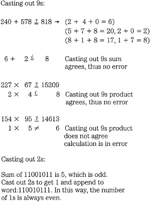
FIGURE 5.2 Casting out of 9s and 2s provides simple error detection.

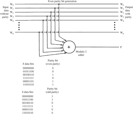
FIGURE 5.3 Parity can be formed through the modulo 2 addition of data bits.

Given a binary number, a residue bit can be formed by casting out 2s. This extra bit is formed when the word is transmitted or stored, and is carried along with the data word. This extra bit, known as a parity bit, permits error detection, but not correction. Rather than cast out 2s, a more efficient algorithm can be used. An even parity bit is formed with two simple rules: if the number of 1s in the data word is even (or zero), the parity bit is a 0; if the number of 1s in the word is odd, the parity bit is a 1. In other words, with even parity, there is always an even number of 1s. To accomplish this, the data bits are added together with modulo 2 addition, as shown in Fig. 5.3. Thus, an 8-bit data word, made into a 9-bit word with an even parity bit, will always have an even number of 1s (or none). This method results in even parity. Alternatively, by forcing an odd number of 1s, odd parity results. Both methods are functionally identical.

At playback, the validity of the received data word is tested using the parity bit; that is, the received data bits are added together to calculate the parity of the received data. If the received parity bit and the calculated parity bit are in conflict, then an error has occurred. This is a single-bit detector with no correction ability. With even parity, for example, the function can determine when an odd number of errors (1, 3, 5, and so on) are present in the received data; an even number of errors will not be detected, as shown in Fig. 5.4. Probability dictates that the error is in the data word, rather than the parity bit itself. However, the reverse could be true.

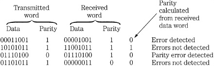
FIGURE 5.4 Examples of single-bit parity error detection.

In many cases, errors tend to occur as burst errors. Thus, many errors could occur within each word and single-bit parity would not provide reliable detection. By itself, a single-bit parity check code is not suitable for error detection in many digital audio storage or transmission systems.

ISBN

For many applications, simple single-bit parity is not sufficiently robust. More sophisticated error detection codes have been devised to make more efficient use of redundancy. One example of coded information is the International Standard Book Number (ISBN) code found on virtually every book published. No two books and no two editions of the same book have the same ISBN. Even soft- and hard-cover editions of a book have different ISBNs.

An ISBN number is more than just a series of numbers. For example, consider the ISBN number, 0-14-044118-2 (the hyphens are extraneous). The first digit (0) is a country code; for example, 0 is for the United States and some other English-speaking countries. The next two digits (14) is a publisher code. The next six digits (044118) is the book title code. The last digit (2) is particularly interesting; it is a check digit. It can be used to verify that the other digits are correct. The check digit is a modulo 11 weighted checksum of the previous digits. In other words, when the digits are added together in modulo 11, the weighted sum must equal the number’s checksum. (To maintain uniform length of 10 digits per ISBN, the Roman numeral X is used to represent the check digit 10.) Given this code, with its checksum, we can check the validity of any ISBN by adding together (modulo 11) the series of weighted digits, and comparing them to the last checksum digit.

Consider an example of the verification of an ISBN code. To form the weighted checksum of a 10-digit number abcdefghij, compute the weighted sum of the numbers by multiplying each digit by its digit position, starting with the leftmost digit:

10a +9b +8c +7d +6e +5f +4g +3h +2i +1j

For the ISBN number 0-14-044118-2, the weighted sum is:

10× 0 + 9× 1 + 8× 4 + 7× 0 + 6× 4 + 5× 4 + 4× 1 + 3× 1 + 2× 8 + 1× 2 = 110

The weighted checksum modulo 11 is found by taking the remainder after dividing by 11:

, with a 0 remainder

The 0 remainder suggests that the ISBN is correct. In this way, ISBNs can be accurately checked for errors. Incidentally, this 10-digit ISBN system (which has the ability to assign 1 billion numbers) is being replaced by a 13-digit ISBN to increase the numbering capacity of the system; it adds a 978 prefix to existing ISBNs, a 979 prefix to new numbers, and retains a checksum. In any case, the use of a weighted checksum compared to the calculated remainder with modulo arithmetic is a powerful way to detect errors. In fact, error-detection codes in general are based on this principle.

Cyclic Redundancy Check Code

The cyclic redundancy check code (CRCC) is an error-detection method used in some audio applications because of its ability to detect burst errors in the recording medium or transmission channel. The CRCC is a cyclic block code that generates a parity check word. The bits of a data word can be added together to form a sum of the bits; this forms a parity check word. For example, in 1011011010, the six binary 1s are added together to form binary 0110 (6 in base 10), and this check word is appended to the data word to form the codeword for transmission or storage. As with single-bit parity, any disagreement between the received checksum and that formed from the received data would indicate with high probability that an error has occurred.

The CRCC works similarly, but with a more sophisticated calculation. Simply stated, each data block is divided by an arbitrary and constant number. The remainder of the division is appended to the stored or transmitted data block. Upon reproduction, division is performed on the received word; a zero remainder is taken to indicate an error-free signal, as shown in Fig. 5.5. A more detailed examination of the encoding and decoding steps in the CRCC algorithm is shown in Fig. 5.6. A message m in a k-bit data block is operated upon to form an n − k bit CRCC detection block, where n is the length of the complete block.

The original k-bit data block is multiplied by X^n−k to shift the data in preparation to appending the check bits. It is then divided by the generation polynomial g to form the quotient q and remainder r. The transmission polynomial v is formed from the original message m and the remainder r; it is thus a multiple of the generation polynomial g. The transmission polynomial v is then transmitted or stored. The received data u undergoes error detection by calculating a syndrome, in the sense that an error is sign of malfunction or disease. Specifically, the operation creates a syndrome c with modulo 2 addition of received parity bits and parity that is newly calculated from the received message. A zero syndrome shows an error-free condition. A nonzero syndrome denotes an error.

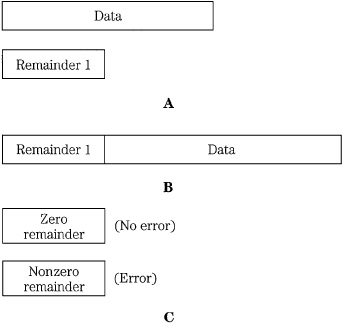
FIGURE 5.5 CRCC in simplified form showing the generation of the remainder. A. Original block of data is divided to produce a remainder. The quotient is discarded. B. The remainder is appended to the data word and both words are transmitted or stored. C. The received data is again divided to produce a remainder, used to check for errors.

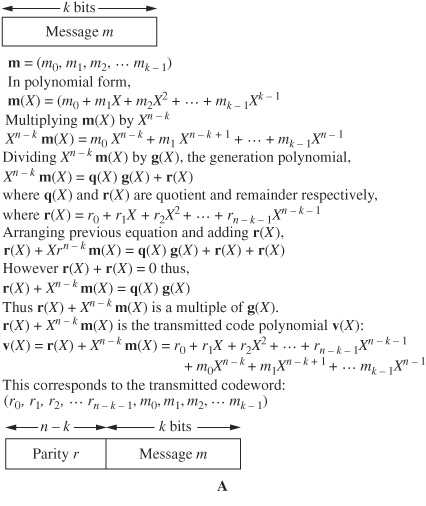
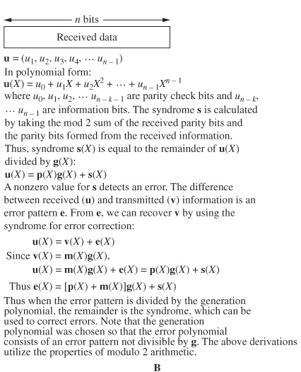
FIGURE 5.6 CRCC encoding and decoding algorithms. A. CRCC encoding. B. CRCC decoding and syndrome calculation.

Error correction can be accomplished by forming an error pattern that is the difference between the received data and the original data to be recovered. This is mathematically possible because the error polynomial e divided by the original generation polynomial produces the syndrome as a remainder. Thus, the syndrome can be used to form the error pattern and hence recover the original data. It is important to select the generation polynomial g so that error patterns in the error polynomial e are not exactly divisible by g. CRCC will fail to detect an error if the error is exactly divisible by the generation polynomial.

In practice, CRCC and other detection and correction codewords are described in mathematical terms, where the data bits are treated as the coefficients of a binary polynomial. As we observed in Chap. 1, the binary number system is one of positional notation such that each place represents a power of 2. Thus, we can write binary numbers in a power of 2 notation. For example, the number 1001011, with MSB (most significant bit) leading, can be expressed as:

1× 2⁶ + 0× 2⁵ + 0× 2⁴ + 1× 2³ + 0× 2² + 1× 2¹ + 1× 2⁰

or:

2⁶ + 2³ + 2¹ + 2⁰

In general, the number can be expressed as:

x⁶ + x³ + x + 1

With LSB (least significant bit) leading, the notation would be reversed. This polynomial notation is the standard terminology in the field of error correction. In the same way that use of modulo arithmetic ensures that all possible numbers will fall in the modulus, polynomials are used to ensure that all values fall within a given range. In modulo arithmetic, all numbers are divided by the modulus and the remainder is used as the number. Similarly, all polynomials are divided by a modulus polynomial of degree n. The remainder has n coefficients, and is recognizable as a code symbol. Further, just as we desire a modulus that is a prime number (so that when a product is 0, at least one factor is 0), we desire a prime polynomial—one that cannot be represented as the product of two polynomials. The benefit is added structure to devised codes, resulting in more efficient implementation.

Using polynomial notation, we can see how CRCC works. An example of cyclic code encoding is shown in Fig. 5.7. The message 1001 is written as the polynomial x³ + 1. So that three parity check bits can be appended, the message is multiplied by x³ to shift the data to the left. The message is then divided by the generation polynomial x³ + x² + 1. The remainder x + 1 is appended to create the polynomial x⁶ + x³ + x + 1.

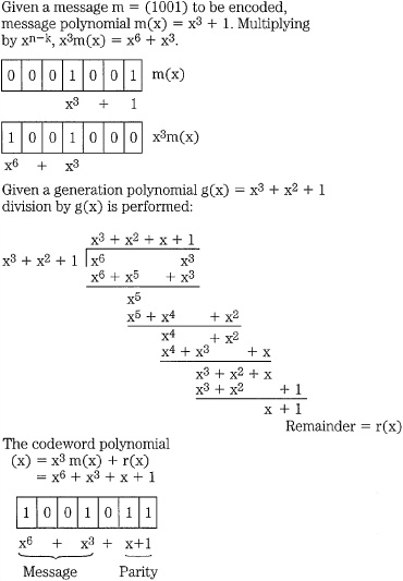
FIGURE 5.7 An example of cyclic code encoding, with message 1001 written as the polynomial x³ + 1. The encoder outputs the original message and a parity word.

x + 1.

A shift register implementation of this encoder is shown in Fig. 5.8. The register is initially loaded with 0s, and the four message bits are sequentially shifted into the register, and appear at the output. When the last message bit has been output, the encoder’s switches are switched, 0s enter the register, and three parity bits are output. Modulo 2 adders are used. This example points up an advantage of this type of error-detection encoding: the implementation can be quite simple.

The larger the data block, the less redundancy results, yet mathematical analysis shows that the same error-detection capability remains. However, if random or short duration burst errors tend to occur frequently, then the integrity of the detection is decreased and shorter blocks might be necessitated. The extent of error detectability of a CRCC code can be summarized. Given a k-bit data word with m (where m = n − k) bits of CRCC, a codeword of n bits is formed, and the following are true:

• Burst errors less than or equal to m bits are always detectable.

• Detection probability of burst errors of m + 1 bits is 1 − 2^{−m + 1}.

• Detection probability of burst errors longer than m + 1 bits is 1 − 2^−m. (These first three items are not affected by the length n of the codeword.)

• Random errors up to three consecutive bits long can be detected.

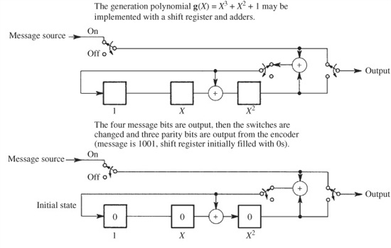
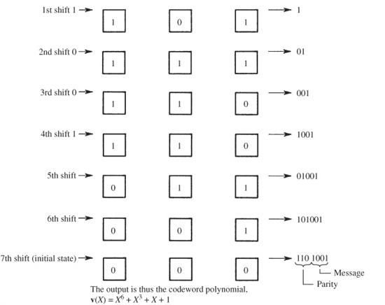
FIGURE 5.8 An implementation of a cyclic encoder using shift registers. Modulo 2 (XOR) adders are used.

CRCC is quite reliable. For example, if 16 parity check bits are generated, the probability of error detection is 1 − 2⁻¹⁶ or about 99.99%. Ultimately, the medium determines the design of the CRCC and the rest of the error-correction system. The power of the error-correction processing following the CRCC also influences how accurate the CRCC detection must be. The CRCC is often used as an error pointer to identify the number and extent of errors prior to other error-correction processing. In some cases, to reduce codeword size, a shortened or punctured code is used. In this technique, some of the leading bits of the codeword are omitted.

The techniques used in the CRCC algorithm apply generally to cyclic error-detection and error-correction algorithms. They use codewords that are polynomials that normally result in a zero remainder when divided by a generation polynomial. To perform error checking on received data, division is performed; a zero remainder syndrome indicates that there is no error. A nonzero remainder syndrome indicates an error. The nonzero syndrome is the error polynomial divided by the check polynomial. The syndrome can be used to correct the error by multiplying the syndrome by the check polynomial to obtain the error polynomial. The error in the received data appears as the error polynomial added to the original codeword. The correct original codeword can be obtained by subtracting (adding in modulo 2) the error polynomial from the received polynomial.

Error-Correction Codes

With the help of redundant data, it is possible to correct errors that occur during the storage or transmission of digital audio data. In the simplest case, data is merely duplicated. For example, instead of writing only one data track, two tracks of identical data could be written. The first track would normally be used for playback, but if an error was detected through parity or other means, data could be taken from the second track. To alleviate the problem of simultaneously erroneous data, redundant samples could be displaced with respect to each other in time.

In addition, channel coding can be used beneficially. For example, 3-bit words can be coded as 7-bit words, selected from 2⁷ possible combinations to be as mutually different as possible. The receiver examines the 7-bit words and compares them to the eight allowed codewords. Errors could be detected, and the words changed to the nearest allowed codeword, before the codeword is decoded to the original 3-bit sequence. Four correction bits are required for every three data bits; the method can correct a single error in a 7-bit block. This minimum length concept is important in more sophisticated error-correction codes.

Although such simple methods are workable, they are inefficient because of the data overhead that they require. A more enlightened approach is that of error-correction codes, which can achieve more reliable results with less redundancy. In the same way that redundant data in the form of parity check bits is used for error detection, redundant data is used to form codes for error correction. Digital audio data is encoded with related detection and correction algorithms. On playback, errors are identified and corrected by the detection and correction decoder. Coded redundant data is the essence of all correction codes; however, there are many types of codes, different in their designs and functions.

The field of error-correction codes is a highly mathematical one. Many types of codes have been developed for different applications. In general, two approaches are used: block codes using algebraic methods, and convolutional codes using probabilistic methods. Block codes form a coded message based solely on the message parsed into a data block. In a convolutional code, the coded message is formed from the message present in the encoder at that time as well as previous message data. In some cases, algorithms use a block code in a convolutional structure known as a Cross-Interleave Code. For example, such codes are used in the CD format.

Block Codes

Block error-correction encoders assemble a number of data words to form a block and, operating over that block, generate one or more parity words and append them to the block. During decoding, an algorithm forms a syndrome word that detects errors and, given sufficient redundancy, corrects them. Such algorithms are effective against errors encountered in digital audio applications. Error correction is enhanced by interleaving consecutive words. Block codes base their parity calculations on an entire block of information to form parity words. In addition, parity can be formed from individual words in the block, using single-bit parity or a cyclic code. In this way, greater redundancy is achieved and correction is improved. For example, CRCC could be used to detect an error, then block parity used to correct the error.

A block code can be conceived as a binary message consolidated into a block, with row and column parity. Any single-word error will cause one row and one column to be in error; thus, the erroneous data can be corrected. For example, a message might be grouped into four 8-bit words (called symbols). A parity bit is added to each row and a parity word added to each column, as shown in Fig. 5.9. At the decoder, the data is checked for correct parity, and any single-symbol error is corrected. In this example, bit parity shows that word three is in error, and word parity is used to correct the symbol. A double-word error can be detected, but not corrected. Larger numbers of errors might result in misdetection or miscorrection.

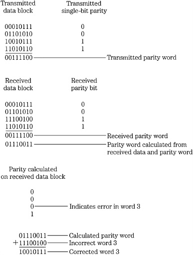
FIGURE 5.9 An example of block parity with row parity bits and a column parity word.

Block correction codes use many methods to generate the transmitted codeword and its parity; however, they are fundamentally identical in that only information from the block itself is used to generate the code. The extent of the correction capabilities of block correction codes can be simply illustrated with decimal examples. Given a block of six data words, a 7th parity word can be calculated by adding the six data words. To check for an error, a syndrome is created by comparing (subtracting in the example) the parity (sum) of the received data with the received parity value. If the result is zero, then most probably no error has occurred, as shown in Fig. 5.10A. If one data word is detected and the word is set to zero, a condition called a single erasure, a nonzero syndrome indicates that; furthermore, the erasure value can be obtained from the syndrome. If CRCC or single-bit parity is used, it points out the erroneous word, and the correct value can be calculated using the syndrome, as shown in Fig. 5.10B. Even if detection itself is in error and falsely creates an error pointer, the syndrome yields the correct result, as shown in Fig. 5.10C. Such a block correction code is capable of detecting a one-word error, or making one erasure correction, or correcting one error with a pointer. The correction ability depends on the detection ability of pointers. In this case, unless the error is identified with a pointer, erasure, or CRCC detection, the error cannot be corrected.

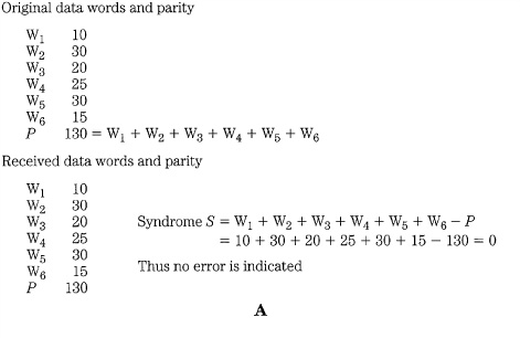
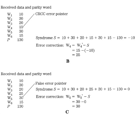
FIGURE 5.10 Examples of single-parity block coding. A. Block correction code showing no error condition. B. Block correction code showing a correction with a pointer. C. Block correction code showing a false pointer.

For enhanced performance, two parity words can be formed to protect the data block. For example, one parity word might be the sum of the data and the second parity word the weighted sum as shown in Fig. 5.11A. If any two words are erroneous and marked with pointers, the code provides correction. Similarly, if any two words are marked with erasure, the code can use the two syndromes to correct the data. Unlike the single parity example, this double parity code can also correct any one-word error, even if it is not identified with a pointer, as shown in Fig. 5.11B. This type of error correction is well-suited for audio applications.

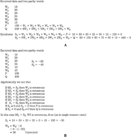
FIGURE 5.11 Examples of double-parity block coding. A. Block correction code with double parity showing no error condition. B. Block correction code with double parity showing a single-error correction without a pointer.

Hamming Codes

Cyclic codes such as CRCC are a subclass of linear block codes, which can be used for error correction. Special block codes, known as Hamming codes, create syndromes that point to the location of the error. Multiple parity bits are formed for each data word, with unique encoding. For example, three parity check bits (4, 5, and 6) might be added to a 4-bit data word (0, 1, 2, and 3); seven bits are then transmitted. For example, suppose that the three parity bits are uniquely defined as follows: parity bit 4 is formed from modulo 2 addition of data bits 1, 2, and 3; parity bit 5 is formed from data bits 0, 2, and 3; and parity bit 6 is formed from data bits 0, 1, and 3. Thus, the data word 1100, appended with parity bits 110, is transmitted as the 7-bit codeword 1100110. A table of data and parity bits is shown in Fig. 5.12A.

This algorithm for calculating parity bits is summarized in Fig. 5.12B. An error in a received data word can be located by examining which of the parity bits detects an error. The received data must be correctly decoded; therefore, parity check decoding equations must be written. These equations are computationally represented as a parity check matrix H, as shown in Fig. 5.12C. Each row of H represents one of the original encoding equations. By testing the received data against the values in H, the location of the error can be identified. Specifically, a syndrome is calculated from the modulo 2 addition of the parity calculated from the received data and the received parity. An error generates a 1; otherwise a 0 is generated. The resulting error pattern is matched in the H matrix to locate the erroneous bit. For example, if the codeword 1100110 is transmitted, but 1000110 is received, the syndromes will detect the error and generate a 101 error pattern. Matching this against the H matrix, we see that it corresponds to the second column; thus, bit 1 is in error, as shown in Fig. 5.12D. This algorithm is a single-error correcting code; therefore, it can correctly identify and correct any single-bit error.

Returning to the design of this particular code, we can observe another of its interesting properties. Referring again to Fig. 5.12A, recall that the 7-bit data words each comprise four data bits and three parity bits. These seven bits provide 128 different encoding possibilities, but only 16 of them are used; thus, 112 patterns are clearly illegal, and their presence would denote an error. In this way, the patterns of bits themselves are useful. We also may ask the question: How many bits must change value for one word in the table to become another word in the table? For example, we can see that three bits in the word 0101010 must change for it to become 0110011. Similarly, we observe that any word in the table would require at least three bit changes to become any other word. This is important because this dissimilarity in data corresponds to the code’s error-correction ability. The more words that are disallowed, the more robust the detection and correction. For example, if we receive a word 1110101, which differs from a legal word 1010101 by one bit, the correct word can be determined. In other words, any single-bit error leaves the received word closer to the correct word than any other.

The number of bits that one legal word must change to become another legal word is known as the Hamming distance, or minimum distance. In this example, the Hamming distance is 3. Hamming distance thus defines the potential error correctability of a code. A distance of 1 determines simple uniqueness of a code. A distance of 2 provides single-error detectability. A distance of 3 provides single-error correctability or double-error detection. A distance of 4 provides both single-error correction and double-error detection, or triple-error detection alone. A distance of 5 provides double-error correction. As the distance increases, so does the correctability of the code.

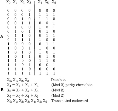
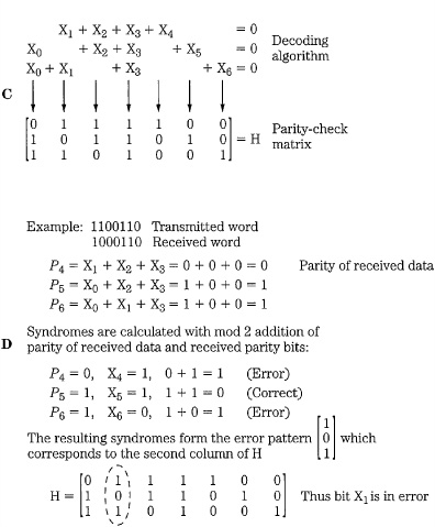
FIGURE 5.12 With Hamming codes, the syndrome points to the error location. A. In this example with four data bits and three parity bits, the code has a Hamming distance of 3. B. Parity bits are formed in the encoder. C. Parity-check matrix in the decoder. D. Single-error correction using a syndrome to point to the error location.

The greater the correctability required, the greater the distance the code must possess. In general, to detect t_d number of errors, the minimum distance required is greater than or equal to t_d + 1. In the case of an erasure e (when an error location is known and set to zero), the minimum distance is greater than or equal to e + 1. To correct all combinations of t_c or fewer errors, the minimum distance required is greater than or equal to 2t_c + 1. For a combination of error correction, the minimum distance is greater than or equal to t_d + e + 2t_c + 1. These hold true for both bit-oriented and word-oriented codes. If m parity blocks are included in a block code, the minimum distance is less than or equal to m + 1. For the maximum-distance separable (MDS) codes such as B-adja-cent and Reed–Solomon codes, the minimum distance is equal to m + 1.

Block codes are notated in terms of the input relative to the output data. Data is grouped in symbols; the smallest symbol is one-bit long. A message of k symbols is used to generate a larger n-bit symbol. Such a code is notated as (n, k). For example, if 12 symbols are input to an encoder and 20 symbols are output, the code would be (20,12). In other words n − k, or eight parity symbols are generated. The source rate R is defined as k/n; in this example, R = 12/20.

Convolutional Codes

Convolutional codes, sometimes called recurrent codes, differ from block codes in the way data is grouped for coding. Instead of dividing the message data into blocks of k digits and generating a block of n code digits, convolutional codes do not partition data into blocks. Instead, message digits k are taken a few at a time and used to generate coded digits n, formed not only from those k message digits, but from many previous k digits as well, saved in delay memories. In this way, the coded output contains a history of the previous input data. Such a code is called an (n, k) convolutional code. It uses (N − 1) message blocks with k digits. It has constraint length N blocks (or nN digits) equal to n(m + 1), where m is the number of delays. Its rate R is k/n.

As with linear block codes, encoding is performed and codewords are transmitted or stored. Upon retrieval, the correction decoder uses syndromes to check codewords for errors. Shift registers can be used to implement the delay memories required in the encoder and decoder. The amount of delay determines the code’s constraint length, which is analogous to the block length of a block code. An example of a convolutional encoder is shown in Fig. 5.13. There are six delays, thus the constraint length is 14. The other parameters are q = 2, R = 1/2, k = 1, n = 2, and the polynomial is x⁶ + x⁵ + x² + 1. As shown in the diagram, message data passes through the encoder, so that previous bits affect the current coded output.

Another example of a convolutional encoder is shown in Fig. 5.14A. The upper code is formed from input data with the polynomial x² + x + 1, and the lower with x² + 1. The data sequence enters the circuit from the left and is shifted to the right one bit at a time. The two sequences generated from the original sequence with modulo 2 addition are multiplexed to again form a single coded data stream. The resultant code has a memory of two because, in addition to the current input bit, it also acts on the preceding two bits. For every input bit, there are two output bits; hence the code’s rate is 1/2. The constraint length of this code is k = 3.

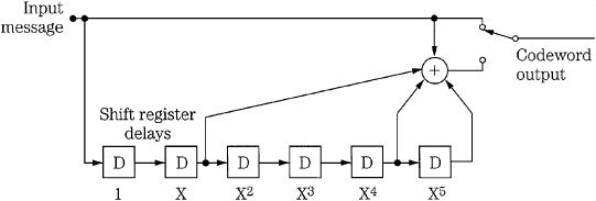
FIGURE 5.13 A convolutional code encoder with six delay blocks.

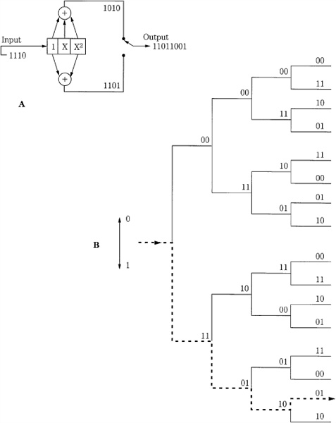
FIGURE 5.14 An example of convolutional encoding. A. Convolutional encoder with k = 3 and R = 1/2. B. Convolutional code tree diagram. (Viterbi, 1983)

A convolutional code can be analyzed with a tree diagram as shown in Fig. 5.14B. It represents the first four sequences of an infinite tree, with nodes spaced n digits apart and with 2k branches leaving each node. Each branch is an n-digit code block that corresponds to a specific k-digit message block. Any codeword sequence is represented as a path through the tree. For example, the encoded sequence for the previous encoder example can be traced through the tree. If the input bit is a 0, the code symbol is obtained by going up to the next tree branch; if the input is a 1, the code symbol is obtained by going down. The input message thus dictates the path through the tree, each input digit giving one instruction. The sequence of selections at the nodes forms the output codeword. From the previous example, the input 1110 generates the output path 11011001. Upon playback, the data is sequentially decoded and errors can be detected and recovered by comparing all possible transmitted sequences to those actually received. The received sequence is compared to transmitted sequences, branch by branch. The decoding path through the tree is guided by the algorithm, to find the transmitted sequence that most likely gave rise to the received sequence.

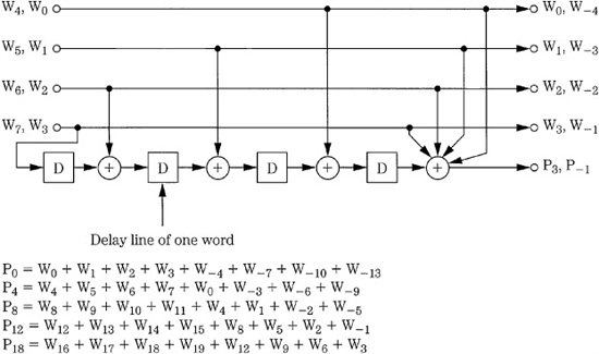
FIGURE 5.15 An example of a convolutional code encoder, generating one check word for every four data words. (Doi, 1983)

Another convolutional code is shown in Fig. 5.15. Here, the encoder uses four delays, each with a duration of one word. Parity words are generated after every four data words, and each parity word has encoded information derived from the previous eight data words. The constraint length of the code is 14. Convolutional codes are often inexpensive to implement, and perform well under high error conditions. One disadvantage of convolutional codes is error propagation; an error that cannot be fully corrected generates syndromes reflecting this error, and this can introduce errors in subsequent decoding. Convolutional codes are not typically used with recorded data, particularly when editing is required; the discrete nature of block codes makes them more suitable for this. Convolutional codes are more often used in broadcast and wireless applications.

Interleaving

Error correction depends on an algorithm’s ability to overcome erroneous data. When the error is sustained, as in the case of a burst error, large amounts of continuous data as well as redundant data may be lost, and correction may be difficult or impossible. To overcome this, data is often interleaved or dispersed through the data stream prior to storage or transmission. If a burst error occurs after the interleaving stage, it damages a continuous section of data. However, on playback, the bitstream is de-interleaved; thus, the data is returned to its original sequence and conversely the errors are distributed through the bitstream. With valid data and valid redundancy now surrounding the damaged data, the algorithm is better able to reconstruct the damaged data. Figure 5.16 shows an example of interleaving and de-interleaving, with a burst error occurring during storage or transmission. Following de-interleaving, the errors have been dispersed, facilitating error correction.

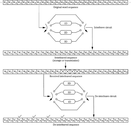
FIGURE 5.16 Zero-, one-, two-, and three-word delays perform interleaving and de-interleaving for error dispersion prior to correction. (Doi, 1983)

Interleaving provides an important advantage. Without interleaving, the amount of redundancy would be dictated by the size of the largest correctable burst error. With interleaving, the largest error that can occur in any block is limited to the size of the interleaved sections. Thus, the amount of redundancy is determined not by burst size, but by the size of the interleaved section. Simple delay interleaving effectively disperses data. Many block checksums work properly if there is only one word error per block. A burst error exceeds this limitation; however, interleaved and de-interleaved data may yield only one erroneous word in a given block. Thus, interleaving greatly increases burst-error correctability of block codes. Bit interleaving accomplishes much the same purpose as block interleaving: it permits burst errors to be handled as shorter burst errors or random errors. Any interleaving process requires a buffer long enough to hold the distributed data during both interleaving and de-interleaving.

Cross-Interleaving

Interleaving may not be adequate when burst errors are accompanied by random errors. Although the burst is scattered, the random errors add additional errors in a given word, perhaps overloading the correction algorithm. One solution is to generate two correction codes, separated by an interleave and delay. When block codes are arranged in rows and columns two-dimensionally, the code is called a product code (or cross word code). The minimum distance is the product of the distances of each code. When two block codes are separated by both interleaving and delay, cross-interleaving results. In other words, a Cross-Interleave Code (CIC) comprises two (or more) block codes assembled with a convolutional structure, as shown in Fig. 5.17. The method is efficient because the syndromes from one code can be used to point to errors, which are corrected by the other code. Because error location is known, correctability is enhanced. For example, a random error is corrected by the interleaved code, and a burst error is corrected after de-interleaving. When both codes are single-erasure correcting codes, the resulting code is known as a Cross-Interleave Code. In the Compact Disc format, Reed–Solomon codes are used and the algorithm is known as the Cross-Interleave Reed–Solomon code (CIRC). Product codes are used in the DVD and Blu-ray formats.

An example of a simple CIC encoder is shown in Fig. 5.18. The delay units produce interleaving, and the modulo 2 adders generate single-erasure correcting codes. Two parity words (P and Q) are generated, and with two single-erasure codes, errors are efficiently corrected. Triple-word errors can be corrected; however, four-word errors produce double-word errors in all four of the generated sequences, and correction is impossible. The CIC enjoys the high performance of a convolutional code but without error propagation, because any uncorrectable error in one sequence always becomes a one-word error in the next sequence and thus can be easily corrected.

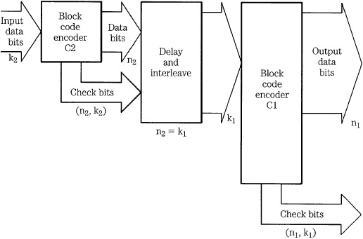
FIGURE 5.17 A cross-interleave code encoder. Syndromes from the first block are used as error pointers in the second block. In the CD format, k₂ = 24, n₂ = 28, k₁ = 28, and n₁ = 32; the C1 and C2 codes are Reed–Solomon codes.

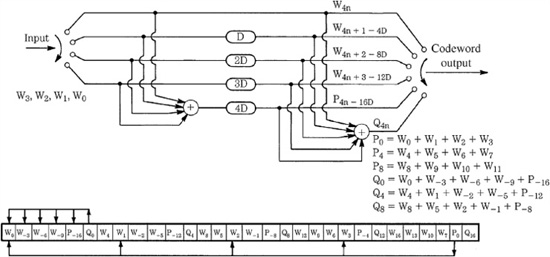
FIGURE 5.18 An example of a CIC encoder and its output sequence. (Doi, 1983)

Reed–Solomon Codes

Reed–Solomon codes were devised by Irving Reed and Gustave Solomon in 1960, at the Massachusetts Institute of Technology, Lincoln Laboratories. They are an example of an important subclass of codes known as q-ary BCH codes, devised by Raj Chandra Bose, Dwijendra Kumar Ray-Chaudhuri, and Alexis Hocquenghem in 1959 and 1960. BCH codes are a subclass of Hamming codes. Reed–Solomon codes are cyclic codes that provide multiple-error correction. They provide maximum correcting efficiency. They define code symbols from n-bit bytes, with codewords consisting of 2ⁿ − 1 of the n-bit bytes. If the error pattern affects s bytes in a codeword, 2s bytes are required for error correction. Thus 2ⁿ − 1 − 2s bytes are available for data. When combined with cross-interleaving, Reed–Solomon codes are effective for audio applications because the architecture can correct both random and burst errors.

Reed–Solomon codes exclusively use polynomials derived using finite field mathematics known as Galois Fields (GF) to encode and decode block data. Galois Fields, named in honor of the extraordinary mathematical genius Evariste Galois (who devised them before his death in a duel at age 20), comprise a finite number of elements with special properties. Either multiplication or addition can be used to combine elements, and the result of adding or multiplying two elements is always a third element contained in the field. For example, when an element is raised to higher powers, the result is always another element in the field. Such fields generally only exist when the number of elements is a prime number or a power of a prime number. In addition, there exists at least one element called a primitive such that every other element can be expressed as a power of this element.

For error correction, Galois Fields yield a highly structured code, which ultimately simplifies implementation of the code. In Reed–Solomon codes, data is formed into symbols that are members of the Galois Field used by the code; Reed–Solomon codes are thus nonbinary BCH codes. They achieve the greatest possible minimum distance for the specified input and output block lengths. The minimum distance, the number of nonbinary symbols in which the sequences differ, is given by: d = n − k + 1. The size of the Galois Field, which determines the number of symbols in the code, is based on the number of bits comprising a symbol; 8-bit symbols are commonly used. The code thus contains 2⁸ − 1 or 255 8-bit symbols. A primitive polynomial often used in GF(2⁸) systems is x⁸ + x⁴ + x³ + x² + 1.

Reed–Solomon codes use multiple polynomials with roots that locate multiple errors and provide syndromes to correct errors. For example, the code can use the input word to generate two parity polynomials, P and Q. The P parity can be a modulo 2 sum of the symbols. The Q parity multiplies each input word by a different power of the GF primitive element. If one symbol is erroneous, the P parity gives a nonzero syndrome S₁. The Q parity yields a syndrome S₂; its value is S₁, raised to a power—the value depending on the position of the error. By checking this relationship between S₁ and S₂, the Reed–Solomon code can locate the error. When a placed symbol is in error, S₂ would equal S₁ multiplied by the element raised to the placed power. Correction is performed by adding S₁ to the designated location. This correction is shown in the example below. Alternatively, if the position of two errors is already known through detection pointers, then two errors in the input can be corrected. For example, if the second and third symbols are flagged, then S₁ is the modulo 2 sum of both errors, and S₂ is the sum of the errors multiplied by the second and third powers.

To illustrate the operation of a Reed–Solomon code, consider a GF(2³) code comprising 3-bit symbols. In this code, a is the primitive element and is the solution to the equation:

F(x) = x³ + x + 1 = 0

such that an irreducible polynomial can be written:

α³ + α + 1 = 0

where + indicates modulo 2 addition. The elements can be represented as ordinary polynomials:

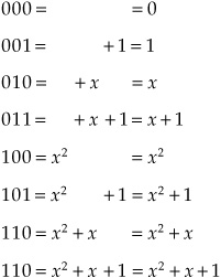
Because = x, using the properties of the Galois Field and modulo 2 (where 1 + 1 = + = ² + ² = 0) we can create a logarithmic representation of the irreducible polynomial elements in the field where the bit positions indicate polynomial positions:

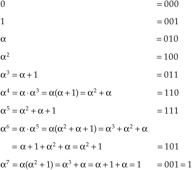
In this way, all possible 3-bit symbols can be expressed as elements of the field (0, 1 = ⁷, , ², ³, ⁴, ⁵, and ⁶) where is the primitive element (010). Elements can be multiplied by simply adding exponents, always resulting in another element in the Galois Field. For example:

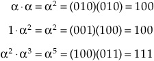
The complete product table for this example GF(2³) code is shown in Fig. 5.19; the modulo ⁷ results can be seen. For example, ^{4 6} = ¹⁰, or ³. Using the irreducible polynomials and the product table, the correction code can be constructed. Suppose that A, B, C, and D are data symbols and P and Q are parity symbols. The Reed–Solomon code will satisfy the following equations:

Using the devised product laws, we can solve these equations to yield:

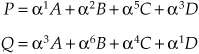
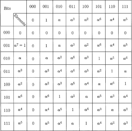
FIGURE 5.19 The product table for a GF(2³) code with F(x) = x³ + x + 1 and primitive element 010.

For example, given the irreducible polynomial table, if:

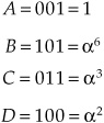
we can solve for P and Q using the product table:

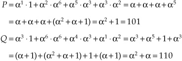
Thus:

P = 101 = α⁶

Q = 110 = α⁴

Errors in received data can be corrected using syndromes, where a prime () indicates received data:

If each possible error pattern is expressed by E_i, we write the following:

If there is no error, then S₁ = S₂ = 0.

If symbol A is erroneous, S₁ = E_A and S₂ = ⁶S₁.

If symbol B is erroneous, S₁ = E_B and S₂ = ⁵S₁.

If symbol C is erroneous, S₁ = E_C and S₂ = ⁴S₁.

If symbol D is erroneous, S₁ = E_D and S₂ = ³S₁.

If symbol P is erroneous, S₁ = E_P and S₂ = ²S₁.

If symbol Q is erroneous, S₁ = E_Q and S₂ = ¹S₁.

In other words, an error results in nonzero syndromes; the value of the erroneous symbols can be determined by the difference of the weighting between S₁ and S₂. The ratio of weighting for each word is different thus single-word error correction is possible. Double erasures can be corrected because there are two equations with two unknowns. For example, if this data is received:

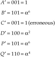
We can calculate the syndromes (recalling that 1 + 1 = + = ² + ² = 0):

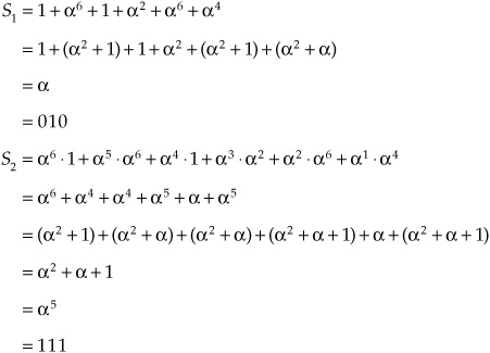
Because S₂ = ⁴S₁ (that is, ⁵ = ⁴ ·), symbol C must be erroneous and because S₁ = E_C = 010, C = C + E_C = 001 + 010 = 011, thus correcting the error.

In practice, the polynomials used in CIRC are:

P + α⁶A + α¹B + α²C + α⁵D + α³E

Q + α²A + α³B + α⁶C + α⁴D + α¹E

and the syndromes are:

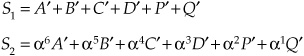
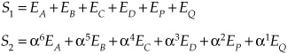
S₁ = A′ + B′ + C′ + D′ + E′ + P′ + Q′

S₂ = α⁷A′ + α⁶B′ + α⁵C′ + α⁴D′ + α³E′ + α²P′ + α¹Q′

Because Reed–Solomon codes are particularly effective in correcting burst errors, they are highly successful in digital audio applications when coupled with error-detection pointers such as CRCC and interleaving. Reed–Solomon codes are used for error correction in applications such as CD, DVD, Blu-ray, direct broadcast satellite, digital radio, and digital television.

Cross-Interleave Reed–Solomon Code (CIRC)

The Cross-Interleave Reed–Solomon Code (CIRC) is a quadruple-erasure (double-error) correction code that is used in the Compact Disc format. CIRC applies Reed–Solomon codes sequentially with an interleaving process between C2 and C1 encoding. Encoding carries data through the C2 encoder, then the C1 encoder. Decoding reverses the process.

In CIRC, C2 is a (28,24) code, that is, the encoder inputs 24 symbols, 28 symbols (including four parity symbols) are output. C1 is a (32,28) code; the encoder inputs 28 symbols, and 32 symbols (with four additional parity symbols) are output. In both cases, because 8-bit bytes are used, the size of the Galois Field is GF(2⁸); the calculation is based on the primitive polynomial: x⁸ + x⁴ + x³ + x² + 1. Minimum distance is 5. Up to four symbols can be corrected if the error location is known, and two symbols can be corrected if the location is not known.

Using a combination of interleaving and parity to make the data more robust against errors encountered during storage on a CD, the data is encoded before being placed on the disc, and then decoded upon playback. The CIRC encoding algorithm is shown in Fig. 5.20; the similarity to the general structure shown in Fig. 5.17 is evident. Using this encoding algorithm, symbols from the audio signal are cross-interleaved, and Reed–Solomon encoding stages generate P and Q parity symbols.

The CIRC encoder accepts twenty-four 8-bit symbols, that is, 12 symbols (six 16-bit samples) from the left channel and 12 from the right channel. Interestingly, the value of 12 was selected by the designers because it has common multiples of 2, 3, and 4; this would have allowed the CD to more easily also offer 3- or 4-channel implementations—a potential that never came to fruition. An interleaving stage assists interpolation. A two-symbol delay is placed between even and odd samples. Because even samples are delayed by two blocks, interpolation is possible where two uncorrectable blocks occur. The symbols are scrambled to separate even- and odd-numbered symbols; this process assists concealment. The 24-byte parallel word is input to the C2 encoder that produces four symbols of Q parity. Q parity is designed to correct one erroneous symbol, or up to four erasures in one word. By placing the parity symbols in the center of the block, the odd/even distance is increased. This permits interpolation over the largest possible burst error.

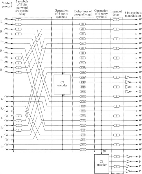
FIGURE 5.20 The CIRC encoding algorithm.

In the cross-interleaving stage, 28 symbols are delayed by differing periods. These periods are integer multiples of four blocks. This convolutional interleave stores one C2 word in 28 different blocks, stored over a distance of 109 blocks. In this way, the data array is crossed in two directions. Because the delays are long and of unequal duration, correction of burst errors is facilitated. Twenty-eight symbols (from 28 different C2 words) are input to the C1 encoder, producing four P parity symbols. P parity is designed to correct single-symbol errors and detect and flag double and triple errors for Q correction.

An interleave stage delays alternate symbols by one symbol. This odd/even delay spreads the output symbols over two data blocks. In this way, random errors cannot corrupt more than one symbol in one word even if there are two erroneous adjacent symbols in one block. The P and Q parity symbols are inverted to provide nonzero P and Q symbols with zero data. Thirty-two 8-bit symbols leave the CIRC encoder.

The error processing must be decoded each time the disc is played to de-interleave the data, and perform error detection and correction. When a Reed–Solomon decoder receives a data block (consisting of the original data symbols plus the parity symbols) it uses the received data to recalculate the parity symbols. If the recalculated parity symbols match the received parity symbols, the block is assumed to be error-free. If they differ, the difference syndromes are used to locate the error. Erroneous words are flagged, for example, as being correctable, uncorrectable, or possibly correctable. Analysis of the flags determines whether the errors are to be corrected by the correction code, or passed on for interpolation. The CIRC decoding algorithm is shown in Fig. 5.21.

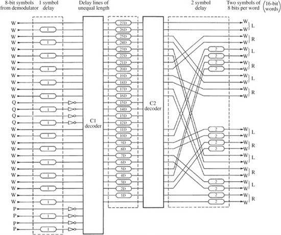
FIGURE 5.21 The CIRC decoding algorithm.

A frame of thirty-two 8-bit symbols is input to the CIRC decoder: twenty-four are audio symbols and eight are parity symbols. Odd-numbered symbols are passed through a one-symbol delay. In this way, even-numbered symbols in a frame are de-interleaved with the odd-numbered symbols in the next frame. Audio symbols are restored to their original order and disc errors are scattered. This benefits C1 correction, especially for small errors in adjoining symbols. Following this de-interleaving, parity symbols are inverted.

Using four P parity symbols, the C1 decoder corrects random errors and detects burst errors. The C1 decoder can correct one erroneous symbol in each frame. If there is more than one erroneous symbol, the 28 data symbols are marked with an erasure flag and passed to the C2 decoder. Valid symbols are passed along unprocessed. Convolutional de-interleaving between the decoders enables the C2 decoder to correct long burst errors. The frame input to C2 contains symbols from C1 decoded at different times; thus, symbols marked with an erasure flag are scattered. This assists the C2 decoder in correcting burst errors. Symbols without a flag are assumed to be error-free, and are passed through unprocessed.

Given precorrected data, and help from de-interleaving, C2 can correct burst errors as well as random errors that C1 was unable to correct. Using four Q parity symbols, C2 can detect and correct single-symbol errors and correct up to four symbols, as well as any symbols miscorrected by C1 decoding. C2 also can correct errors that might occur in the encoding process itself, rather than on the disc. When C2 cannot accomplish correction, for example, when more than four symbols are flagged, the 24 data symbols are flagged and passed on for interpolation. Final descrambling and delay completes CIRC decoding.

CIRC Performance Criteria

The integrity of data stored on a CD and passing through a CIRC algorithm can be assessed through a number of error counts. Using a two-digit nomenclature, the first digit specifies the number of erroneous symbols (bytes), and the second digit specifies at which decoder (C1 or C2) they occurred. Three error counts (E11, E21, and E31) are measured at the output of the C1 decoder. The E11 count specifies the frequency of occurrence of single-symbol (correctable) errors per second in the C1 decoder. E21 indicates the frequency of occurrence of double-symbol (correctable) errors in the C1 decoder. E31 indicates the frequency of triple-symbol (uncorrectable at C1) errors in the C1 decoder. E11 and E21 errors are corrected in the C1 stage. E31 errors are uncorrected in the C1 stage, and are passed along to the second C2 stage of correction.

There are three error counts (E12, E22, and E32) at the C2 decoder. The E12 count indicates the frequency of occurrence of a single-symbol (correctable) error in the C2 decoder measured in counts per second. A high E12 count is not problematic because one E31 error can generate up to 30 E12 errors due to interleaving. The E22 count indicates the frequency of two-symbol (correctable) errors in the C2 decoder. E22 errors are the worst correctable errors; the E22 count indicates that the system is close to producing an uncorrectable error; a CD-ROM with 15 E22 errors would be unacceptable even though the errors are correctable. A high E22 count can indicate localized damage to the disc, from manufacturing defect or usage damage. The E32 count indicates three or more symbol (uncorrectable) errors in the C2 decoder, or unreadable data in general; ideally, an E32 count should never occur on a disc. E32 errors are sometimes classified as noise interpolation (NI) errors; when an E32 error occurs, interpolation must be performed. If a disc has no E32 errors, all data is output accurately.

The block-error rate (BLER) measures the number of frames of data that have at least one occurrence of uncorrected symbols (bytes) at the C1 error-correction decoder input (E11 + E21 + E31); it is thus a measure of both correctable and uncorrectable errors at that decoding stage. Errors that are uncorrectable at this stage are passed along to the next error-correction stage. BLER is a good general measure of disc data quality. BLER is specified as rate of errors per second. The CD standard sets a maximum of 220 BLER errors per second averaged over 10 seconds for audio discs; however, a well-manufactured disc will have an average BLER of less than 10. A high BLER count often indicates poor pit geometry that disrupts the pickup’s ability to read data, resulting in many random-bit errors. A high BLER might limit a disc’s lifetime as other scratches accumulate to increase total error count. Likewise a high BLER may cause playback to fail in some players. The CD block rate is 7350 blocks per second; hence, the maximum BLER value of 220 counts per second shows that 3% of frames contain a defect. This defines the acceptable (correctable) error limit; greater frequency might lead to audible faults. The BLER does not provide information on individual defects between 100 and 300 μm, because the BLER responds to defects that are the size of one pit. BLER is often quoted as a 1-second actual value or as a sliding 10-second average across the disc, as well as the maximum BLER encountered during a single 10-second interval during the test.

The E21 and E22 signals can be combined to form a burst-error (BST) count. It counts the number of consecutive C2 block errors exceeding a specified threshold number. It generally indicates a large physical defect on the disc such as a scratch, affecting more than one block of data. For example, if there are 14 consecutive block errors and the threshold is set at seven blocks, two BST errors would be indicated. This count is often tabulated as a total number over an entire disc. A good quality control specification would not allow any burst errors (seven frames) to occur. In practice, a factory-fresh disc might yield BLER = 5, E11 = 5, E21 = 0, and E31 = 0. E32 uncorrectable errors should never occur in a new disc. Figure 5.22 shows an example of the error counts measured from a Compact Disc with good-quality data readout. Error counts are measured vertically, across the duration of this 50-minute disc. As noted above, the high E12 error count is not problematic. Following CIRC error correction, this disc does not have any errors in its output data.

The success of CIRC error correction ultimately depends on the implementation of the algorithm. Generally, CIRC might provide correction of up to 3874 bits, corresponding to a track-length defect of 2.5 mm. Good concealment can extend to 13,282 bits, corresponding to an 8.7-mm defect, and marginal concealment can extend to approximately 15,500 bits.

Product Codes

The CIRC is an example of a cross-interleaved code in which two codes are separated by convolutional interleaving. In two-dimensional product codes, two codes are serially separated by block interleaving. The code that is the first to encode and the last to decode is called the outer C2 code. The code that is the second to encode and the first to decode is called the inner C1 code. Product codes thus use the method of crossing two error-correction codes. If C2 is a (n₂, k₂) block code and C1 is a (n₁, k₁) block code, then they yield a (n₁n₂, k₁k₂) product code with k₁k₂ symbols in an array. The C2 code adds P parity to the block rows, and the C1 code adds Q parity to the block columns as shown in Fig. 5.23. Every column is a codeword of C1. When linear block codes are used, the bottom row words are also codewords of C2. The check data in the lower right-hand corner (intersection of the P column and the Q row) is a check on the check data and can be derived from either column or row check data.

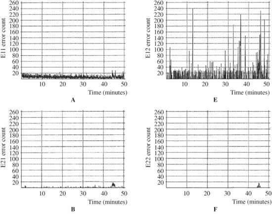
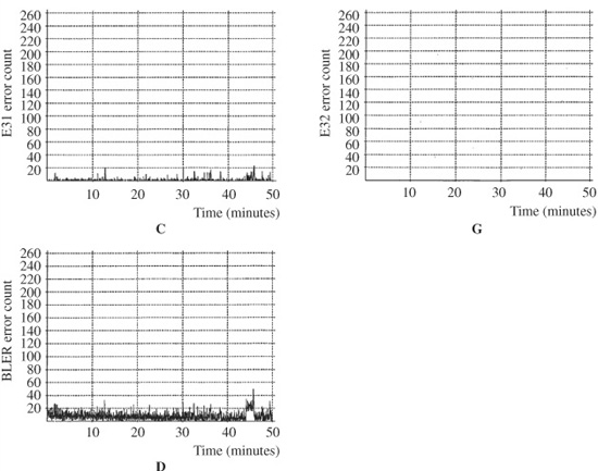
FIGURE 5.22 Example of error counts across a 50-minute Compact Disc. A. E11 error count. B. E21 error count. C. E31 error count. D. BLER error count. E. E12 error count. F. E22 error count. G. E32 error count (no errors).

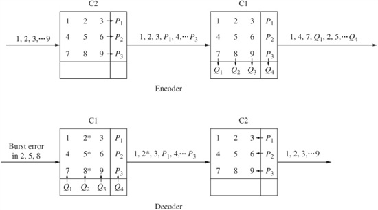
FIGURE 5.23 Block diagram of a product code showing outer-row (P) redundancy and inner-column (Q) redundancy. A burst error is flagged in the C1 decoder and corrected in the C2 decoder.

During decoding, Q parity is used by the C1 decoder to correct random-bit errors, and burst errors are flagged and passed through de-interleaving to the C2 decoder. Symbols are passed through de-interleaving so that burst errors in inner codewords will appear as single-symbol errors in different codewords. The P parity and flags are used by the C2 decoder to correct errors in the inner codewords.

Product codes are used in many audio applications. For example, the DAT format provides an example of a product code in which data is encoded with Reed–Solomon error-correction code over a Galois Field GF(2⁸) using the polynomial x⁸ + x⁴ + x³ + x² + 1. The inner code C1 is a (32,28) Reed–Solomon code with a minimum distance of 5. Four bytes of redundancy are added to the 28 data bytes. The outer code C2 is a (32,26) Reed–Solomon code with a minimum distance of 7. Six bytes of redundancy are added to the 26 data bytes. Both C1 and C2 codes are composed of 32 symbols and are orthogonal with each other. C1 is interleaved over two blocks, and C1 is interleaved across an entire PCM data track, every four blocks. As with the Compact Disc, the error-correction code used in DAT endeavors to detect and correct random errors (using the inner code) and eliminate them prior to de-interleaving; burst errors are detected and flagged. Following de-interleaving, burst errors are scattered and more easily corrected. Using the error flags, the outer code can correct remaining errors. Uncorrected errors must be concealed.

Two blocks of data are assembled in a frame, one from each head, and placed in a memory arranged as 128 columns by 32 bytes. Samples are split into two bytes to form 8-bit symbols. Symbols are placed in memory, reserving a 24-byte wide area in the middle columns. Rows of data are applied to the first (outer C2 code) Reed–Solomon encoder, selecting every fourth column, finishing at column 124 and so yielding 26 bytes. The Reed–Solomon encoder generates six bytes of parity yielding 32 bytes. These are placed in the middle columns, at every fourth location (52, 56, 60, and so on). The encoder repeats its operation with the second column, taking every fourth byte, finishing at column 125. Six parity bytes are generated and placed in every fourth column (53, 57, 61, and so on). Similarly, the memory is filled with 112 outer codewords. (The final eight rows require only two passes because odd-numbered columns have bytes only to row 23.)

Memory is next read by columns. Sixteen even-numbered bytes from the first column, and the first 12 even-numbered bytes from the second column are applied to the second (inner C1 code) encoder, yielding four parity bytes for a total codeword of 32 bytes. This word forms one recorded synchronization block. A second pass reads the odd-numbered row samples from the first two columns of memory, again yielding four parity bytes and another synchronization block. Similarly, the process repeats until 128 blocks have been recorded.

The decoding procedure utilizes first the C1 code, then the C2 code. In C1 decoding, a syndrome is calculated to identify data errors as erroneous symbols. The number of errors in the C1 code is determined using the syndrome; in addition, the position of the errors can be determined. Depending on the number of errors, C1 either corrects the errors or flags the erroneous symbols. In C2 decoding, a syndrome is again calculated, the number and position of errors determined, and the correction is carried out. During C1 decoding, error correction is performed on one or two erroneous bytes due to random errors. For more than two errors, erasure correction is performed using C1 flags attached to all bytes in the block prior to de-interleaving. After de-interleaving, these errors are distributed and appear as single-byte errors with flags. The probability of uncorrectable or misdetected errors increases along with the number of errors in C1 decoding. It is negligible for a single error because all four syndromes will agree on the error. A double error increases the probability.

The C2 decoding procedure is selected to reduce the probability of misdetection. For example, the optimal combination of error correction and erasure correction can be selected on the basis of error conditions. In addition, C2 carries out syndrome computation even when no error flags are received from C1. Because C1 has corrected random errors, C2’s burst-error correction is not compromised. C2 independently corrects one-or two-byte errors in the outer codeword. For two to six erroneous bytes in the outer codeword, C2 uses flags supplied by C1 for erasure correcting. Because the outer code undergoes four-way interleaving, four erroneous synchronization blocks result in only one erroneous byte in an outer codeword. Because C2 can correct up to six erroneous bytes, burst errors up to 24 synchronization blocks in duration can thus be corrected.

Product codes can outperform other codes in modern audio applications; they demand more memory for implementation, but in many applications this is not a serious detriment. Product codes provide good error-correction performance in the presence of simultaneous burst and random errors and are widely used in high-density optical recording media such as DVD and Blu-ray discs. DVD is discussed in Chap. 8 and Blu-ray is discussed in Chap. 9.

Error Concealment

As noted, a theoretically perfect error-detection and error-correction method could be devised in which all errors are completely supplanted with redundant data or calculated with complete accuracy. However, such a scheme would be impractical because of the data overhead. A practical error-correction method balances those limitations against the probability of uncorrected errors and allows severe errors to remain uncorrected. However, subsequent processing—an error-concealment system—compensates for those errors and ensures that they are not audible. Several error-concealment techniques, such as interpolation and muting, have been devised to accomplish this.

Generally, there are two kinds of uncorrectable errors output from correction algorithms. Some errors can be properly detected; however, the algorithm is unable to correct them. Other errors are not detected at all or are miscorrected. The first type of error, detected but not corrected, can usually be concealed with properly designed concealment methods. However, undetected and miscorrected errors often cannot be concealed and may result in an audible click in the audio output. These types of errors, often caused by simultaneous random and burst errors, must be minimized. Thus, an error-correction system aims to reduce undetected errors in the error-correction algorithm, and then relies on the error-concealment methods to resolve detected but not corrected errors.

Interpolation

Following de-interleaving, most errors, even burst errors, are interspersed with valid data words. It is thus reasonable to use techniques in which surrounding valid data is used to calculate new data to replace the missing or uncorrected data. This technique works well, provided that errors are sufficiently dispersed and there is some correlation between data values. Fortunately, digital data comprising a musical selection can often undergo interpolation without adverse audibility. Although it is nonintuitive, studies have shown that within limits, the time duration of an error does not overly affect perception of the error.

In its simplest form, interpolation holds the previous sample value and repeats it to cover the missing or incorrect sample. This is called zero-order or previous-value interpolation. In first-order interpolation, sometimes called linear-order interpolation, the erroneous sample is replaced with a new sample derived from the mean value of the previous and subsequent samples. In many digital audio systems, a combination of zero- and first-order interpolation is used. If consecutive sample errors occur in spite of interleaving, then previous-value interpolation is used to replace consecutive errors, but the final held sample’s value is calculated from the mean value of the held and subsequent sample. If the errors are random, that is, valid samples surround the errors, then mean value calculations are used. One interpolation strategy is shown in Fig. 5.24. Other higher-order interpolation is sometimes used; nth-order interpolation uses a higher-order polynomial to calculate substituted data. In practice, third- and fifth-order interpolations are sometimes used. Clearly, any interpolation calculations must be accomplished quickly enough to maintain the data rate. The results of one experiment in relative values of interpolation noise are shown in Fig. 5.25.

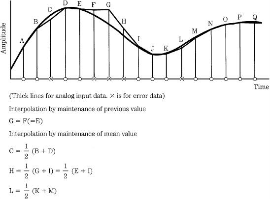
FIGURE 5.24 Interpolation is used to conceal errors. For example, a previous value can be held, followed by a calculation of the mean value.

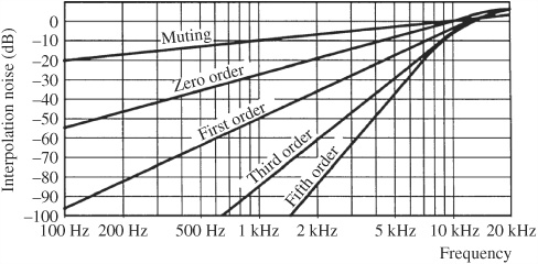
FIGURE 5.25 Noise characteristics for different interpolation methods (for 100-bit burst length, pure tone signals, and uncorrectable errors). (Doi, 1983)

Muting

Muting is the simple process of setting the value of missing or uncorrected words to zero. This silence is preferable to the unpredictable sounds that can result from decoding incorrect data. Muting might be used in the case of uncorrected errors, which would otherwise cause an audible click at the output. The momentary interruption from a brief mute might be imperceptible, but a click would typically be audible. Also, in the case of severe data damage or player malfunction, it is preferable to mute the data output. To minimize audibility of a mute, muting algorithms gradually attenuate the output signal’s amplitude prior to a mute, and then gradually restore the amplitude afterward. For example, gain can be adjusted by multiplying successive samples by attenuation coefficients over a few milliseconds. Of course, gain reduction must begin prior to the error itself, to allow time for a smooth fade. This is easily accomplished by delaying all audio samples briefly and feeding the mute flag forward. Very short-duration muting cannot be perceived by the human ear. Concealment strategies are assisted when audio channels are processed independently, for example, by muting only one channel rather than both.

Duplication

One of the benefits of digital audio recording is the opportunity to copy recordings without the inevitable degradation of analog duplication. Although digital audio duplication can be lossless, its success depends on the success of error correction. Although error-correction methods provide completely correct data, error concealment does not. Under marginal circumstances, error-concealment techniques do introduce audible errors into copied data. Thus, subsequent generations of digital copies could contain an accumulation of concealed errors not present in the original. As a result, errors must be corrected at their origin. Routine precautions of clean media, clean machine mechanisms, and proper low-jitter interfacing are important for digital audio duplication, particularly when many generations of copying are anticipated. In practice, digital audio data can be copied with high reliability. When a file is copied and contains exactly the same values as the original file, it is a clone of the original, with an implicit sampling frequency. Neither the original nor the cloned values have control over the storage media or playback conditions. The copy will sound the same as the original, but only if its playback conditions equal those of the original file’s playback conditions. A simple way to test bit-for-bit accuracy is to load both files into a workstation and exactly synchronize the files to sample accuracy, invert one file and add them. A null result shows bit-for-bit accuracy. Likewise, a residue signal shows the difference between the files.