CHAPTER 11
Low Bit-Rate Coding: Codec Design

In the view of many observers, compared to newer coding methods, linear pulse-code modulation (PCM) is a powerful but inefficient dinosaur. Because of its gargantuan appetite for bits, PCM coding is not suitable for many audio applications. There is an intense desire to achieve lower bit rates because low bit-rate coding opens so many new applications for digital audio (and video). Responding to the need, audio engineers have devised many lossy and lossless codecs. Some codecs use proprietary designs that are kept secret, some are described in standards that can be licensed, while others are open source. In any case, it would be difficult to overstate the importance of low bit-rate codecs. Codecs can be found in countless products used in everyday life, and their development is largely responsible for the rapidly expanding use of digital audio techniques in storage and transmission applications.

Early Codecs

Although the history of perceptual codecs is relatively brief, several important coding methods have been developed, which in turn inspired the development of more advanced methods. Because of the rapid development of the field, most early codecs are no longer widely used, but they established methods and benchmarks on which modern codecs are based.

MUSICAM (Masking pattern adapted Universal Subband Integrated Coding And Multiplexing) was an early perceptual coding algorithm that achieved data reduction based on subband analysis and psychoacoustic principles. Derived from MASCAM (Masking pattern Adapted Subband Coding And Multiplexing), MUSICAM divides the input audio signal into 32 subbands with a polyphase filter bank. With a sampling frequency of 48 kHz, the subbands are each 750 Hz wide. A fast Fourier transform (FFT) analysis supplies spectral data to a perceptual coding model; it uses the absolute hearing threshold and masking to calculate the minimum signal-to-mask ratio (SMR) value in each subband. Each subband is given a 6-bit scale factor according to the peak value in the subband’s 12 samples and quantized with a variable word ranging from 0 to 15 bits. Scale factors are calculated over a 24-ms interval, corresponding to 36 samples. A subband is quantized only if it contains audible signals above the masking threshold. Subbands with signals well above the threshold are coded with more bits. In other words, within a given bit rate, bits are assigned where they are most needed. The data rate is reduced to perhaps 128 kbps per monaural channel (256 kbps for stereo). Extensive tests of 128 kbps MUSICAM showed that the codec achieves fidelity that is indistinguishable from a CD source, that it is monophonically compatible, that at least two cascaded codec stages produce no audible degradation, and that it is preferred to very high-quality FM signals. In addition, a bit-error rate of up to 10⁻³ was nearly imperceptible. MUSICAM was developed by CCETT, IRT, Matsushita, and Philips.

OCF (Optimal Coding in the Frequency domain) and PXFM (Perceptual Transform Coding) are similar perceptual transform codecs. A later version of OCF uses a modified discrete cosine transform (MDCT) with a block length of 512 samples and a 1024-sample window. PXFM uses an FFT with a block length of 2048 samples and an overlap of 1/16. PXFM uses critical-band analysis of the signal’s power spectrum, tonality estimation, and a spreading function to calculate the masking threshold. PXFM uses a rate loop to optimize quantization. A stereo version of PXFM further takes advantage of correlation in the frequency domain between left and right channels. OCF uses an analysis-by-synthesis method with two iteration loops. An outer (distortion) loop adjusts quantization step size to ensure that quantization noise is below the masking threshold in each critical band. An inner (rate) loop uses a nonuniform quantizer and Huffman coding to optimize the word length needed to quantize spectral values. OCF was devised by Karlheinz Brandenburg in 1987, and PXFM was devised by James Johnston in 1988.

The ASPEC (Audio Spectral Perceptual Entropy Coding) standard described a MDCT transform codec with relatively high complexity and the ability to code audio for low bit-rate applications such as ISDN. ASPEC was developed jointly using work by AT&T Bell Laboratories, Fraunhofer Institute, Thomson, and CNET.

MPEG-1 Audio Standard

The International Organization for Standardization (ISO) and the International Electrotechnical Commission (IEC) formed the Moving Picture Experts Group (MPEG) in 1988 to devise data reduction techniques for audio and video. MPEG is a working group of the ISO/IEC and is formally known as ISO/IEC JTC 1/SC 29/WG 11; MPEG documents are published under this nomenclature. The MPEG group has developed several codec standards. It first devised the ISO/IEC International Standard 11172 “Coding of Moving Pictures and Associated Audio for Digital Storage Media at up to about 1.5 Mbit/s” for reduced data rate coding of digital video and audio signals; the standard was finalized in November 1992. It is commonly known as MPEG-1 (the acronym is pronounced “m-peg”) and was the first international standard for the perceptual coding of high-quality audio.

The MPEG-1 standard has three major parts: system (multiplexed video and audio), video, and audio; a fourth part defines conformance testing. The maximum audio bit rate is set at 1.856 Mbps. The audio portion of the standard (11172-3) has found many applications. It supports coding of 32-, 44.1-, and 48-kHz PCM input data and output bit rates ranging from approximately 32 kbps to 224 kbps/channel (64 kbps to 448 kbps for stereo). Because data networks use data rates of 64 kbps (8 bits sampled at 8 kHz), most codecs output a data channel rate that is a multiple of 64.

The MPEG-1 standard was originally developed to support audio and video coding for CD playback within the CD’s bandwidth of 1.41 Mbps. However, the audio standard supports a range of bit rates as well as monaural coding, dual-channel monaural coding, and stereo coding. In addition, in the joint-stereo mode, stereophonic irrelevance and redundancy can be optionally exploited to reduce the bit rate. Stereo audio bit rates below 256 kbps are useful for applications requiring more than two audio channels while maintaining full-screen motion video. Rates above 256 kbps are useful for applications requiring higher audio quality, and partial screen video images. In either case, the bit allocation is dynamically adaptable according to need. The MPEG-1 audio standard is based on data reduction algorithms such as MUSICAM and ASPEC.

Development of the audio portion of the MPEG-1 audio standard was greatly influenced by tests conducted by Swedish Radio in July 1990. MUSICAM coding was judged superior in complexity and coding delay. However, the ASPEC transform codec provided superior sound quality at low data rates. The architectures of the MUSICAM and ASPEC coding methods formed the basis for the ISO/MPEG-1 audio standard with MUSICAM describing Layers I and II and ASPEC describing Layer III. The 11172-3 standard describes three layers of audio coding, each with different applications. Specifically, Layer I describes the least sophisticated method that requires relatively high data rates (approximately 192 kbps/channel). Layer II is based on Layer I but is more complex and operates at somewhat lower data rates (approximately 96 kbps to 128 kbps/channel). Layer IIA is a joint-stereo version operating at 128 kbps and 192 kbps per stereo pair. Layer III is somewhat conceptually different from I and II, is the most sophisticated, and operates at the lowest data rate (approximately 64 kbps/channel). The increased complexity from Layer I to III is reflected in the fact that at low data rates, Layer III will perform best for audio fidelity. Generally, Layers II, IIA, and III have been judged to be acceptable for some broadcast applications; in other words, operation at 128 kbps/channel does not impair the quality of the original audio signal. The three layers (I, II, and III) all refer to audio coding and should not be confused with different MPEG standards such as MPEG-1 and MPEG-2.

In very general terms, all three layer codecs operate similarly. The audio signal passes through a filter bank and is analyzed in the frequency domain. The sub-sampled components are regarded as subband values, or spectral coefficients. The output of a side-chain transform, or the filter bank itself, is used to estimate masking thresholds. The subband values or spectral coefficients are quantized according to a psychoacoustic model. Coded mapped samples and bit allocation information are packed into frames prior to transmission. In each case, the encoders are not defined by the MPEG-1 standard, only the decoders are specified. This forward-adaptive bit allocation permits improvements in encoding methods, particularly in the psychoacoustic modeling, provided the data output from the encoder can be decoded according to the standard. In other words, existing codecs will play data from improved encoders.

The MPEG-1 layers support joint-stereo coding using intensity coding. Left/right high-frequency subband samples are summed into one channel but scale factors remain left/right independent. The decoder forms the envelopes of the original left and right channels using the scale factors. The spectral shape of the left and right channels is the same in these upper subbands, but their amplitudes differ. The bound for joint coding is selectable at four frequencies: 3, 6, 9, and 12 kHz at a 48-kHz sampling frequency; the bound can be changed from one frame to another. Care must be taken to avoid aliasing between subbands and negative correlation between channels when joint coding. Layer III also supports M/S sum and difference coding between channels, as described below. Joint stereo coding increases codec complexity only slightly.

Listening tests demonstrated that either Layer II or III at 2 × 128 kbps or 192 kbps joint stereo can convey a stereo audio program with no audible degradation compared to a 16-bit PCM coding. If a higher data rate of 384 kbps is allowed, Layer I also achieves transparency compared to 16-bit PCM. At rates as low as 128 kbps, Layers II and III can convey stereo material that is subjectively very close to 16-bit fidelity. Tests also have studied the effects of cascading MPEG codecs. For example, in one experiment, critical audio material was passed through four Layer II codec stages at 192 kbps and two stages at 128 kbps, and they were found to be transparent. On the other hand, a cascade of five codec stages at 128 kbps was not transparent for all music programs. More specifically, a source reduced to 384 kbps with MPEG-1 Layer II sustained about 15 code/decodes before noise became significant; however, at 192 kbps, only two codings were possible. These particular tests did not enjoy the benefit of joint-stereo coding, and as with other perceptual codecs, performance can be improved by substituting new psychoacoustic models in the encoder.

The similarity between the MPEG-1 layers promotes tandem operation. For example, Layer III data can be transcoded to Layer II without returning to the analog domain (other digital processing is required, however). A full MPEG-1 decoder must be able to decode its layer, and all layers below it. There are also Layer X codecs that only code one layer. Layer I preserves highest fidelity for acquisition and production work at high bit rates where six or more codings can take place. Layer II distributes programs efficiently where two codings can occur. Layer III is most efficient, with lowest rates, with somewhat lower fidelity, and a single coding.

MPEG-2 incorporates the three audio layers of MPEG-1 and adds additional features, principally surround sound. However, MPEG-2 decoders can play MPEG-1 audio files, and MPEG-1 two-channel decoders can decode stereo information from surround-sound MPEG-2 files.

MPEG Bitstream Format

In the MPEG elementary bitstream, data is transmitted in frames, as shown in Fig. 11.1. Each frame is individually decodable. The length of a frame depends on the particular layer and MPEG algorithm used. In MPEG-1, Layers II and III have the same frame length representing 1152 audio samples. Unlike the other layers, in Layer III the number of bits per frame can vary; this allocation provides flexibility according to the coding demands of the audio signal.

A frame begins with a 32-bit ISO header with a 12-bit synchronizing pattern and 20 bits of general data on layer, bit-rate index, sampling frequency, type of emphasis, and so on. This is followed by an optional 16-bit CRCC check word with generation polynomial x¹⁶ + x¹⁵ + x² + 1. Subsequent fields describe bit allocation data (number of bits used to code subband samples), scale factor selection data, and scale factors themselves. This varies from layer to layer. For example, Layer I sends a fixed 6-bit scale factor for each coded subband. Layer II examines scale factors and uses dynamic scale factor selection information (SCFSI) to avoid redundancy; this reduces the scale factor bit rate by a factor of two.

The largest part of the frame is occupied by subband samples. Again, this content varies among layers. In Layer II, for example, samples are grouped in granules. The length of the field is determined by a bit-rate index, but the bit allocation determines the actual number of bits used to code the signal. If the frame length exceeds the number of bits allocated, the remainder of the frame can be occupied by ancillary data (this feature is used by MPEG-2, for example). Ancillary data is coded similarly to primary frame data. Frames contain 384 samples in Layer I and 1152 samples in II and III (or 8 ms and 24 ms, respectively, at a 48-kHz sampling frequency).

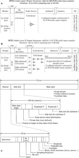
FIGURE 11.1 Structure of the MPEG-1 audio Layer I, II, and III bitstreams. The header and some other fields are common, but other fields differ. Higher-level codecs can transcode lower-level bitstreams. A. Layer I bitstream format. B. Layer II bitstream format. C. Layer III bitstream format.

MPEG-1 Layer I

The MPEG-1 Layer I codec is a simplified version of the MUSICAM codec. It is a subband codec, designed to provide high fidelity with low complexity, but at a high bit rate. Block diagrams of a Layer I encoder and decoder (which also applies to Layer II) are shown in Fig. 11.2. A polyphase filter splits the wideband signal into 32 subbands of equal width. The filter is critically sampled; there is the same number of samples in the analyzed domain as in the time domain. Adjacent subbands overlap; a single frequency can affect two subbands. The filter and its inverse are not lossless; however, the error is small. The filter bank bands are all equal width, but the ear’s critical bands are not; this is compensated for in the bit allocation algorithm. For example, lower bands are usually assigned more bits, increasing their resolution over higher bands. This polyphase filter bank with 32 subbands is used in all three layers; Layer III adds additional hybrid processing.

The filter bank outputs 32 samples, one sample per band, for every 32 input samples. In Layer I, 12 subband samples from each of the 32 subbands are grouped to form a frame; this represents 384 wideband samples. At a 48-kHz sampling frequency, this comprises a block of 8 ms. Each subband group of 12 samples is given a bit allocation; subbands judged inaudible are given a zero allocation. Based on the calculated masking threshold (just audible noise), the bit allocation determines the number of bits used to quantize those samples. A floating-point notation is used to code samples; the mantissa determines resolution and the exponent determines dynamic range. A fixed scale factor exponent is computed for each subband with a nonzero allocation; it is based on the largest sample value in the subband. Each of the 12 subband samples in a block is normalized by dividing it by the same scale factor; this optimizes quantizer resolution.

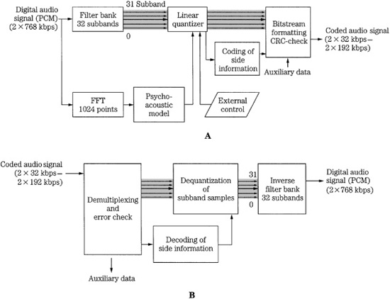
FIGURE 11.2 MPEG-1 Layer I or II audio encoder and decoder. The 32-subband filter bank is common to all three layers. A. Layer I or II encoder (single-channel mode). B. Layer I or II two-channel decoder.

A 512-sample FFT wideband transform located in a side chain performs spectral analysis on the audio signal. A psychoacoustic model, described in more detail later, uses a spreading function to emulate a basilar membrane response to establish masking contours and compute signal-to-mask ratios. Tonal and nontonal (noise-like) signals are distinguished. The psychoacoustic model compares the data to the minimum threshold curve. Using scale factor information, normalized samples are quantized by the bit allocator to achieve data reduction. The subband data is coded, not the FFT spectra.

Dynamic bit allocation assigns mantissa bits to the samples in each coded subband, or omits coding for inaudible subbands. Each sample is coded with one PCM codeword; the quantizer provides 2ⁿ−1 steps where 2 ≤ n ≤ 15. Subbands with a large signal-to-mask ratio are iteratively given more bits; subbands with a small SMR value are given fewer bits. In other words, the SMR determines the minimum signal-to-noise ratio that has to be met by the quantization of the subband samples. Quantization is performed iteratively. When available, additional bits are added to codewords to increase the signal-to-noise ratio (SNR) value above the minimum. Because the long block size might expose quantization noise in a transient signal, coarse quantization is avoided in blocks of low-level audio that are adjacent to blocks of high-level (transient) audio. The block scale factor exponent and sample mantissas are output. Error correction and other information are added to the signal at the output of the codec.

Playback is accomplished by decoding the bit allocation information, and decoding the scale factors. Samples are requantized by multiplying them with the correct scale factor. The scale factors provide all the information needed to recalculate the masking thresholds. In other words, the decoder does not need a psychoacoustic model. Samples are applied to an inverse synthesis filter such that subbands are placed at the proper frequency and added, and the resulting broadband audio waveform is output in consecutive blocks of thirty-two 16-bit PCM samples.

Example of MPEG-1 Layer I Implementation

As with other perceptual coding methods, MPEG-1 Layer I uses the ear’s audiology performance as its guide for audio encoding, relying on principles such as amplitude masking to encode a signal that is perceptually identical. Generally, Layer I operating at 384 kbps achieves the same quality as a Layer II codec operating at 256 kbps. Also, Layer I can be transcoded to Layer II. The following describes a simple Layer I implementation without a psychoacoustic model; its design is basic compared to other modern codecs.

PCM data with 32-, 44.1-, or 48-kHz sampling frequencies can be input to an encoder. At these three sampling frequencies, the subband width is 500, 689, and 750 Hz, and the frame period is 12, 8.7, and 8 ms, respectively. The following description assumes a 48-kHz sampling frequency. The stereo audio signal is passed to the first stage in a Layer I encoder, as shown in Fig. 11.3. A 24-bit finite impulse response (FIR) filter with the equivalent of 512 taps divides the audio band into 32 subbands of equal 750-Hz width. The filter window is shifted by 32 samples each time (12 shifts) so all the 384 samples in the 8-ms frame are analyzed. The filter bank outputs 32 subbands. With this filter, the effective sampling frequency of a subband is reduced by 32 to 1, for example, from a frequency of 48 kHz to 1.5 kHz. Although the channels are bandlimited, they are still in PCM representation at this point in the algorithm. The subbands are equal width, whereas the ear’s critical bands are not. This can be compensated for by unequally allocating bits to the subbands; more bits are typically allocated to code signals in lower-frequency subbands.

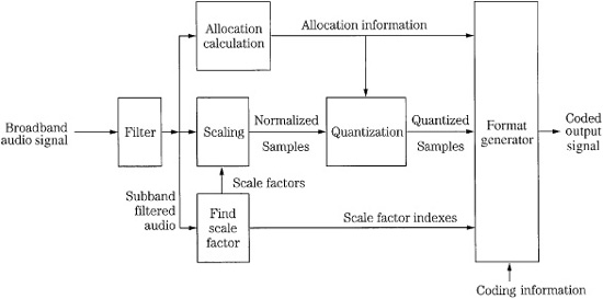
FIGURE 11.3 Example of an MPEG-1 Layer I encoder. The FFT side chain is omitted.

The encoder analyzes the energy in each subband to determine which subbands contain audible information. This example of a Layer I encoder does not use an FFT side chain or psychoacoustic model. The algorithm calculates average power levels in each subband over the 8-ms (12-sample) period. Masking levels in subbands and adjacent subbands are estimated. Minimum threshold levels are applied. Peak power levels in each subband are calculated and compared to masking levels. The SMR value (difference between the maximum signal and the masking threshold) is calculated for each sub-band and is used to determine the number of bits N assigned to a subband (i) such that N_i ≥ (SMR_i−1.76)/6.02. A bit pool approach is taken to optimally code signals within the given bit rate. Quantized values form a mantissa, with a possible range of 2 to 15 bits. Thus, a maximum resolution of 92 dB is available from this part of the coding word. In practice, in addition to signal strength, mantissa values also are affected by rate of change of the waveform pattern and available data capacity. In any event, new mantissa values are calculated for every sample period.

Audio samples are normalized (scaled) to optimally use the dynamic range of the quantizer. Specifically, six exponent bits form a scale factor, which is determined by the signal’s largest absolute amplitude in a block. The scale factor acts as a multiplier to optimally adjust the gain of the samples for quantization. This scale factor covers the range from −118 dB to + 6 dB in 2-dB steps. Because the audio signal varies slowly in relation to the sampling frequency, the masking threshold and scale factors are calculated only once for every group of 12 samples, forming a frame (12 samples/subband × 32 subbands = 384 samples). For every subband, the absolute peak value of the 12 samples is compared to a table of scale factors, and the closest (next highest) constant is applied. The other sample values are normalized to that factor, and during decoding will be used as multipliers to compute the correct subband signal level.

A floating-point representation is used. One field contains a fixed-length 6-bit exponent, and another field contains a variable length 2- to 15-bit mantissa. Every block of 12 subband samples may have different mantissa lengths and values, but would share the same exponent. Allocation information detailing the length of a mantissa is placed in a 4-bit field in each frame. Because the total number of bits representing each sample within a subband is constant, this allocation information (like the exponent) needs to be transmitted only once every 12 samples. A null allocation value is conveyed when a subband is not encoded; in this case neither exponent nor mantissa values within that subband are transmitted. The 15-bit mantissa yields a maximum signal-to-noise ratio of 92 dB. The 6-bit exponent can convey 64 values. However, a pattern of all 1’s is not used, and another value is used as a reference. There are thus 62 values, each representing 2-dB steps for an ideal total of 124 dB. The reference is used to divide this into two ranges, one from 0 to −118 dB, and the other from 0 to + 6 dB. The 6 dB of headroom is needed because a component in a single subband might have a peak amplitude 6 dB higher than the broadband composite audio signal. In this example, the broadband dynamic range is thus equivalent to 19 bits of linear coding.

A complete frame contains synchronization information, sample bits, scale factors, bit allocation information, and control bits for sampling frequency information, emphasis, and so on. The total number of bits in a frame (with two channels, with 384 samples, over 8 ms, sampled at 48 kHz) is 3072. This in turn yields a 384-kbps bit rate. With the addition of error detection and correction code, and modulation, the transmission bit rate might be 768 kbps. The first set of subband samples in a frame is calculated from 512 samples by the 512-tap filter and the filter window is shifted by 32 samples each time into 11 more positions during a frame period. Thus, each frame incorporates information from 864 broadband audio samples per channel.

Sampling frequencies of 32 kHz and 44.1 kHz also are supported, and because the number of bands remains fixed at 32, the subband width becomes 689.06 Hz with a 44.1-kHz sampling frequency. In some applications, because the output bit rate is fixed at 384 kbps, and 384 samples/channel per frame is fixed, there is a reduction in frame rate at sampling frequencies of 32 kHz and 44.1 kHz, and thus an increase in the number of bits per frame. These additional bits per frame are used by the algorithm to further increase audio quality.

Layer I decoding proceeds frame by frame, using the processing shown in Fig. 11.4. Data is reformatted to PCM by a subband decoder, using allocation information and scale factors. Received scale factors are placed in an array with two columns of 32 rows, each six bits wide. Each column represents an output channel, and each row represents one subband. The decoded subband samples are multiplied by their scale factors to restore them to their quantized values; empty subbands are automatically assigned a zero value. A synthesis reconstruction filter recombines the 32 subbands into one broadband audio signal. This subband filter operates identically (but inversely) to the input filter. As in the encoder, 384 samples/channel represent 8 ms of audio signal (at a sampling frequency of 48 kHz). Following this subband filtering, the signal is ready for reproduction through D/A converters.

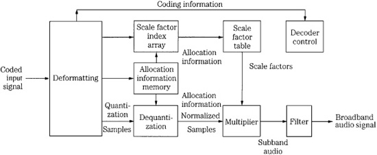
FIGURE 11.4 Example of an MPEG-1 Layer I decoder.

Because psychoacoustic processing, bit allocation, and other operations are not used in the decoder, its cost is quite low. Also, the decoder is transparent to improvements in encoder technology. If encoders are improved, the resulting fidelity would improve as well. Because the encoding algorithm is a function of digital signal processing, more sophisticated coding is possible. For example, because the number of bits per frame varies according to sampling rate, it might be expedient to create different allocation tables for different sampling frequencies.

An FFT side chain would permit analysis of the spectral content of subbands and psychoacoustic modeling. For example, knowledge of where signals are placed within bands can be useful in more precisely assigning masking curves to adjacent bands. The encoding algorithm might assume signals are at band edges, the most conservative approach. Such an encoder might claim 18-bit performance. Subjectively, at a 384-kbps bit rate, most listeners are unable to differentiate between a simple Layer I recording and an original CD recording.

MPEG-1 Layer II

The MPEG-1 Layer II codec is essentially identical to the original MUSICAM codec (the frame headers differ). It is thus similar to Layer I, but is more sophisticated in design. It provides high fidelity with somewhat higher complexity, at moderate bit rates. It is a sub-band codec. Figure 11.5 gives a more detailed look at a Layer II encoder (which also applies to Layer I). The filter bank creates 32 equal-width subbands, but the frame size is tripled to 3 × 12 × 32, corresponding to 1152 wideband samples per channel. In other words, data is coded in three groups of 12 samples for each subband (Layer I uses one group). At a sampling frequency of 48 kHz, this comprises a 24-ms period. Figure 11.6 shows details of the subband filter bank calculation. The FFT analysis block size is increased to 1024 points. In Layer II (and Layer III) the psychoacoustic model performs two 1024-sample calculations for each 1152-sample frame, centering the first half and the second half of the frame, respectively. The results are compared and the values with the lower masking thresholds (higher SMR) in each band are used. Tonal (sinusoidal) and nontonal (noise-like) components are distinguished to determine their effect on the masking threshold.

A single bit allocation is given to each group of 12 subband samples. Up to three scale factors are calculated for each subband, each corresponding to a group of 12 sub-band samples and each representing a 2-dB step-size difference. However, to reduce the scale factor bit rate, the codec analyzes scale factors in three successive blocks in each subband. When differences are small or when temporal masking will occur, one scale factor can be shared between groups. When transient audio content is coded, two or three scale factors can be conveyed. Bit allocation is used to maximize both the subband and frame signal-to-mask ratios. Quantization covers a range from 3 to 65,535 (or none), but the number of available levels depends on the subband. Low-frequency subbands can receive as many as 15 bits, middle-frequency subbands can receive seven bits, and high-frequency subbands are limited to three bits. In each band, prominent signals are given longer codewords. It is recognized that quantization varies with subband number; higher subbands usually receive fewer bits, with larger step sizes. Thus for greater efficiency, three successive samples (for all 32 subbands) are grouped to form a granule and quantized together.

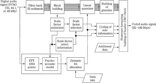
FIGURE 11.5 MPEG-1 Layer II audio encoder (single-channel mode) showing scale factor selection and coding of side information.

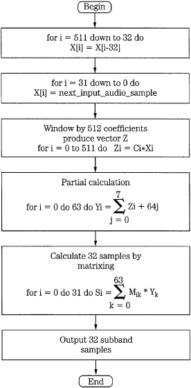
FIGURE 11.6 Flow chart of the analysis filter bank used in the MPEG-1 audio standard.

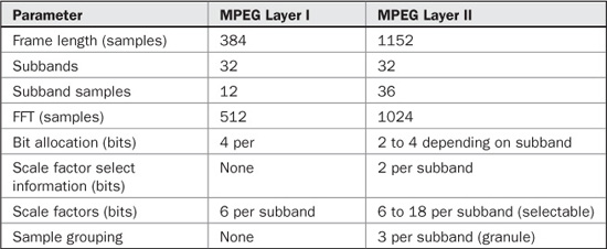
TABLE 11.1 Comparison of parameters in MPEG-1 Layer I and Layer II.

As in Layer I, decoding is relatively simple. The decoder unpacks the data frames and applies appropriate data to the reconstruction filter. Layer II coding can use stereo intensity coding. Layer II coding provides for a dynamic range control to adapt to different listening conditions, and uses a fixed-length data word. Minimum encoding and decoding delays are about 30 ms and 10 ms, respectively. Layer II is used in some digital audio broadcasting (DAB) and digital video broadcasting (DVB) applications. Layer I and II are compared in Table 11.1. Figure 11.7 shows a flow chart summarizing the complete MPEG-1 Layer I and II encoding algorithm.

MPEG-1 Layer III (MP3)

The MPEG-1 Layer III codec is based on the ASPEC codec and contains elements of MUSICAM, such as a subband filter bank, to provide compatibility with Layers I and II. Unlike the Layer I and II codecs, the Layer III codec is a transform codec. Its design is more complex than the other layer codecs. Its strength is moderate fidelity even at low data rates. Layer III files are popularly known as MP3 files. Block diagrams of a Layer III encoder and decoder are shown in Fig. 11.8.

As in Layers I and II, a wideband block of 1152 samples is first split into 32 subbands with a polyphase filter; this provides backward compatibility with Layers I and II. Each subband’s contents are transformed into spectral coefficients by either a 6- or 18-point modified discrete cosine transform (MDCT) with 50% overlap (using a sine window) so that windows contain either 12 or 36 subband samples. The MDCT outputs a maximum of 32 × 18 = 576 spectral lines. The spectral lines are grouped into scale factor bands that emulate critical bands. At lower sampling frequencies optionally provided by MPEG-2, the frequency resolution is increased by a factor of two; at a 24-kHz sampling rate the resolution per spectral line is about 21 Hz. This allows better adaptation of scale factor bands to critical bands. This helps achieve good audio quality at lower bit rates.

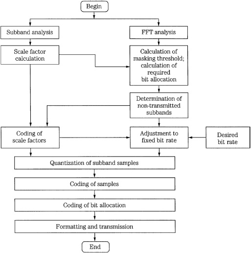
FIGURE 11.7 Flow chart of the entire MPEG-1 Layer I and II audio encoding algorithm.

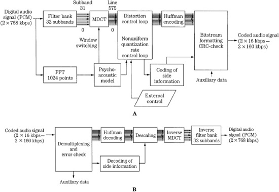
FIGURE 11.8 MPEG-1 Layer III audio encoder and decoder. A. Layer III encoder (single-channel mode). B. Layer III two-channel decoder.

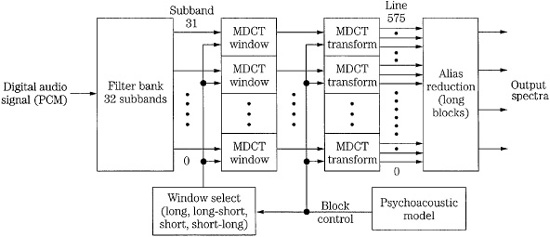
FIGURE 11.9 Long and short blocks can be selected for the MDCT transform used in the MPEG-1 Layer III encoder. Both long and short windows, and two transitional windows, are used.

Layer III has high frequency resolution, but this dictates low time resolution. Quantization error spread over a window length can produce pre-echo artifacts. Thus, under direction of the psychoacoustic model, the MDCT window sizes can be switched between frequency or time resolution, using a threshold calculation; the architecture is shown in Fig. 11.9. A long symmetrical window is used for steady-state signals; a length of 1152 samples corresponds 24 ms at a 48-kHz sampling frequency. Each transform of 36 samples yields 18 spectral coefficients for each of 32 subbands, for a total of 576 coefficients. This provides good spectral resolution of 41.66 Hz (24000/576) that is needed for steady state-signals, at the expense of temporal resolution that is needed for transient signals.

Alternatively, when transient signals occur, a short symmetrical window is used with one-third the length of the long window, followed by an MDCT that is one-third length. Time resolution is 4 ms at a 48-kHz sampling frequency. Three short windows replace one long window, maintaining the same number of samples in a frame. This mode yields six coefficients per subband, or a total of 32 × 6 = 192 coefficients. Window length can be independently switched for each subband. Because the switchover is not instantaneous, an asymmetrical start window is used to switch from long to short windows, and an asymmetrical stop window switches back. This ensures alias cancellation. The four window types, along with a typical window sequence, are shown in Fig. 11.10. There are three block modes. In two modes, the outputs of all 32 subbands are processed through the MDCT with equal block lengths. A mixed mode provides frequency resolution at lower frequencies and time resolution at higher frequencies. During transients, the two lower subbands use long blocks and the upper 30 subbands use short blocks. Huffman coding is applied at the encoder output to additionally lower the bit rate.

A Layer III decoder performs Huffman decoding, as well as decoding of bit allocation information. Coefficients are applied to an inverse transform, and 32 subbands are combined in a synthesis filter to output a broadband signal. The inverse modified discrete cosine transform (IMDCT) is executed 32 times for 18 spectral values each to transform the spectrum of 576 values into 18 consecutive spectra of length 32. These spectra are converted into the time domain by executing a polyphase synthesis filter bank 18 times. The polyphase filter bank contains a frequency mapping operation (such as matrix multiplication) and an FIR filter with 512 coefficients.

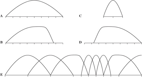
FIGURE 11.10 MPEG-1 Layer III allows adaptive window switching for the MDCT transform. Four window types are defined. A. Long (normal) window. B. Start window (long to short). C. Short window. D. Stop window (short to long). D. An example of a window sequence. (Brandenburg and Stoll, 1994)

MP3 files can be coded at a variety of bit rates. However, the format is not scalable with respect to variable decoding. In other words, the decoder cannot selectively choose subsets of the entire bitstream to reproduce different quality signals.

MP3 Bit Allocation and Huffman Coding

The allocation control algorithm suggested for the Layer III encoder uses dynamic quantization. A noise allocation iteration loop is used to calculate optimal quantization noise in each subband. This technique is referred to as noise allocation, as opposed to bit allocation. Rather than allocate bits directly from SNR values, in noise allocation the bit assignment is an inherent outcome of the strategy. For example, an analysis-by-synthesis method can be used to calculate a quantized spectrum that satisfies the noise requirements of the modeled masking threshold. Quantization of this spectrum is iteratively adjusted so the bit rate limits are observed. Two nested iteration loops are used to find two values that are used in the allocation: the global gain value determines quantization step size, and scale factors determine noise-shaping factors for each scale factor band. To form scale factors, most of the 576 spectral lines in long windows are grouped into 21 scale factor bands, and most of the 192 lines from short windows are grouped into 12 scale factor bands. The grouping approximates critical bands, and varies according to sampling frequency.

An inner iteration loop (called the rate loop) acts to decrease the coder rate until it is sufficiently low. The Huffman code assigns shorter codewords to smaller quantized values that occur more frequently. If the resulting bit rate is too high, the rate loop adjusts gain to yield larger quantization step sizes and hence small quantized values and smaller Huffman codewords and a lower bit rate. The process of quantizing spectral lines and determining the appropriate Huffman code can be time-consuming. The outer iteration loop (called the noise control loop) uses analysis-by-synthesis to evaluate quantization noise levels and hence the quality of the coded signal. The outer loop decreases the quantizer step size to shape the quantization noise that will appear in the reconstructed signal, aiming to maintain it below the masking threshold in each band. This is done by iteratively increasing scale factor values. The algorithm uses the iterative values to compute the resulting quantization noise. If the quantization noise level in a band exceeds the masking threshold, the scale factor is adjusted to decrease the step size and lower the noise floor. The algorithm then recalculates the quantization noise level. Ideally, the loops yield values such that the difference between the original spectral values and the quantized values results in noise below the masking threshold.

If the psychoacoustic model demands small step sizes and in contradiction the loops demand larger step sizes to meet a bit rate, the loops are terminated. To avoid this, the perceptual model can be modified and two loops tuned, to suit different bit rates; this tuning can require considerable development work. Nonuniform quantization is used such that step size varies with amplitude. Values are raised to the 3/4 power before quantizing to optimize the signal-to-noise ratio over a range of quantizer values (the decoder reciprocates by raising values to the 4/3 power).

Huffman and run-length entropy coding exploit the statistical properties of the audio signal to achieve lossless data compression. Most audio frames will yield larger spectral values at low frequencies and smaller (or zero) values at higher frequencies. To utilize this, the 576 spectral lines are considered as three groups and can be coded with different Huffman code tables. The sections from low to high frequency are BIG_ VALUE, COUNT1, and RZERO, assigned according to pairs of absolute values ranging from 0 to 8191, quadruples of 0, −1, or + 1 values, and the pairs of 0 values, respectively. The BIG_VALUE pairs can be coded using any of 32 Huffman tables, and the COUNT1 quadruples can be coded with either of two tables. The RZERO pairs are not coded with Huffman coding. A Huffman table is selected based on the dynamic range of the values. Huffman coding is used for both scale factors and coefficients.

The data rate from frame to frame can vary in Layer III; this can be used for variable bit-rate recording. The psychoacoustic model calculates how many bits are needed and sets the frame bit rate accordingly. In this way, for example, music passages that can be satisfactorily coded with fewer bits can yield frames with fewer bits. A variable bit rate is efficient for on-demand transmission. However, variable bit rate streams cannot be transmitted in real time using systems with a constant bit rate. When a constant rate is required, Layer III can use an optional bit reservoir to allow for more accurate coding of particularly difficult (large perceptual entropy) short window passages. In this way, the average transmitted data rate can be smaller than peak data rates. The number of bits per frame is variable, but has a constant long-term average. The mean bit rate is never allowed to exceed the fixed-channel capacity. In other words, there is reserve capacity in the reservoir. Unneeded bits (below the average) can be placed in the reservoir. When additional bits are needed (above the average), they are taken from the reservoir. Succeeding frames are coded with somewhat fewer bits than average to replenish the reservoir. Bits can only be borrowed from past frames; bits cannot be borrowed from future frames. The buffer memory adds throughput time to the codec. To achieve synchronization at the decoder, headers and side information are conveyed at the frame rate. Frame size is variable; boundaries of main data blocks can vary whereas the frame headers are at fixed locations. Each frame has a synchronization pattern and subsequent side information discloses where a main data block began in the frame. In this way, main data blocks can be interrupted by frame headers.

In some codecs, the output file size is different from the input file size, and the signals are not time-aligned; the time duration of the codec’s signal is usually longer. This is because of the block structure of the processing, coding delays, and the lookahead strategies employed. Moreover, for example, an encoder might either discard a final frame that is not completely filled at the end of a file, or more typically pad the last frame with zeros. To maintain the original file size and time alignment, some codecs use ancillary data in the bitstream in a technique known as original file length (OFL). By specifying the number of samples to be stripped at the start of a file, and the length of the original file, the number of samples to be stripped at the end can be calculated. The OFL feature is available in the MP3PRO codec.

MP3 Stereo Coding

To take advantage of redundancies between stereo channels, and to exploit limitations in human spatial listening, Layer III allows a choice of stereo coding methods, with four basic modes: normal stereo mode with independent left and right channels; M/S stereo mode in which the entire spectrum is coded with M/S; intensity stereo mode in which the lower spectral range is coded as left/right and the upper spectral range is coded as intensity; and the intensity and M/S mode in which the lower spectral range is coded as M/S and the upper spectral range is coded as intensity. Each frame may have a different mode. The partition between upper and lower spectral modes can be changed dynamically in units of scale factor bands.

Layer III supports both M/S (middle/side) stereo coding and intensity stereo coding. In M/S coding, certain frequency ranges of the left and right channels are mixed as sum (middle) and difference (side) signals of the left and right channels before quantization. In this way, stereo unmasking can be avoided. In addition, when there is high correlation between the left and right channels, the difference signal is further reduced to conserve bits. In intensity stereo coding, the left and right channels of upper-frequency subbands are not coded individually. Instead, one summed signal is transmitted along with individual left- and right-channel scale factors indicating position in the stereo panorama. This method retains one spectral shape for both channels in upper sub-bands, but scales the magnitudes. This is effective for stationary signals, but less effective for transient signals because they may have different envelopes in different channels. Intensity coding may lead to artifacts such as changes in stereo imaging, particularly for transient signals. It is used primarily at low bit rates.

MP3 Decoder Optimization

MP3 files can be decoded with dedicated hardware chips or software programs. To optimize operation and decrease computation, some software decoders implement special features. Calculation of the hybrid synthesis filter bank is the most computationally complex aspect of the decoder. The process can be simplified by implementing a stereo downmix to monaural in the frequency domain, before the filter bank, so that only one filter operation must be performed. Downmixing can be accomplished with a simple weighted sum of the left and right channels. However, this is not optimal because, for example, an M/S-stereo or intensity-stereo signal already contains a sum signal. More efficiently, built in downmixing routines can calculate the sum signal only for those scale factor bands that are coded in left/right stereo. For M/S- and intensity-coded scale factor bands, only scaling operations are needed.

To further reduce computational complexity, the hybrid filter bank can be optimized. The filter bank consists of IMDCT and polyphase filter bank sections. As noted, the IMDCT is executed 32 times for 18 spectral values each to transform the spectrum of 576 values into 18 consecutive spectra of length 32. These spectra are converted into the time domain by executing a polyphase synthesis filter bank 18 times. The polyphase filter bank contains a frequency mapping operation (such as matrix multiplication) and a FIR filter with 512 coefficients. The FIR filter calculation can be simplified by reducing the number of coefficients, the filter coefficients can be truncated at the ends of the impulse response, and the impulse response can be modeled with fewer coefficients. Experiments have suggested that filter length can be reduced by 25% without yielding additional audible artifacts. More directly, computation can be reduced by limiting the output audio bandwidth. The high-frequency spectral values can be set to zero; an IMDCT with all input samples set to zero does not have to be calculated. If only the lower halves of the IMDCTs are calculated, the audio bandwidth is limited. The output can be downsampled by a factor of 2, so that computation for every second output value can be skipped, thus cutting the FIR calculation in half.

There are many nonstandard codecs that produce MP3-compliant bitstreams; they vary greatly in performance quality. LAME is an example of a fast, high-quality, royalty-free codec that produces a MP3-compliant bitstream. LAME is open-source, but using LAME may require a patent license in some countries. LAME is available at http://lame.sourceforge.net. MP3 Internet applications are discussed in Chap. 15.

MPEG-1 Psychoacoustic Model 1

The MPEG-1 standard suggests two psychoacoustic models that determine the minimum masking threshold for inaudibility. The models are only informative in the standard; their use is not mandated. The models are used only in the encoder. In both cases, the difference between the maximum signal level and the masking threshold is used by the bit allocator to set the quantization levels. Generally, model 1 is applied to Layers I and II and model 2 is applied to Layer III.

Psychoacoustic model 1 proposes a low-complexity method to analyze spectral data and output signal-to-mask ratios. Model 1 performs these nine steps:

1. Perform FFT analysis: A 512- or 1024-point fast Fourier transform, with a Hann window with adjacent overlapping of 32 or 64 samples, respectively, to reduce edge effects, is used to transform time-aligned time-domain data to the frequency domain. An appropriate delay is applied to time-align the psychoacoustic model’s output. The signal is normalized to a maximum value of 96 dB SPL, calibrating the signal’s minimum value to the absolute threshold of hearing.

2. Determine the sound pressure level: The maximum SPL is calculated for each subband by choosing the greater of the maximum amplitude spectral line in the subband or the maximum scale factor that accounts for low-level spectral lines in the subband.

3. Consider the threshold in quiet: An absolute hearing threshold in the absence of any signal is given; this forms the lower masking bound. An offset is applied depending on the bit rate.

4. Finding tonal and nontonal components: Tonal (sinusoidal) and nontonal (noise-like) components in the signal are identified. First, local maxima in the spectral components are identified relative to bandwidths of varying size. Components that are locally prominent in a critical band by + 7 dB are labeled as tonal and their sound-pressure level is calculated. Intensities of the remaining components, assumed to be nontonal, within each critical band are summed and their SPL is calculated for each critical band. The nontonal maskers are centered in each critical band.

5. Decimation of tonal and nontonal masking components: The number of maskers is reduced to obtain only the relevant maskers. Relevant maskers are those with magnitude that exceeds the threshold in quiet, and those tonal components that are strongest within 1/2 Bark.

6. Calculate individual masking thresholds: The total number of masker frequency bins is reduced (for example, in Layer I at 48 kHz, 256 is reduced to 102) and maskers are relocated. Noise masking thresholds for each subband, accounting for tonal and nontonal components and their different downward shifts, are determined by applying a masking (spreading) function to the signal. Calculations use a masking index and masking function to describe masking effects on adjacent frequencies. The masking index is an attenuation factor based on critical-band rate. The piecewise masking function is an attenuation factor with different lower and upper slopes between −3 and + 8 Bark that vary with respect to the distance to the masking component and the component’s magnitude. When the subband is wide compared to the critical band, the spectral model can select a minimum threshold; when it is narrow, the model averages the thresholds covering the subband.

7. Calculate the global masking threshold: The powers corresponding to the upper and lower slopes of individual subband masking curves, as well as a given threshold of hearing (threshold in quiet), are summed to form a composite global masking contour. The final global masking threshold is thus a signal-dependent modification of the absolute threshold of hearing as affected by tonal and nontonal masking components across the basilar membrane.

8. Determine the minimum masking threshold: The minimum masking level is calculated for each subband.

9. Calculate the signal-to-mask ratio: Signal-to-mask ratios are determined for each subband, based on the global masking threshold. The difference between the maximum SPL levels and the minimum masking threshold values determines the SMR value in each subband; this value is supplied to the bit allocator.

The principal steps in the operation of model 1 can be illustrated with a test signal that contains a band of noise, as well as prominent tonal components. The model analyzes one block of the 16-bit test signal sampled at 44.1 kHz. Figure 11.11A shows the audio signal as output by the FFT; the model has identified the local maxima. The figure also shows the absolute threshold of hearing used in this particular example (offset by −12 dB). Figure 11.11B shows tonal components marked with a “+” and nontonal components marked with a “o.” Figure 11.11C shows the masking functions assigned to tonal maskers after decimation. The peak SMR (about 14.5 dB) corresponds to that used for tonal maskers. Figure 11.11D shows the masking functions assigned to nontonal maskers after decimation. The peak SMR (about 5 dB) corresponds to that used for nontonal maskers. Figure 11.11E shows the final global masking curve obtained by combining the individual masking thresholds. The higher of the global masking curve and the absolute threshold of hearing is used as the final global masking curve. Figure 11.11F shows the minimum masking threshold. From this, SMR values can be calculated in each subband.

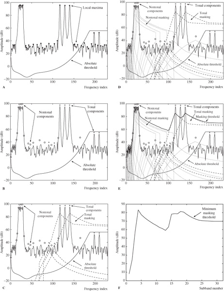
FIGURE 11.11 Operation of MPEG-1 model 1 is illustrated using a test signal. A. Local maxima and absolute threshold. B. Tonal and nontonal components. C. Tonal masking. D. Nontonal masking. E. Masking threshold. F. Minimum masking threshold.

To further explain the operation of model 1, additional comments are given here. The delay in the 512-point analysis filter bank is 256 samples and centering the data in the 512-point Hann window adds 64 samples. An offset of 320 samples (256 + (512 − 384)/2 = 320) is needed to time-align the model’s 384 samples.

The spreading function used in model 1 is described in terms of piecewise slopes (in dB):

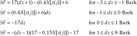
where dz = z(i) − z(j) is the distance in Bark between the maskee and masker frequency; i and j are index values of spectral lines of the maskee and masker, respectively. X[z(j)] is the sound pressure level of the jth masking component in dB. Values outside −3 and + 8 Bark are not considered in this model.

Model 1 uses this general approach to detect and characterize tonality in audio signals: An FFT is applied to 512 or 1024 samples, and the components of the spectrum analysis are considered. Local maxima in the spectrum are identified as having more energy than adjacent components. These components are decimated such that a tonal component closer than 1/2 Bark to a stronger tonal component is discarded. Tonal components below the threshold of hearing are discarded as well. The energies of groups of remaining components are summed to represent tonal components in the signal; other components are summed and marked as nontonal. A binary designation is given: tonal components are assigned 1, and nontonal components are assigned 0. This information is presented to the bit allocation algorithm. Specifically, in model 1, tonality is determined by detecting local maxima of 7 dB in the audio spectrum. To derive the masking threshold relative to the masker, a level shift is applied; the nature of the shift depends on whether the masker is tonal or nontonal:

Δ_T(z) = −6.025 − 0.275z dB

Δ_N(z) = −2.025 − 0.175z dB

where z is the frequency of the masker in Bark.

Model 1 considers all the nontonal components in a critical band and represents them with one value at one frequency. This is appropriate at low frequencies where sub-bands and critical bands have good correspondence, but can be inefficient at high frequencies where there are many critical bands in each subband. A subband that is apart from the identified nontonal component in a critical band may not receive a correct nontonal evaluation.

MPEG-1 Psychoacoustic Model 2

Psychoacoustic model 2 performs a more detailed analysis than model 1, at the expense of greater computational complexity. It is designed for lower bit rates than model 1. As in model 1, model 2 outputs a signal-to-mask ratio for each subband; however, its approach is significantly different. It contours the noise floor of the signal represented by many spectral coefficients in a way that is more accurate than that allowed by coarse subband coding. Also, the model uses an unpredictability measure to examine the side-chain data for tonal or nontonal qualities. Model 2 performs these 14 steps:

1. Reconstruct input samples: A set of 1024 input samples is assembled.

2. Calculate the complex spectrum: The time-aligned input signal is windowed with a 1024-point Hann window; alternatively, a shorter window may be used. An FFT is computed and output represented in magnitude and phase.

3. Calculate the predicted magnitude and phase: The predicted magnitude and phase are determined by extrapolation from the two preceding threshold blocks.

4. Calculate the unpredictability measure: The unpredictability measure is computed using the Euclidian distance between the predicted and actual values in the magnitude/phase domain. To reduce complexity, the measure may be computed only for lower frequencies and assumed constant for higher frequencies.

5. Calculate the energy and unpredictability in the partitions: The energy magnitude and the weighted unpredictability measure in each threshold calculation partition are calculated. A partition has a resolution of one spectral line (at low frequencies) or 1/3 critical band (at high frequencies), whichever is wider.

6. Convolve energy and unpredictability with the spreading function: The energy and the unpredictability measure in threshold calculation partitions are each convolved with a cochlea spreading function. Values are renormalized.

7. Derive tonality index: The unpredictability measures are converted to tonality indices ranging from 0 (high unpredictability) to 1 (low unpredictability). This determines the relative tonality of the maskers in each threshold calculation partition.

8. Calculate the required signal-to-noise ratio: An SNR is calculated for each threshold calculation partition using tonality to interpolate an attenuation shift factor between noise-masking-tone (NMT) and tone-masking-noise (TMN). The interpolated shift ranges from 5.5 dB for NMT and upward. The final shift value is the higher of the interpolated value or a frequency-dependent minimum value.

9. Calculate power ratio: The power ratio of the SNR is calculated for each threshold calculation partition.

10. Calculate energy threshold: The actual energy threshold is calculated for each threshold calculation partition.

11. Spread threshold energy: The masking threshold energy is spread over FFT lines corresponding to threshold calculation partitions to represent the masking in the frequency domain.

12. Calculate final energy threshold of audibility: The spread threshold energy is compared to values in absolute threshold of quiet tables, and the higher value is used (not the sum) as the energy threshold of audibility. This is because it is wasteful to specify a noise threshold lower than the level that can be heard.

13. Calculate pre-echo control: A narrow-band pre-echo control used in the Layer III encoder is calculated, to prevent audibility of the error signal spread in time by the synthesis filter. The calculation lowers the masking threshold after a quiet signal. The calculation takes the minimum of the comparison of the current threshold with the scaled thresholds of two previous blocks.

14. Calculate signal-to-mask ratios: Threshold calculation partitions are converted to codec partitions (scale factor bands). The SMR (energy in each scale factor band divided by noise level in each scale factor band) is calculated for each partition and expressed in decibels. The SMR values are forwarded to the allocation algorithm.

The principal steps in the operation of model 2 can be illustrated with a test signal that contains three prominent tonal components. The model analyzes a set of 1024 input samples of the 16-bit test signal sampled at 44.1 kHz. Figure 11.12A shows the magnitude of the audio signal as output by the FFT; the phase is also computed. Following prediction of magnitude and phase, the unpredictability measure is computed, as shown in Fig. 11.12B, using the Euclidian distance between the predicted and actual values in the magnitude/phase domain. When the measure equals 0, the current value is completely predicted. Figure 11.12C shows the energy magnitude in each partition and the spreading functions that are applied. Figure 11.12D shows the tonality index derived from the unpredictability measure; the tonality index ranges from 0 (high unpredictability and noise-like) to 1 (low unpredictability and tonal). Figure 11.12E shows the spread masking threshold energy in the frequency domain and the absolute threshold of quiet; the higher value is used to find the energy threshold of inaudibility. Figure 11.12F shows signal-to-mask ratios (energy in each scale factor band divided by noise level in each scale factor band) in codec partitions.

To further explain the operation of model 2, additional comments are given here. The spreading function used in model 2 is:

10 log₁₀ SF(dz) = 15.8111389 + 7.5(1.05dz + 0.474) − 17.5[1.0 +(1.05dz +0.474)²]^1/2+8 MIN[(1.05dz − 0.5)² − 2(1.05dz − 0.5),0] dB

where dz is the distance in Bark between the maskee and masker frequency.

The spectral flatness measure (SFM), devised by James Johnston, measures the average or global tonality of the segment. SFM is the ratio of the geometric mean of the power spectrum to its arithmetic mean. The value is converted to decibels and referenced to −60 dB to provide a coefficient of tonality ranging continuously from 0 (nontonal) to 1 (tonal). This coefficient can be used to interpolate between TMN and NMT models. SFM leads to very conservative masking decisions for nontonal parts of a signal. More efficiently, specific tonal and nontonal regions within a segment can be identified. This local tonality can be measured as the normalized Euclidean distance between the actual and predicted values over two successive segments, for amplitude and phase. On the basis of this, tonality unpredictability can be computed for narrow frequency partitions and used to create tonality metrics that are used to interpolate between tone or noise models.

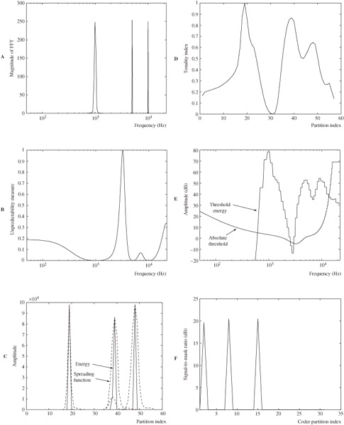
FIGURE 11.12 Operation of MPEG-1 model 2 is illustrated using a test signal. A. Magnitude of FFT. B. Unpredictability measure. C. Energy and spreading functions. D. Tonality index. E. Threshold energy and absolute threshold. F. Signal-to-mask ratios. (Boley and Rao, 2004)

Specifically, in model 2, a tonality index is created, on the basis of the predictability of the audio signal’s spectral components in a partition in two successive frames. Tonal components are more accurately predicted. Amplitude and phase are predicted to form an unpredictability measure C. When C = 0, the current value is completely predicted, and when C = 1, the predicted values differ from the actual values. This yields the tonality index T ranging from 0 (high unpredictability and noise-like) to 1 (low unpredictability and tonal). For example, the audio signal’s strongly tonal and nontonal areas are evident in Fig. 11.12D. The tonality index is used to calculate a (z) shift, for example, interpolating values from 6 dB (nontonal) to 29 dB (tonal).

When used in a Layer III encoder, model 2 is modified. The model is executed twice, once with a long block and once with a short 256-sample block. These values are used in the unpredictability measure calculation. A slightly different spreading function is used. The NMT shift is changed to 6.0 dB and a fixed TMN shift of 29.0 dB is used. As noted, a pre-echo control is calculated. Perceptual entropy is calculated as the logarithm of the geometric mean of the normalized spectral energy in a partition. This predicts the minimum number of bits needed for transparency. High values are used to identify transient attacks, and thus to determine block size in the encoder. In addition, model 2 accepts the minimum masking threshold at low frequencies where there is good correspondence between subbands and critical bands, and it uses the average of the thresholds at higher frequencies where subbands are narrow compared to critical bands.

Much research has been done since the informative model 2 was published in the MPEG-1 standard. Thus, most practical encoders use models that offer better performance, even if they are based on the informative model. An encoder that follows the informative documentation literally will not provide good results compared to more sophisticated implementations.

MPEG-2 Audio Standard

The MPEG-2 audio standard was designed for applications ranging from Internet downloading to high-definition digital television (HDTV) transmission. It provides a backward-compatible path to multichannel sound and a low sampling frequency provision, as well as a non-backward-compatible multichannel format known as Advanced Audio Coding (AAC). The MPEG-2 audio standard encompasses the MPEG-1 audio standard of Layers I, II, and III, using the same encoding and decoding principles as MPEG-1. In many cases, the same layer algorithms developed for MPEG-1 applications are used for MPEG-2 applications. Multichannel MPEG-2 audio is backward compatible with MPEG-1. An MPEG-2 decoder will accept an MPEG-1 bitstream and an MPEG-1 decoder can derive a stereo signal from an MPEG-2 bitstream. However, MPEG-2 also permits use of incompatible audio codecs.

One part of the MPEG-2 standard provides multichannel sound at sampling frequencies of 32, 44.1, and 48 kHz. Because it is backward compatible to MPEG-1, it is designated as BC (backward compatible), that is, MPEG-2 BC. Clearly, because there is more redundancy between six channels than between two, greater coding efficiency is achieved. Overall, 5.1 channels can be successfully coded at rates from 384 kbps to 640 kbps. MPEG-2 also supports monaural and stereo coding at sampling frequencies of 16, 22.05, and 24 kHz, using Layers I, II, and III. The MPEG-1 and -2 audio coding family is shown in Fig. 11.13. The MPEG-2 audio standard was approved by the MPEG committee in November 1994 and is specified in ISO/IEC 13818-3.

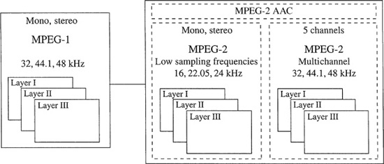
FIGURE 11.13 The MPEG-2 audio standard adds monaural/stereo coding at low sampling frequencies, multichannel coding, and AAC. The three MPEG-1 layers are supported.

The multichannel MPEG-2 BC format uses a five-channel approach sometimes referred to as 3/2 + 1 stereo (3 front and 2 surround channels + subwoofer). The low-frequency effects (LFE) subwoofer channel is optional, providing an audio range up to 120 Hz. A hierarchy of formats is created in which 3/2 may be downmixed to 3/1, 3/0, 2/2, 2/1, 2/0, and 1/0. The multichannel MPEG-2 BC format uses an encoder matrix that allows a two-channel decoder to decode a compatible two-channel signal that is a subset of a multichannel bitstream. The multiple channels of MPEG-2 are matrixed to form compatible MPEG-1 left/right channels, as well as other MPEG-2 channels, as shown in Fig. 11.14. The MPEG-1 left and right channels are replaced by matrixed MPEG-2 left and right channels and these are encoded into backward-compatible MPEG frames with an MPEG-1 encoder. Additional multichannel data is placed in the expanded ancillary data field.

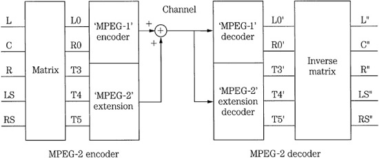
FIGURE 11.14 The MPEG-2 audio encoder and decoder showing how a 5.1-channel surround format can be achieved with backward compatibility with MPEG-1.

To efficiently code multiple channels, MPEG-2 BC uses techniques such as dynamic crosstalk reduction, adaptive interchannel prediction, and center channel phantom image coding. With dynamic crosstalk reduction, as with intensity coding, multichannel high-frequency information is combined and conveyed along with scale factors to direct levels to different playback channels. In adaptive prediction, a prediction error signal is conveyed for the center and surround channels. The high-frequency information in the center channel can be conveyed through the front left and right channels as a phantom image.

MPEG-2 BC can achieve a combined bit rate of 384 kbps, using Layer II at a 48-kHz sampling frequency. MPEG-2 allows for audio bit rates up to 1066 kbps. To accommodate this, the MPEG- 2 frame is divided into two parts. The first part is an MPEG-1-compatible stereo section with Layer I data up to 448 kbps, Layer II data up to 384 kbps, or Layer III data up to 320 kbps. The MPEG-2 extension part contains all other surround data.

A standard two-channel MPEG-1 decoder ignores the ancillary information, and reproduces the front main channels. In some cases, the dematrixing procedure in the decoder can yield an artifact in which the sound in a channel is mainly phase canceled but the quantization noise is not, and thus becomes audible. This limitation of spatial unmasking in MPEG-2 BC is a direct result of the matrixing used to achieve backward compatibility with the original two-channel MPEG standard. In part, it can be addressed by increasing the bit rate of the coded signals.

MPEG-2 also specifies Layer I, II, and III at low sampling frequencies (LSF) of 16, 22.05, and 24 kHz. This extension is not backward compatible to MPEG-1 codecs. This portion of the standard is known as MPEG-2 LSF. At these low bit rates, Layer III generally shows the best performance. Only minor changes in the MPEG-1 bit rate and bit allocation tables are necessary to adapt this LSF format. The relative improvement in quality stems from the improved frequency resolution of the polyphase filter bank in low- and mid-frequency regions; this allows more efficient application of masking. Layers I and II fare better than Layer III in these applications because Layer III already has good frequency resolution. The bitstream is unchanged in the LSF mode and the same frame format is used. For 24-kHz sampling, the frame length is 16 ms for Layer I and 48 ms for Layer II. The frame length of Layer III is decreased relative to that of MPEG-1. In addition, the “MPEG-2.5” standard supports sampling frequencies of 8, 11.025, and 12 kHz with the corresponding decrease in audio bandwidth; implementations use Layer III as the codec. Many MP3 codecs support the original MPEG-1 Layer III codec as well as the MPEG-2 and MPEG-2.5 extensions for lower sampling frequencies.

The menu of data rates, fidelity, and layer compatibility provided by MPEG are useful in a wide variety of applications such as computer multimedia, CD-ROM, DVD-Video, computer disks, local area networks, studio recording and editing, multichannel disk recording, ISDN transmission, digital audio broadcasting, and multichannel digital television. Numerous C and C++ programs performing MPEG-1 and -2 audio coding and decoding can be downloaded from a number of Internet file sites, and executed on personal computers. The backward-compatible format, using Layer II coding, is used for the soundtracks of some DVD-Video discs. However, a matrix approach to surround sound does not preserve spatial fidelity as well as discrete channel coding.

MPEG-2 AAC

The MPEG-2 Advanced Audio Coding (AAC) format codes monaural, stereo, or multi-channel playback for up to 48 channels, including 5.1-channel, at a variety of bit rates. AAC is known for its relatively high fidelity at low bit rates; for example, about 64 kbps per channel. It also provides high-quality 5.1-channel coding at an overall rate of 320 kbps or 384 kbps. AAC uses a reference model (RM) structure in which a set of tools (modules) has defined interfaces and can be combined variously in three different profiles. Individual tools can be upgraded and used to replace older tools in the reference software. In addition, this modularity makes it easy to compare revisions against older versions. AAC also comprises the kernel of audio tools used in the MPEG-4 standard for coding high-quality audio. AAC also supports lossless coding. AAC is specified in Part 7 of the MPEG-2 standard (ISO/IEC 13818-7), which was finalized in April 1997.

MPEG-2 AAC coding is not backward compatible with MPEG-1 and was originally designated as NBC (non-backward compatible) coding. An AAC bitstream cannot be decoded by an MPEG-1-only decoder. By lifting the constraint of compatibility, better performance is achieved compared to MPEG-2 BC. MPEG-2 AAC supports standard sampling frequencies of 32, 44.1, and 48 kHz, as well as other rates from 8 kHz to 96 kHz, yielding maximum bit rates of 48 kbps and 576 kbps, respectively. Its input channel configurations are: 1/0 (monaural), 2/0 (two-channel stereo), different multichannel configurations up to 3/2 + 1, and provision for up to 48 channels. Matrixing is not used. Downmixing is supported. To improve error performance, the system is designed to maintain bitstream synchronization in the presence of bit errors, and error concealment is supported as well.

To allow flexibility in audio quality versus processing requirements, AAC coding modules are used to create three profiles: main profile, scalable sampling rate (SSR) profile, and low-complexity (LC) profile. The main profile employs the most sophisticated encoder using all the coding modules except preprocessing to yield the highest audio quality at any bit rate. A main profile decoder can also decode the low-complexity bitstream. The SSR profile uses a gain control tool to perform poly-phase quadrature filtering (PQF), gain detection, and gain modification preprocessing; prediction is not used and temporal noise shaping (TNS) order is limited. SSR divides the audio signal into four equal frequency bands each with an independent bitstream and decoders can choose to decode one or more streams and thus vary the bandwidth of the output signal. SSR provides partial compatibility with the low-complexity profile; the decoded signal is bandlimited. The LC profile does not use preprocessing or prediction tools and the TNS order is limited. LC operates with low memory and processing requirements.

AAC Main Profile

A block diagram of a main profile AAC encoder and decoder is shown in Fig. 11.15. An MDCT with 50% overlap is used as the only input signal filter bank. It uses lengths of 1024 for stationary signals or 128 for transient signals, with a 2048-point window or a block of eight 256-point windows, respectively. To preserve interchannel block synchronization (phase), short block lengths are retained for eight-block durations. For multi-channel coding, different filter bank resolutions can be used for different channels. At 48 kHz, the long-window frequency resolution is 23 Hz and time resolution is 21 ms; the short window yields 187 Hz and 2.6 ms. The MDCT employs time-domain aliasing cancellation (TDAC). Two alternate window shapes are selectable on a frame basis in the 2048-point mode; either sine or Kaiser–Bessel-derived (KBD) windows can be employed. The encoder can select the optimal window shape on the basis of signal characteristics. The sine window is used when perceptually important components are spaced closer than 140 Hz and narrow-band selectivity is more important than stop-band attenuation. The KBD window is used when components are spaced more than 220 Hz apart and stopband attenuation is needed. Window switching is seamless, even with the overlap-add sequence. The shape of the left half of each window must match the shape of the right half of the preceding window; a new window shape is thus introduced as a new right half.

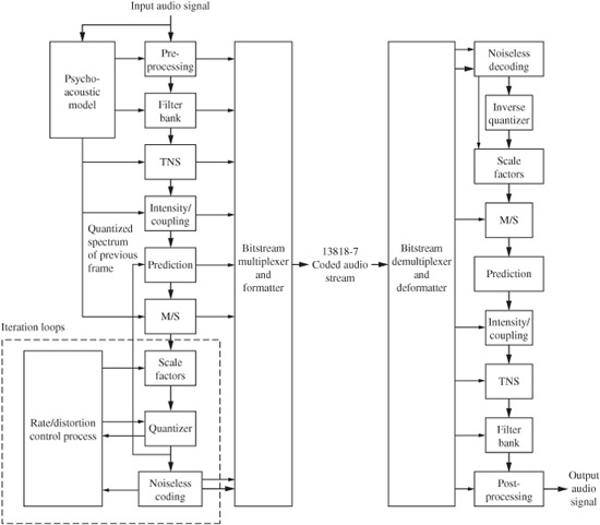
FIGURE 11.15 Block diagram of MPEG-2 AAC encoder and decoder. Heavy lines denote data paths, light lines denote control signals.

The suggested psychoacoustic model is based on the MPEG-1 model 2 and examines the perceptual entropy of the audio signal. It controls the quantizer step size, increasing step size to decrease buffer levels during stationary signals, and correspondingly decreasing step size to allow levels to rise during transient signals.

A second-order backward-adaptive predictor is applied to remove redundancy in stationary signals found in long windows; residues are calculated and used to replace frequency coefficients. Reconstructed coefficients in successive blocks are examined for frequencies below 16 kHz. Values from two previous blocks are used to form one predicted value for each current coefficient. The predicted value is subtracted from the actual target value to yield a prediction error (residue) which is quantized. Coefficient residues are grouped into scale factor bands that emulate critical bands. A prediction control algorithm determines if prediction should be activated in individual scale factor bands or in the frame at all, based on whether it improves coding gain.

AAC Allocation Loops

Two nested inner and outer loops iteratively perform nonuniform quantization and analysis-by-synthesis. The simplified nested algorithms are shown in Fig. 11.16. The inner loop (within the outer loop) begins with an initial quantization step size that is used to quantize the data and perform Huffman coding to determine the number of bits needed for coding. If necessary, the quantizer step size can be increased to reduce the number of bits needed. The outer loop uses scale factors to amplify scale factor bands to reduce audibility of quantization noise (inverse scale factors are applied in the decoder). Each scale factor band is assigned one multiplying scale factor. The scale factor is a gain value that changes the amplitude of the coefficients in the scale factor band; this shapes the quantization noise according to the masking threshold. The outer loop uses analysis-by-synthesis to determine the resulting distortion and this is compared to the distortion allowed by the psychoacoustic model; the best result so far is stored. If distortion is too high in a scale factor band, the band is amplified (this increases the bit rate) and the outer loop repeats. The two loops work in conjunction to optimally distribute quantization noise across the spectrum.

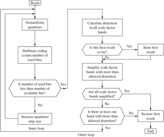
FIGURE 11.16 Two nested inner and outer allocation loops iteratively perform nonuniform quantization and analysis-by-synthesis.

The width of the scale factor bands is limited to 32 coefficients, except in the last scale factor band. There are 49 scale factor bands for long blocks. Scale factor bands can be individually amplified in increments of 1.5 dB. Noise shaping results because amplified coefficients have larger values and will yield a higher SNR after quantization. Because inverse amplification must be applied at the decoder, scale factors are transmitted in the bitstream. Designers should note that scale factors are defined with opposite polarity in MPEG-2 AAC and MPEG-1/2 Layer III (larger scale factor values represent larger signals in AAC, whereas it is the opposite in Layer III).

Huffman coding is applied to the quantized spectrum, scale factors, and directional information. Twelve Huffman codebooks are available to code pairs or quadruples of quantized spectral values. Two codebooks are available for each maximum value, each representing a different probability function. A bit reservoir accommodates instantaneously variable bit rates, allowing bits to be distributed across consecutive blocks for more effective coding within the average bit-rate constraint. A frame output consists of spectral coefficients and control parameters. The bitstream syntax defines a lower layer for raw audio data, and a higher layer contains audio transport data. In the decoder, current spectral components are reconstructed by adding a prediction error to the predicted value. As in the encoder, the coefficients are calculated from preceding values; no additional information is required.

AAC Temporal Noise Shaping

The spectral predictability of signals dictates the optimal coding strategy. For example, consider a steady-state sine wave comprising a flat temporal envelope, and a single spectral line—an impulse which is maximally nonflat spectrally. This sine wave is most easily coded directly in the frequency domain or by using linear prediction in the time domain. Conversely, consider a transient pulse signal comprising an impulse in the time domain, and a flat power spectrum. This pulse would be difficult to code directly in the frequency domain and difficult to code with prediction in the time domain. However, the pulse could be optimally coded directly in the time domain, or by using linear prediction in the frequency domain.

In the AAC codec, predictive coding is used to examine coefficients in each block. Transient signals will yield a more uniform spectrum and allow transients to be identified and more efficiently coded as residues. When coding transients, by analyzing the spectral data from the MDCT, temporal noise shaping (TNS) can be used to control the temporal shape of the quantization noise within each window to achieve perceptual noise shaping. By using the duality between the time and frequency domains, TNS provides improved predictive coding. When a time-domain signal is coded with predictive coding, the power spectral density of the quantization noise in the output signal will be shaped by the power spectral density of the input signal. Conversely, when a frequency-domain signal is coded with predictive coding, the temporal shape of the quantization noise in the output signal will follow the temporal shape of the input signal.

In particular, TNS shapes the temporal envelope of the quantization noise to follow the transient’s temporal envelope and thus conceals the noise under the transient. This can overcome problems such as pre-echo. As noted, this is accomplished with linear predictive coding of the spectral signal; for example, using open-loop differential pulse-code modulation (DPCM) encoding of spectral values. Corresponding DPCM decoding is performed in the decoder to create the output signal. During encoding, TNS replaces the target spectral coefficients with the forward-prediction residual (prediction error). In the AAC main profile, up to 20 successive coefficients in a block can be examined to predict the next coefficient and the prediction value is subtracted from the target coefficient to yield a spectral residue, which is quantized and encoded. A filter order up to 12 is allowed in the LC and SSR profiles. During decoding, the inverse predictive TNS filtering is performed to replace the residual values with spectral coefficients.

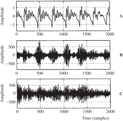
FIGURE 11.17 An example showing how TNS shapes quantization noise to conceal it under the transient envelope. A. The original speech signal. B. The quantization coding noise shaped with TNS. C. The quantization coding noise without TNS; masking is not utilized as well. (Herre and Johnston, 1997)

It should be emphasized that TNS prediction is done over frequency, and not over time. Thus the prediction error is shaped in time as opposed to frequency. Time resolution is increased as opposed to frequency resolution; temporal spread of quantization noise is reduced in the output decoded signal. TNS thus allows the encoder to control temporal pre-echo quantization noise within a filter-bank window by shaping it according to the audio signal, so that the noise is masked by the temporal audio signal, as shown in Fig. 11.17. TNS allows better coding of both transient content and pitch-based signals such as speech. The impulses which comprise speech are not always effectively coded with traditional transform block switching and may demand instantaneous increases in bit rate. TNS minimizes unmasked pre-echo in pitch-based signals and reduces the peak bit demand. With TNS, the codec can also use the more efficient long-block mode more often without introducing artifacts, and can also perform better at low sampling frequencies. TNS effectively and dynamically adapts the codec between high-time resolution for transient signals and high-frequency resolution for stationary signals and is more efficient than other designs using switched windows. As explained by Juergen Herre, the prediction filter can be determined from the range of spectral coefficients corresponding to the target frequency range (for example, 4 kHz to 20 kHz) and by using DPCM predictive coding methods such as calculating the autocorrelation function of the coefficients and using the Levinson–Durban recursion algorithm. A single TNS prediction filter can be applied to the entire spectrum or different TNS prediction filters can be uniquely applied to different parts of a spectrum, and TNS can be omitted for some frequency regions. Thus the temporal quantization noise control can be applied in a frequency-dependent manner.

AAC Techniques and Performance

The input audio signal can be applied to a four-band polyphase quadrature mirror filter (PQMF) bank to create four equal-width, critically sampled frequency bands. This is used for the scalable sampling rate (SSR) profile. An MDCT is used to produce 256 spectral coefficients from each of the four bands, for a total of 1024 coefficients. Positive or negative gain control can be applied independently to each of the four bands. With SSR, lower sampling rate signals (with lower bit rates) can be obtained at the decoder by ignoring the upper PQMF bands. For example, bandwidths of 18, 12, and 6 kHz can be obtained by ignoring one, two, or three bands. This allows scalability with low decoder complexity.

Two stereo coding techniques are used in AAC: intensity coding and M/S (middle/side) coding. Both methods can be combined and applied to selective parts of the signal’s spectrum. M/S coding is applied between channel pairs that are symmetrically placed to the left and right of the listener; this helps avoid spatial unmasking. M/S coding can be selectively switched in time (block by block) and frequency (scale factor bands). M/S coding can control the imaging of coding noise that is separate from the imaging of the masking signal. High-frequency time-domain imaging must be preserved in transient signals. Intensity stereo coding considers that perception of high-frequency sounds is based on their energy-time envelopes. Thus, some signals can be conveyed with one set of spectral values, shared among channels. Envelope information is maintained by reconstructing each channel level. Intensity coding can be implemented between channel pairs, and among coupling channel elements. In the latter, channel spectra are shared between channel pairs. Also, coupling channels permit downmixing in which additional audio elements such as a voice-over can be added to a recording. Both of these techniques can be used on both stereo and 5.1 multichannel content.

In one listening test, multichannel MPEG-2 AAC at 320 kbps outperformed MPEG-2 Layer II BC at 640 kbps. MPEG-2 Layer II at 640 kbps did not outperform MPEG-2 AAC at 256 kbps. For five full-bandwidth channels, MPEG-2 AAC claims “indistinguishable quality” for bit rates as low as 256 kbps to 320 kbps. Stereo MPEG-2 AAC at 128 kbps is said to provide significantly better sound quality than MPEG-2 Layer II at 192 kbps or MPEG-2 Layer III at 128 kbps. MPEG-2 AAC at 96 kbps is comparable to MPEG-2 Layer II at 192 kbps or MPEG-2 Layer III at 128 kbps. Spectral band replication (SBR) can be applied to AAC codecs. This is sometimes known as High-Efficiency AAC (HE AAC) or aacPlus. With SBR, a bit rate of 24 kbps per channel, or 32 kbps to 40 kbps for stereo signals, can yield good results. The MPEG-4 and MPEG-7 standards are discussed in Chap. 15.

ATRAC Codec

The proprietary ATRAC (Adaptive TRansform Acoustic Coding) algorithm was developed to provide data reduction for the SDDS cinematic sound system and was subsequently employed in other applications such as the MiniDisc format. ATRAC uses a modified discrete cosine transform and psychoacoustic masking to achieve a 5:1 compression ratio; for example, data on a MiniDisc is stored at 292 kbps. ATRAC transform coding is based on nonuniform frequency and time splitting concepts, and assigns bits according to rules fixed by a bit allocation algorithm. The algorithm both observes the fixed threshold of hearing curve, and dynamically analyzes the audio program to take advantage of psychoacoustic effects such as masking. The original codec version is sometimes known as ATRAC1. ATRAC was developed by Sony Corporation.

An ATRAC encoder accepts a digital audio input and parses it into blocks. The audio signal is divided into three subbands, which are then transformed into the frequency domain using a variable block length. Transform coefficients are grouped into 52 subbands (called block floating units or BFUs) modeled on the ear’s critical bands, with particular resolution given to lower frequencies. Data in these bands is quantized according to dynamic sensitivity and masking characteristics based on a psychoacoustic model. During decoding, the quantized spectra are reconstructed according to the bit allocation method, and synthesized into the output audio signal.

ATRAC differs from some other codecs in that psychoacoustic principles are applied to both the bit allocation and the time-frequency splitting. In that respect, both subband and transform coding techniques are used. In addition, the transform block length adapts to the audio signal’s characteristics so that amplitude and time resolution can be varied between static and transient musical passages. Through this processing, the data rate is reduced by 4/5. The ATRAC encoding algorithm can be considered in three parts: time-frequency analysis, bit allocation, and quantization of spectral components. The analysis portion of the algorithm decomposes the signal into spectral coefficients grouped into BFUs that emulate critical bands. The bit allocation portion of the algorithm divides available bits between the BFUs, allocating more bits to perceptually sensitive units. The quantization portion of the algorithm quantizes each spectral coefficient to the specified word length.

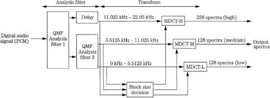
FIGURE 11.18 The ATRAC encoder time-frequency analysis block contains QMF filter banks and MDCT transforms to analyze the signal.

The time-frequency analysis, shown in Fig. 11.18, uses subband and transform coding techniques. Two quadrature mirror filters (QMFs) divide the input signal into three subbands: low (0 Hz to 5.5125 kHz), medium (5.5125 kHz to 11.025 kHz), and high (11.025 kHz to 22.05 kHz). The QMF banks ensure that time-domain aliasing caused by the subband decomposition will be canceled during reconstruction. Following splitting, contents are examined to determine the length of block durations. Signals in each of these bands are then placed in the frequency domain with the MDCT algorithm. The MDCT allows up to a 50% overlap between adjacent time-domain windows; this maintains frequency resolution at critical sampling. A total of 512 coefficients are output, with 128 spectra in the low band, 128 spectra in the mid band, and 256 spectra in the high band.

Transform coders must balance frequency resolution with temporal resolution. A long block size achieves high frequency resolution and quantization noise is readily masked by simultaneous masking; this is appropriate for a steady-state signal. However, transient signals require temporal resolution, otherwise quantization noise will be spread in time over the block of samples; a pre-echo can be audible prior to the onset of the transient masker. Thus, instead of a fixed transform block length, the ATRAC algorithm adaptively performs nonuniform time splitting with blocks that vary according to the audio program content. Two modes are used: long mode (11.6 ms in the high-, medium-, and low-frequency bands) and short mode (1.45 ms in the high-frequency band, and 2.9 ms in the mid- and low-frequency bands). The long block mode yields a narrow frequency band, and the short block mode yields wider frequency bands, trading time and frequency resolution as required by the audio signal. Specifically, transient attacks prompt a decrease in block duration (to 1.45 ms or 2.9 ms), and a more slowly changing program promotes an increase in block duration (to 11.6 ms). Block duration is interactive with frequency bandwidth; longer block durations permit selection of narrower frequency bands and greater resolution. This time splitting is based on the effect of temporal pre-masking (backward masking) in which tones sounding close in time exhibit masking properties.

Normally, the long mode provides good frequency resolution. However, with transients, quantization noise is spread over the entire signal block and the initial quantization noise is not masked. Thus, when a transient is detected, the algorithm switches to the short mode. Because the noise is limited to a short duration before the onset of the transient, it is masked by pre-masking. Because of its greater extent, post-masking (forward masking) can be relied on to mask any signal decay in the long mode. The block size mode can be selected independently for each band. For example, a long block mode might be selected in the low-frequency band, and short modes in the mid- and high-frequency bands.

The MDCT frequency domain coefficients are then grouped into 52 BFUs; each contains a fixed number of coefficients. As noted, in the long mode, each unit conveys 11.6 ms of a narrow frequency band, and in the short mode each block conveys 1.45 ms or 2.9 ms of a wider frequency band. Fifty-two nonuniform BFUs are present across the frequency range; there are more BFUs at low frequencies, and fewer at high frequencies. This nonlinear division is based on the concept of critical bands. In the ATRAC model, for example, the band centered at 150 Hz is 100 Hz wide, the band at 1 kHz is 160 Hz wide, and the band at 10.5 kHz is 2500 Hz wide. These widths reflect the ear’s decreasing sensitivity to high frequencies.

Each of the 512 spectral coefficients is quantized according to scale factor and word length. The scale factor defines the full-scale range of the quantization. It is selected from a list of possibilities and describes the magnitude of the spectral coefficients in each of the 52 BFUs. The word length defines the precision within each scale; it is calculated by the bit allocation algorithm as described below. All the coefficients in a given BFU are given the same scale factor and quantization word length because of the psychoacoustic similarity within each group. Thus the following information is coded for each frame of 512 values: MDCT block size mode (long or short), word length for each BFU, scale factor for each BFU, and quantized spectral coefficients.

The bit allocation algorithm considers the minimum threshold curve and simultaneous masking conditions applicable to the BFUs, operating to yield a reduced data rate. Available bits must be divided optimally between the block floating units. BFUs coded with many bits will have low quantization noise, but BFUs with few bits will have greater noise. ATRAC does not specify an arbitrary bit allocation algorithm; this allows improvement in future encoder versions. The decoder is completely independent of any allocation algorithm, also allowing future improvement. To some extent, because the time-frequency splitting relies on critical band and pre-masking considerations, the choice of the bit allocation algorithm is less critical. However, any algorithm must minimize perceptual error.

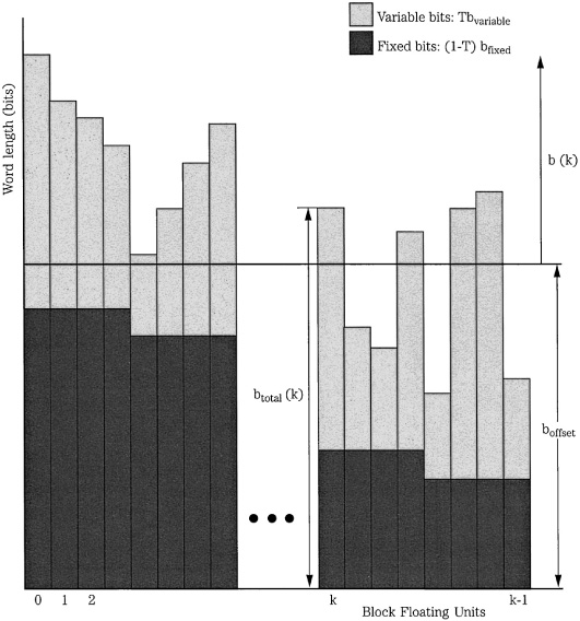
FIGURE 11.19 An example of a bit-allocation algorithm showing the bit assignment, using both fixed and variable bits. Fixed bits are weighted toward low-frequency BFU regions. Variable bits are assigned according to the logarithm of the spectral coefficients in each BFU. (Tsutsui et al., 1996)

One example of a bit allocation model declares both fixed and variable bits, as shown in Fig. 11.19. Fixed bits are allocated mainly to low-frequency BFU regions, emphasizing their perceptual importance. Variable bits are assigned according to the logarithm of the spectral coefficients in each BFU. The total bit allocation b_total for each BFU is the weighted sum of the fixed bits b_fixed(k) and the variable bits b_variable(k) in each BFU. Thus, for each BFU k:

The weight T describes the tonality of the signal, taking a value close to 0 for nontonal signals, and a value close to 1 for tonal signals. Thus the proportion of fixed bits to variable bits is itself variable. For example, for noise-like signals the allocation emphasizes fixed bits, thus decreasing the number of bits devoted to insensitive high frequencies. For pure tones, the allocation emphasizes variable bits, concentrating available bits to a few sensitive BFUs with tonal components.

However, the allocation method must observe the overall bit rate. The previous equation does not account for this and will generally allocate more bits than available. To maintain a fixed and limited bit rate, an offset b_offset is devised, and set equal for all BFUs. The offset is subtracted from b_total(k) for each BFU, yielding the final bit allocation b_final(k):

If the final value describes a negative word length, that BFU is given zero bits. Because low frequencies are given a greater number of fixed bits, they generally need fewer variable bits to achieve the offset threshold, and become coded (see Fig. 11.19). To meet the required output bit rate, the global bit allocation can be raised or lowered by correspondingly raising or lowering the threshold of masking. As noted, ATRAC does not specify this, or any other arbitrary allocation algorithm.

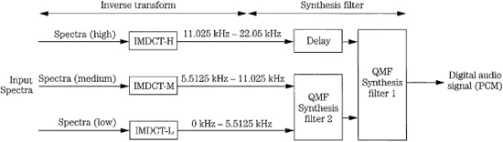
FIGURE 11.20 The ATRAC decoder time-frequency synthesis block contains QMF banks and MDCT transforms to synthesize and reconstruct the signal.

The ATRAC decoder essentially reverses the encoding process, performing spectral reconstruction and time-frequency synthesis. Time-frequency synthesis is shown in Fig. 11.20. The decoder first accepts the quantized spectral coefficients, and uses the word length and scale factor parameters to reconstruct the MDCT spectral coefficients. To reconstruct the audio signal, these coefficients are first transformed back into the time domain by the inverse MDCT (IMDCT), using either long or short mode blocks as specified by the received parameters. The three time-domain subband signals are synthesized into the output signal using QMF synthesis banks, obtaining a full spectrum, 16-bit digital audio signal. Wideband quantization noise introduced during encoding (to achieve data reduction) is limited to critical bands, where it is masked by signal energy in each band.

Other versions of ATRAC were developed. ATRAC3 achieves twice the compression of ATRAC1 while providing similar sound quality operating at bit rates such as 128 kbps. The broadband audio signal is split into four subbands using a QMF bank; the bands are 0 Hz to 2.75625 kHz, 2.75625 kHz to 5.5125 kHz, 5.5125 kHz to 11.025 kHz, and 11.025 kHz to 22.05 kHz. Gain control is applied to each band to minimize pre-echo. When a transient occurs, the amplitude of the section preceding the attack is increased. Gain is correspondingly decreased during decoding, effectively attenuating pre-echo. The subbands are applied to fixed-length MDCT with 256 components. Tonal components are subtracted from the signal and analyzed and quantized separately. Entropy coding is applied. In addition, joint stereo coding can be used adaptively for each band.

The ATRAC3plus codec is designed to operate at generally lower bit rates; rates of 48, 64, 132, and 256 kbps are often used. The broadband audio signal is processed in 16 subbands; a window of up to 4096 samples (92 ms) can be used and bits can be allocated unequally over two channels.

The ATRAC Advanced Lossless (AAL) codec provides scalable lossless compression. It codes ATRAC3 or ATRAC3plus data as well as residual information that is otherwise lost. The ATRAC3 or ATRAC3plus data can be decoded alone for lossy reproduction or the residual can be added for lossless reproduction.

Perceptual Audio Coding (PAC) Codec

The Perceptual Audio Coding (PAC) codec was designed to provide audio coding with bit rates ranging from 6 kbps for a monophonic channel to 1024 kbps for a 5.1-channel format. It was particularly aimed at digital audio broadcast and Internet download applications, at a rate of 128 kbps for two-channel near-CD quality coding; however, 96 kbps may be used for FM quality. PAC employs coding methods that remove signal perceptual irrelevancy, as well as source coding to remove signal redundancy, to achieve a reduction ratio of about 11:1 while maintaining transparency. PAC is a third-generation codec with PXFM and ASPEC as its antecedents, the latter also providing the ancestral basis for MPEG-1 Layer III. PAC was developed by AT&T and Bell Laboratories of Lucent Technologies.

The architecture of a PAC encoder is similar to that of other perceptual codecs. Throughout the algorithm, data is placed in blocks of 1024 samples per channel. An MDCT filter bank converts time-domain audio signals to the frequency domain; a hybrid filter is not used. The MDCT uses an adaptive window size to control quantization noise spreading, where the spreading is greater in the time domain with a longer 2048-point window and greater in the frequency domain with a series of shorter 256-point windows. Specifically, a frequency resolution of 1024 uniformly spaced frequency bands (a window of 2048 points) is usually employed. When signal transient characteristics suggest that pre-echo artifacts may occur, the filter bank adaptively switches to a transform with 128 bands. In either case, the perceptual model calculates a frequency-domain masking threshold to determine the maximum quantization noise that can be added to each frequency band without an audible penalty. The perceptual model used in PAC to code monophonic signals is similar to the MPEG-1 psychoacoustic model 2.

The audio signal, represented as spectral coefficients, is requantized to one of 128 exponentially distributed quantization step sizes according to noise allocation determinations. The codec uses a variety of frequency band groupings. A fixed “threshold calculation partition” is a set of one-to-many adjacent filter bank outputs arranged to create a partition width that is about 1/3 of a critical band. Fixed “coder bands” consist of a multiple of four adjacent filter bank outputs, ranging from 4 to 32 outputs, yielding a bandwidth as close to 1/3 critical band as possible. There are 49 coder bands for the 1024-point mode and 14 coder bands for the 128-point filter mode. An iterative rate control loop is used to determine quantization relative to masking thresholds. Time buffering may be used to smooth the resulting bit rate. Coder bands are assigned one scale factor. “Sections” are data dependent groupings of adjacent coder bands using the same Huffman codeword. Coefficients in each coder band are encoded using one of 16 Huffman codebooks.

At the codec output, a formatter generates a packetized bitstream. One 1024-sample block (or eight 128-sample blocks) from each channel are placed in one packet, regardless of the number of channels. The size of a packet corresponding to each 1024 input samples is thus variable. Depending on the reliability of the transmission medium, additional header information is added to the first frame, or to every frame. A header may contain data such as synchronization, error correction, sample rate, number of channels, and transmission bit rate.

For joint-stereo coding, the codec employs a binary masking level difference (BMLD) using M (monaural, L+R), S (stereo, L-R) and independent L and R thresholds. M-S versus L-R coding decisions are made independently for each band. The multi-channel MPAC codec (for example, coding 5.1 channels) computes individual masking thresholds for each channel, two pairs (front and surround) of M-S thresholds, as well as a global threshold based on all channels. The global threshold takes advantages of masking across all channels and is used when the bit pool is close to depletion.

PAC employs unequal error protection (UEP) to more carefully protect some portions of the data. For example, corrupted control information could lead to a catastrophic loss of synchronization. Moreover, some errors in audio data are more disruptive than others. For example, distortion in midrange frequencies is more apparent than a loss of stereo separation. Different versions of PAC are available for DAB and Internet applications; they are optimized for different transmission error conditions and error concealment. The error concealment algorithm mitigates the effect of bit errors and corrupted or lost packets; partial information is used along with heuristic interpolation. There is slight audible degradation with 5% random packet losses and the algorithm is effective with 10 to 15% packet losses.

As with most codecs, PAC has evolved. PAC version 1.A is optimized for unim-paired channel transmission of voice and music with up to 8-kHz bandwidth; bit rates range from 16 kbps to 32 kbps. PAC version 1.B uses a bandwidth of 6.5 kHz. PAC version 2 is designed for impaired channel broadcast applications, with bit rates of 16 kbps to 128 kbps for stereo signals. PAC version 3 is optimized for 64 kbps with a bandwidth of about 13 kHz. PAC version 4 is optimized for 5.1-channel sound. EPAC is an enhanced version of PAC optimized for low bit rates. Its filter switches between two different filter-bank designs depending on signal conditions. At 128 kbps, EPAC offers CD-trans-parent stereo sound and is compliant with RealNetwork’s G2 streaming Internet player. In some applications, monaural MPAC codecs are used to code multichannel audio using a perceptual model with provisions for spatial coding conditions such as binaural unmasking effects and binary-level masking differences. Signal pairs are coded and masking thresholds are computed for each channel.

AC-3 (Dolby Digital) Codec

Many data reduction codecs are designed for a variety of applications. The AC-3 (Dolby Digital) codec in particular is widely used to convey multichannel audio in applications such as DTV, DBS, DVD-Video, and Blu-ray. The AC-3 codec was preceded by the AC-1 and AC-2 codecs.

The AC-1 (Audio Coding-1) stereo codec uses adaptive delta modulation, as described in Chap. 4, combined with analog companding; it is not a perceptual codec. An AC-1 codec can code a 20-kHz bandwidth stereo audio signal into a 512-kbps bitstream (approximately a 3:1 reduction). AC-1 was used in satellite relays of television and FM programming, as well as cable radio services.

The AC-2 codec is a family of four single-channel codecs used in two-channel or multichannel applications. It was designed for point-to-point transmission such as full-duplex ISBN applications. AC-2 is a perceptual codec using a low-complexity time-domain aliasing cancellation (TDAC) transform. It divides a wideband signal into multiple subbands using a 512-sample 50% overlapping FFT algorithm performing alternating modified discrete cosine and sine transform (MDCT/MDST) calculations; a 128-sample FFT can be used for low-delay coding. A window function based on the Kaiser–Bessel kernel is used in the window design. Coefficients are grouped into subbands containing from 1 to 15 coefficients to model critical bandwidths. The bit allocation process is backward-adaptive in which bit assignments are computed equivalently at both the encoder and decoder. The decoder uses a perceptual model to extract bit allocation information from the spectral envelope of the transmitted signal. This effectively reduces the bit rate, at the expense of decoder complexity. Subbands have preallocated bits, with the lower subbands receiving a greater share. Additional bits are adaptively drawn from a pool and assigned according to the logarithm of peak energy levels in subbands. Coefficients are quantized according to bit allocation calculations, and blocks are formed. Algorithm parameters vary according to sampling frequency. At sampling frequencies of 48, 44.1, and 32 kHz, the following apply: bytes/block: 168, 184, 190; total bits: 1344, 1472, 1520; subbands: 40, 43, 42; adaptive bits: 225, 239, 183.

The AC-2 codec provides high audio quality with a data rate of 256 kbps per channel. With 16-bit input, reduction ratios include 6.1:1, 5.6:1, and 5.4:1 for sample rates of 48, 44.1, and 32 kHz, respectively. AC-2 is also used at 128 kbps and 192 kbps per channel. AC-2 is a registered .wav type so that AC-2 files are interchangeable between computer platforms. The AC-2 .wav header contains an auxiliary data field at the end of each block, selectable from 0 to 32 bits. For example, peak levels can be stored to facilitate viewing and editing of .wav files. AC-2 codec applications include PC sound cards, studio/transmitter links, and ISDN linking of recording studios for long distance recording. The AC-2 bitstream is robust against errors. Depending on the implementation, AC-2 delay varies between 7 ms and 60 ms. AC-2A is a multirate, adaptive block codec, designed for higher reduction ratios; it uses a 512/128-point TDAC filter. AC-2 was introduced in 1989.

AC-3 Overview

The AC-3 coding system (popularly known as Dolby Digital) is an outgrowth of the AC-2 encoding format, as well as applications in commercial cinema. AC-3 was first introduced in 1992. AC-3 is a perceptual codec designed to process an ensemble of audio channels. It can code from 1 to 7 channels as 3/3, 3/2, 3/1, 3/0, 2/2, 2/1, 2/0, 1/0, as well as an optional low-frequency effects (LFE) channel. AC-3 is often used to provide a 5.1 multichannel surround format with left, center right, left-surround, right-surround, and an LFE channel. The frequency response of the main channels is 3 Hz to 20 kHz, and the frequency response of the LFE channel is 3 Hz to 120 Hz. These six channels (requiring 6 × 48 kHz × 18 bits = 5.184 Mbps in uncompressed PCM representation) can be coded at a nominal rate of 384 kbps, with a bandwidth reduction of about 13:1. However, the AC-3 standard also supports bit rates ranging from 32 kbps to 640 kbps. The AC-3 codec is backward compatible with matrix surround sound formats, two-channel stereo, and monaural reproduction; all of these can be decoded from the AC-3 data stream. AC-3 does not use 5.1 matrixing in its bitstream. This ensures that quantization noise is not directed to an incorrect channel, where it could be unmasked. AC-3 transmits a discrete multichannel coded bitstream, with digital downmixing in the decoder to create the appropriate number (monaural, stereo, matrix surround, or full multichannel) of reproduction channels.

AC-3 contains a dialogue normalization level control so that the reproduced level of dialogue (or any audio content) is uniform for different programs and channels. With dialogue normalization, a listener can select a playback volume and the decoder will automatically replay content at that average relative level regardless of how it was recorded. AC-3 also contains a dynamic range control feature. Control data can be placed in the bitstream so that a program’s recorded dynamic range can be varied in the decoder over a ±24-dB range. Thus, the decoder can alter the dynamic range of a program to suit the listener’s preference (for example, a reduced dynamic range “midnight mode”). AC-3 also provides a downmixing feature; a multichannel recording can be reduced to stereo or monaural. The mixing engineer can specify relative interchannel levels. Additional services can be embedded in the bitstream including verbal description for the visually impaired, dialogue with enhanced intelligibility for the hearing impaired, commentary, and a second stereo program. All services may be tagged to indicate language. AC-3 facilitates editing on a block level, and blocks can be rocked back and forth at the decoder, and read as forward and reverse audio. Complete encoding/decoding delay is typically 100 ms.

Because AC-3 eliminates redundancies between channels, greater coding efficiency is achieved relative to AC-2; a stereo version of AC-3 provides high quality with a data rate of 192 kbps. In one test, AC-3 at 192 kbps scored 4.5 on the ITU-R impairment scale. Differences between the original and coded files were perceptible to expert listeners, but not annoying. The AC-3 format also delivers data describing a program’s original production format (monaural, stereo, matrix, and the like), can encode parameters for selectable dynamic range compression, can route low bass only to those speakers with subwoofers, and provide gain control of a program.

AC-3 uses hybrid backward/forward adaptive bit allocation in which an adaptive allocation routine operates in both the encoder and decoder. The model defines the spectral envelope, which is encoded in the bitstream. The encoder contains a core psychoacoustic model, but can employ a different model and compare results. If desired, the encoder can use the data syntax to code parameter variations in the core model, or convey explicit delta bit allocation information, to improve results. Block diagrams of an AC-3 encoder and decoder are shown in Fig. 11.21.

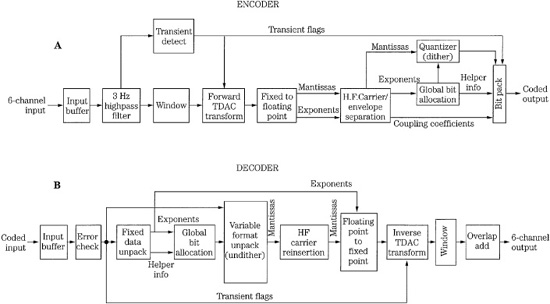
FIGURE 11.21 The AC-3 (Dolby Digital) adaptive transform encoder and decoder. This codec can provide 5.1-channel surround sound. A. AC-3 encoder. B. AC-3 decoder.

AC-3 achieves its data reduction by quantizing a frequency-domain representation of the audio signal. The encoder first uses an analysis filter bank to transform time-domain PCM samples into frequency-domain coefficients. Each coefficient is represented in binary exponential notation as a binary exponent and mantissa. Sets of exponents are encoded into a coarse representation of the signal spectrum and referred to as the spectral envelope. This spectral envelope is used by the bit allocation routine to determine the number of bits needed to code each mantissa. The spectral envelope and quantized mantissas for six audio blocks (1536 audio samples) are formatted into a frame for transmission.

The decoding process is the inverse of the encoding process. The decoder synchronizes the received bitstream, checks for errors, and de-formats the data to recover the encoded spectral envelope and quantized mantissas. The bit allocation routine and the results are used to unpack and de-quantize the mantissas. The spectral envelope is decoded to yield the exponents. Finally, the exponents and mantissas are transformed back to the time domain to produce output PCM samples.

AC-3 Theory of Operation

Operation of the AC-3 encoder is complex, with much dynamic optimization performed. In the encoder, blocks of 512 samples are collected and highpass filtered at 3 Hz to eliminate dc offset and analyzed with a bandpass filter to detect transients. Blocks are windowed and processed with a signal-adaptive transform codec using a critically sampled filter bank with time-domain aliasing cancellation (TDAC) described by Princen and Bradley. An FFT is employed to implement an MDCT algorithm. Frequency resolution is 93.75 Hz at 48 kHz; each transform block represents 10.66 ms of audio, but transforms are computed every 5.33 ms so the audio block rate is 187.5 Hz. Because there is a 50% long-window overlap (an optimal window function based on the Kaiser–Bessel kernel is used in the window design), each PCM sample is represented in two sequential transform blocks; coefficients are decimated by a factor of two to yield 256 coefficients per block. Aliasing from sub-sampling is exactly canceled during reconstruction. The transformation allows the redundancy introduced in the blocking process to be removed. The input to the TDAC is 512 time-domain samples while the output is 256 frequency-domain coefficients. There are 50 bands between 0 Hz and 24 kHz; the bandwidths vary between 3.4 and 1.4 of critical bandwidth values.

Time-domain transients such as an impulsive sound might create audible quantization artifacts. A transient detector in the encoder, using a high-frequency bandpass filter, can trigger window switching to dynamically halve the transform length from 512 to 256 samples for a finer time resolution. The 512-sample transform is replaced by two 256-sample transforms, each producing 128 unique coefficients; time resolution is doubled, to help ensure that quantization noise is concealed by temporal masking. Audio blocks are 5.33 ms, and transforms are computed every 2.67 ms at 48 kHz. Short blocks use an asymmetric window that uses only one-half of a long window. This yields poor frequency selectivity and does not give a smooth crossfade between blocks. However, because short blocks are only used for transient signals, the signal’s flat and wide spectrum does not require selectivity and the transient itself will mask artifacts. This block switching also simplifies processing, because groups of short blocks can be treated as groups of long blocks and no special handling is needed.

Coefficients are grouped into subbands that emulate critical bands. Each frequency coefficient is processed with floating-point representation with mantissa (0 to 16 bits) and exponent (5 bit) to maintain dynamic range. Coefficient precision is typically 16 to 18 bits but may reach 24 bits. The coded exponents act as scale factors for mantissas and represent the signal’s spectrum; their representation is referred to as the spectral envelope. This spectral envelope coding permits variable resolution of time and frequency. Unlike some codecs, to reduce the number of exponents conveyed, AC-3 does not choose one exponent, based on the coefficient with the largest magnitude, to represent each band. In AC-3, fine-grained exponents are used to represent each coefficient, and efficiency is achieved by differential coding and sharing of exponents across frequency and time. The spectral envelope is coded as the difference between adjacent filters; because the filter response falls off at 12 dB/bin, maximum deltas of 2 (1 represents a 6-dB difference) are needed. The first dc term is coded as an absolute, and other exponents are coded as one of five changes (±2, ±1, 0) from the previous lower frequency exponent, allowing for ±12 dB/bin differences in exponents.

AC-3 Exponent Strategies and Bit Allocation

For improved bit efficiency, the differential exponents are combined into groups in the audio block. One, two, or four mantissas can use the same exponent. These groupings are known as D15, D25, or D45 modes, respectively, and are referred to as exponent strategies. The number of grouped differential exponents placed in the audio block for a channel depends on the exponent strategy and the frequency bandwidth of that channel. The number of exponents in each group depends only on the exponent strategy, which is based on the need to minimize audibility of quantization noise. In D15 exponent coding of the spectral envelope (2.33 bits per exponent), groups of three differentials are coded in a 7-bit word; D15 provides fine frequency resolution at the expense of temporal resolution. It is used when the audio signal envelope is relatively constant over many audio blocks. Because D15 is conveyed when the spectrum is stable, the estimate is coded only occasionally, for example, once every six blocks (32 ms) yielding 0.39 bits per audio sample.

The spectral estimate must be updated more frequently when transient signals are coded. The spectral envelope must follow the time variations in the signal; this estimate is coded with less frequency resolution. Two methods are used. D25 provides moderate frequency resolution and moderate temporal resolution. Coefficients are shared across frequency pairs. A delta is coded for every other frequency coefficient; the data rate is 1.17 bits per exponent. D25 is used when the spectrum is stable over two to three blocks, and then significantly changes. In the D45 coding, one delta is coded for every four coefficients; the data rate is 0.58 bits per exponent. D45 provides high temporal resolution and low frequency resolution. It is used when transients occur within single audio blocks. The encoder selects the exponent coding method (D15, D25, D45, or REUSE) for every audio block and places this in a 2-bit exponent strategy field. Because the exponent selection is coded in the bitstream, the decoder tracks the results of any encoder methodology. Examples of the D15, D25, and D45 modes are shown in Fig. 11.22.

Exponents can also be shared across time. Signals may be stationary for longer than a 512-sample block and have similar spectral content over many blocks. Thus, exponents can be reused for subsequent blocks. In most cases, D15 is coded in the first block in a frame, and reused for the next five blocks. This can reduce the exponent data rate by a factor of 6, to 0.10 bits per exponent.

Most encoders use a forward-adaptive psychoacoustics model and bit allocation that analyzes the signal spectrum and quantizes mantissa values and sends them to the decoder; all modeling and allocation is done in the encoder. In contrast, the AC-3 encoder contains a forward-backward adaptive psychoacoustics model that determines the masked threshold and quantization, and the decoder also contains the core backward-adaptive model. This reduces the amount of bit allocation information that must be conveyed. The encoder bases bit allocation on exponent values, and because the decoder receives the exponent values, it can backward-adaptively recompute the corresponding bit allocation. The approach allows overall lower bit rates, at the expense of increased decoder complexity. Also, this limits the ability to revise the psychoacoustic model in the encoder while retaining compatibility with existing decoders. This is addressed with a parametric model, and by providing for a forward-adaptive delta correction factor.

In the encoder, the forward-adaptive model uses an iterative rate control loop to determine the model’s parameters defining offsets of maskers from a masking contour. These are used by the backward-adaptive model, along with quantized spectral envelope information, to estimate the masked threshold. The perceptual model’s parameters and an optional forward-adaptive delta bit allocation that can adjust the masking thresholds are conveyed to the decoder.

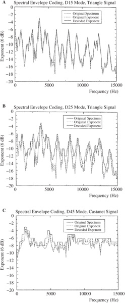
FIGURE 11.22 Three examples of spectral envelope (exponent) coding strategies used in the AC-3 codec. A. D15 mode coding for a triangle signal. B. D25 mode coding for a triangle signal. C. D45 mode coding for a castanet signal. (Todd et al., 1994)

The encoder’s bit allocation delta parameter can be used to upgrade the encoder’s functionality. Future encoders could employ two perceptual models, the original version and an improved version, and the encoder could convey a masking level adjustment.

The bit allocation routine analyzes the spectral envelope of the audio signal according to masking criteria to determine the number of bits to assign to each mantissa. Ideally, allocation is calculated so that the SNR for quantized mantissas is greater than or equal to the SMR. There are no preassigned mantissa or exponent bits; assignment is performed globally on all channels from a bit pool. The routine interacts with the parametric perceptual model to estimate audible and inaudible spectral components. The estimated noise level threshold is computed for 50 bands of nonuniform bandwidth (approximately 1.6 octaves). The bit allocation for each mantissa is determined by a lookup table based on the difference between the input signal power spectral density (psd) along a fine-grain uniform frequency scale, and estimated noise level threshold along a banded coarse-grain frequency scale. The routine considers the decoded spectral envelope to be the power spectral density of the signal. This signal is effectively convolved, using two IIR filters for the two-slope spreading function, with a simplified spreading function that represents the ear’s masking response. The spreading function is approximated by two masking curves: a fast-decaying upward curve and slow-decaying upward curve, which is offset downward in level. The curves are referred to as a fast leak and slow leak. Convolution is performed starting at the lowest frequency psd. Each new psd is compared to current leak values and judged to be significant or not; this yields the predicted masking value for each band. The shape of the spreading function is conveyed to the decoder by four parameters.

This predicted curve is compared to a hearing threshold, and the larger of the values is used at each frequency point to yield a global masking curve. The resulting predicted masking curve is subtracted from the original unbanded psd to determine the SNR value for each transform coefficient. These are used to quantize each coefficient mantissa from 0 to 16 bits. Odd-symmetric quantization (the mantissa range is divided by an odd number of steps that are equal in width and symmetric about zero) is used for all low-precision quantizer levels (3-, 5-, 7-, 11-, 15-level) to avoid biases in coding, and even-symmetric quantization (the first step is 50% shorter and the last step is 50% longer than the rest) is used for all other quantization levels (from 32-level through 65,536-level).

Bits are taken iteratively from a common bit pool available to all channels. Mantissa quantization is adjusted to use the available bit rate. The effect of interchannel masking is relatively slight. To minimize audible quantization noise at low frequencies where frequency resolution is relatively low, the noise from coefficients is examined and bits are iteratively added to lower noise where necessary. Quantized mantissas are scaled and offset. Subtractive dither is optionally employed when zero bits are allocated to the mantissa. A pseudo-random number generator can be used. A mode bit indicates when dither is used and provides synchronization to the decoder’s subtractive dither circuit. In addition, the carrier portion of high-frequency localization information is removed, and the envelope is coded instead; high-frequency multichannel carrier content may be combined into a coupling channel.

AC-3 Multichannel Coding

One of the hallmarks of AC-3 coding is its ability to efficiently code an ensemble of multiple channels to a single low bit-rate bitstream. To achieve greater bit efficiency, the encoder may use channel coupling and rematrixing on selective frequencies while preserving perceptual spatial accuracy. Channel coupling, based on intensity stereo coding, combines the high-frequency content of two or more channels into one coupling channel. The combined coupling channel, along with coupling coordinates, the quantized power spectral ratios between each channel’s original signal and the coupled channel, are conveyed for decoding and reconstructing the original energy envelopes. Coupling may be performed at low bit rates, when signal conditions exceed the bit rate. It efficiently (but perhaps not transparently) codes a multichannel signal, taking into account high-frequency directionality limitations in human hearing, without reducing audio bandwidth. Above 3 kHz, the ear is unable to distinguish the fine temporal structure of high-frequency waveforms and instead relies on the envelope energy of the sounds. In other words, at high frequencies, we are not sensitive to phase, but only to amplitude. Directionality is determined by the interaural time delay of the envelope and by perceived frequency response based on head shadowing. As a result, the ear cannot independently detect the direction of two high-frequency sounds that are close in frequency.

Coupling can yield significant bit-rate reduction. As Steve Vernon points out, given the critical band resolution, high-frequency mantissa magnitudes do not need to be accurately coded for individual frequency bins, as long as the overall signal energy in each critical band is correct. Because 85% of transform coefficients are above 3 kHz, large amounts of error are acceptable in high-frequency bands.

The AC-3 codec can couple channels at high frequencies; care is taken to avoid phase cancellation of the common channels. The coupling strategy is determined wholly in the encoder. Coupling coordinates for each individual channel are used to code the ratio of original signal power in a band to the coupling channel power in each band. Coupling channels are encoded in the same way as individual channels with a spectral envelope comprising exponents and mantissas. Frequencies below a certain coupling frequency (a range of 3 kHz to 20 kHz is possible, with 10 kHz being typical) are encoded as individual channels, and encoded as coupling coordinates above the coupling frequency. With a 10-kHz coupling frequency, the data rate for exponents and mantissas is nearly halved. Half of the exponents and mantissas for each coupled channel are discarded. Only the exponents and mantissas for the coupling channel, and scale factors, are conveyed.

Figure 11.23A shows an example of channel coupling of three channels. Phase is adjusted to prevent cancellation when summing channels. The monaural coupled channel is created by summing the input coupled-channel spectral coefficients above the coupling frequency. The signal energy in each critical band of the input channels and coupled channel are computed and used to determine coupling coordinate scale factors. The energy in each band of each coupled channel is divided by the energy in each corresponding band of the coupling channel. The scale factors thus represent the amount that the decoder will scale the coupling-channel bands to re-create bands of the original energy. The dynamic range of the scaling factors may range from −132 to +18 dB with a resolution between 0.28 dB to 0.53 dB. One to 18 frequency bands may be used, with 14 bands being typical. During decoding, individual channel-coupling coordinates are multiplied by the coupling-channel coefficients to regenerate individual high-frequency coefficients. Figure 11.23B shows how three coupled channels are decoded.

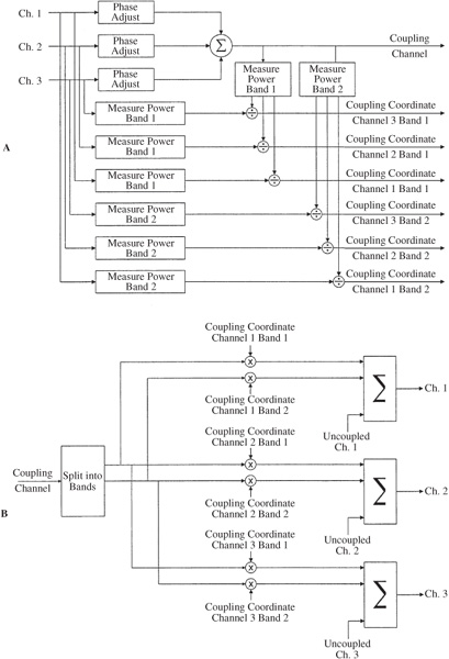
FIGURE 11.23 The AC-3 codec can couple audio channels at high frequencies. In this illustration, three channels are coupled to form one coupling channel. A. Encode coupling process. B. Decode coupling process. (Fielder, 1996)

The encoder may also use rematrixing coding, similar to M/S coding, to exploit the correlation between channel pairs. Rather than code the spectra of right and left (R, L) channels independently, the sum and difference (R, L) is coded. For example, when the R and L channels are identical, no bits are allocated to the R channel. Rematrixing is applied selectively to up to four frequency regions; the regions are based on coupling information. Rematrixing is not used in coupling channels but can be used simultaneously with coupling. If used with coupling, the rematrixing frequency region ends at the start of the coupling region. Rematrixing coding is only used in 2/0 channel mode, and is compatible with Dolby Pro Logic and other matrix systems.

If matrixing is not used and a decoded perceptually coded monaural signal is played through a matrix decoder, small differences in quantization noise between the two channels could cause the matrix system to derive a surround channel from the noise differences between channels, and thus direct unmasked quantization noise to the surround channels. Moreover, the noise will be modulated by the center-channel signal, further increasing audibility. Rematrixing ensures that when the input signals are highly correlated, the quantization noise is also highly correlated. Thus, when a rematrixed two-channel AC-3 signal is played through a matrix system, quantization noise will not be unmasked.

AC-3 Bitstream and Decoder

Data in an AC-3 bitstream is contained in frames, as shown in Fig. 11.24. Each frame is an independently encoded entity. A frame contains a synchronization information (SI) header, bitstream information (BSI) header, 32 milliseconds of audio data as quantized frequency coefficients, auxiliary field, and CRCC error detection data. The frame period is 32 milliseconds at a 48-kHz sampling frequency. The SI field contains a 16-bit synchronization word, 2-bit sampling rate code, and 6-bit frame size code. The BSI field describes the audio data with information such as coding mode, timecode, copyright, normalized dialogue level, and language code. Audio blocks are variable length, but six transform blocks, with 256 samples per block (1536 in total), must fit in one frame. Audio blocks mainly comprise quantized mantissas, exponent strategy, differentially coded exponents, coupling data, rematrixing data, block switch flags, dither flags, and bit allocation parameters. Each block contains data for all coded channels. A frame holds a constant number of bits based on the bit rate. However, audio block boundaries are not fixed. This allows the encoder to globally allocate bitstream resources where needed.

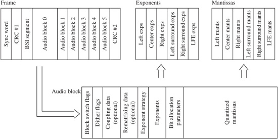
FIGURE 11.24 Structure of the AC-3 bitstream showing blocks in an audio frame. (Vernon, 1999)

One 16-bit CRCC word is contained at the end of each frame, and an additional 16-bit CRCC word may be optionally placed in the SI header. In each case, the generating polynomial is x¹⁶ +x¹⁵ + x² + 1. Error detection and the response to errors vary in different AC-3 applications. Error concealment can be used in which a previous audio segment is repeated to cover a burst error. The decoder does not decode erroneous data; this could lead to invalid bit allocation. The first block always contains a complete refresh of all decoding information. Unused block areas may be used for auxiliary data. Audio data is placed in the bitstream so that the decoder can begin to output a signal before starting to decode the second block. This reduces the memory requirements in the decoder because it does not need to store parameters for more than one block at a time.

One or more AC-3 streams may be conveyed in an MPEG-2 transport stream as defined in the ISO/IEC 13818-1 standard. The stream is packetized as PES packets. It is not necessary to unambiguously indicate that a stream is AC-3. The MPEG-2 standard does not contain codes to indicate an AC-3 stream. One or more AC-3 streams may also be conveyed in an AES3 or IEC958 interface. Each AC-3 frame represents 1536 encoded audio samples (divided into 6 blocks of 256 samples each). AC-3 frame boundaries occur at a frequency of exactly once every 1536 IEC958 frames.

The decoder receives data frames; it can accept a continuous data stream at the nominal bit rate, or chunks of data burst at a high rate. The decoder synchronizes the data and performs error correction as necessary. The decoder contains the same backward-adaptive perceptual model as the encoder and uses the spectral envelope to perform backward-adaptive bit allocation. The quantized mantissas are denormalized by their exponents. However, using delta bit allocation values, the encoder can change model parameters and thus modify the threshold calculations in the decoder. As necessary, decoupling is performed by reconstructing the high-frequency section (exponents and mantissas) of each coupled channel. The common coupling-channel coefficients are multiplied by the coupling coordinates for the individual channel. As necessary, dynamic range compression and other processing is performed on blocks of audio data. Coefficients are returned to fixed-point representation, dither is subtracted, and carrier and envelope information is reconstructed. The inverse TDAC transform, window, and overlap operations produce data that is buffered prior to outputting continuous PCM data. Blocks of 256 coefficients are transformed to a block of 512 time samples; with overlap-and-add, 256 samples are output. LFE data is padded with zeros before the inverse transform so the output sampling frequency is compatible with the other channels. Multiple channels are restored and dynamic range parameters are applied.

When mantissa values are quantized to 0 bits, the decoder can substitute a dither value. Dither flags placed by the encoder determine when dither substitution is used. At very low data rates, the dither is a closer approximation to the original unquantized signal in that frequency range than entirely removing the signal would be. Also, dither is preferred over the potentially audible modulation in cases where a low-level component might appear on and off in successive blocks. Dither substitution is not used for short transform blocks (when a soft-signal block is followed by a loud-signal block) because the interleaved small and large values in the coefficient array and their exponents can cause the dither signal to be scaled to a higher, too-audible level in the short block.

The decoder can perform downmixing that is required when the number of output channels is less than the number of coded channels. In this way, the full multichannel program can be reproduced over fewer channels. The decoder decodes channels and routes them to output channels using downmix scale factors supplied by the encoder that set each channel’s relative level. Downmixes can be sent to eight different output configurations. There are two two-channel modes, a stereo or a matrix surround mode; the LFE is not included in these downmixes.

As noted, the AC-3 codec can code original content in L/R matrix surround sound formats, two-channel stereo, or monaural form. Conversely, all of these formats can be downmixed at the decoder from a multichannel AC-3 bitstream, using information in the BSI header. A decoder may also use metadata (entered during encoding) for volume normalization. Program material from different sources and using different reference volume levels can be replayed at a consistent level. Because of the importance of dialogue, its level is used as the reference; program levels are adjusted so that their long-term averaged dialogue levels are the same during playback. A parameter called dialnorm can control relative volume level of dialogue (or other audio content) with values from −1 dBFS to −31 dBFS in 1-dB steps. The value does not measure attenuation directly but rather the LAeq value of the content. Program material with a dialogue level higher than a dialnorm setting is normalized downward to that setting. Metadata also controls the dynamic range of playback (dynrng). The ATSC DTV standard sets the normalized dialogue level at −31 dBFS LAeq below digital full scale to represent optimal dialogue normalization. The decoder can thus maintain intelligibility in a variety of playback content. For material other than speech, more subjective settings are used. Dynamic range control compresses the output at the decoder; this accounts for different listening conditions with background noise levels. Because this metadata may be included in every block, the control words may occur every 5.3 ms at a 48-kHz sampling rate. A smoothing effect is used between blocks to minimize audibility of gain changes. Not all decoders allow the user to manually access functions such as dynamic range control.

Algorithms such as AC-3 can be executed on general-purpose processors, or high performance dedicated processors. Both floating- and fixed-point processors are used; floating-point processors are generally more expensive, but can execute AC-3 in fewer cycles with good fidelity. However, the higher cost as well as relatively greater memory requirements may make fixed-point processors more competitive for this application. In some cases, a DSP plug-in system is used for real-time encoding on a host PC.

AC-3 Applications and Extensions

AC-3, widely known as Dolby Digital, is used in a variety of applications. Dolby Digital provides 5.1 audio channels when used for theatrical motion picture film coding. Data is optically printed between the sprocket holes, with a data rate of approximately 320 kbps. Existing analog soundtracks remain unaffected, providing compatibility. The Dolby Digital Surround EX system adds a center-surround channel. The new channel is matrixed within the left and right surround channels. A simple circuit is used to retrieve the center surround channel.

The Dolby Digital Plus (also known as Enhanced AC-3 or E-AC-3) is an extension format. It primarily adds spectral coding that is used at low bit rates and also supports two additional channels (up to 7.1) and higher bit rates. A core bitstream is coded with Dolby Digital and the two-channel extension is coded as Dolby Digital Plus. Legacy devices that decode only Dolby Digital will not decode Dolby Digital Plus. The Dolby Digital Plus bitstream can be downconverted to yield a Dolby Digital bitstream. However, if the original bitstream contains more than 5.1 channels, the additional channel content appears as a downmix to 5.1 channels.

The Dolby TrueHD is a lossless extension that uses Dolby Digital encoding as its core and Meridian Lossless Packing (MLP) as the lossless codec. Dolby TrueHD can accommodate up to 24-bit word lengths and a 192-kHz sampling frequency. Multi-channel MLP bitstreams include lossless downmixes. For example, a MLP bitstream holding eight channels also contains two- and six-channel lossless downmixes for compatibility with playback systems with fewer channels.

In consumer applications, Dolby Digital is used to code 5.1 audio channels (or fewer) for cable and satellite distribution and in home theater products such as DVD-Video and Blu-ray discs. Dolby Digital is an optional coding format for the DVD-Audio standard. Dolby Digital is also used to code the audio portion of the digital television ATSC DTV standard. It was selected as the audio standard for DTV by the ATSC Committee in 1993, and codified as the ATSC A/52 1995 standard. DVD is discussed in Chap. 8 and DTV is discussed in Chap. 16. Dolby Digital is not suitable for many professional uses because it was not designed for cascaded operation. In addition, its fixed frame length of 32 ms at 48 kHz does not correspond with video frame boundaries (33.37 ms for NTSC and 40 ms for PAL). Video editing results in data errors and mutes, or loss of synchronization.

Dolby E is a codec used in professional audio applications. It codes up to eight audio channels, provides a 4:1 reduction at 384 kbps to 448 kbps rates, and allows eight to ten generations of encoding and decoding. Using Dolby E, eight audio channels along with metadata describing the contents can be conveyed along a single AES3 interface operating in data mode. A 5.1-channel mix can be easily conveyed and recorded on two-channel media. The data can be recorded, for example, on a VTR capable of recording digital audio; Dolby E’s frame rate can be set to match all standard video frame rates to facilitate editing. The metadata carries AC-3 features such as dialogue normalization and dynamic range compression. These coding algorithms were developed by Dolby Laboratories.

DTS Codec

The DTS (Digital Theater Systems) codec (also known as Coherent Acoustics) is used to code multichannel audio in a variety of configurations. DTS can operate over a range of bit rates (32 kbps to 4.096 Mbps), a range of sampling frequencies (from 8 kHz to 192 kHz, based on multiples of 32, 44.1, and 48 kHz) and typically encodes five channels plus an LFE channel. For example, when used to code 48-kHz/16-bit, 5.1-channel soundtracks, bit rates of 768 kbps or 1509 kbps are often used. A sampling frequency of 48 kHz is nominal in DTS coding. Some of the front/surround channel combinations are: 1/0, 2/0, 3/0, 2/1, 2/2, 3/2, 3/3, all with optional LFE. A rear center-channel can be derived using DTS-ES Matrix 6.1 or DTS-ES Discrete 6.1. In addition, the DTS-ES Discrete 7.1 mode is available.

The DTS subband codec uses adaptive differential pulse-code modulation (ADPCM) coding of time-domain data. Input audio data is placed in frames. Five different time durations (256, 512, 1024, 2048, 4096 samples per channel) are available depending on sampling frequency and output bit rate. The frame size determines how many audio samples are placed in a frame. Generally, large frames are used when coding at low bit rates. Operating over one frame at a time, for sampling frequencies up to and including 48 kHz, a multirate filter bank splits the wideband input signal into 32 uniform sub-bands. A frame containing 1024 samples thus places 32 samples in each subband. Either of two polyphase filter banks can be selected. One aims for reconstruction precision while the other promotes coding gain; the latter filter bank has high stopband rejection ratios. In either case, a flag in the bitstream informs the decoder of the choice. Each sub-band is ADPCM coded, representing audio as a time-domain difference signal; this essentially removes redundancies from the signal. Fourth-order forward adaptive linear prediction is used.

With tonal signals, the difference signal can be more efficiently quantized than the original signal, but with noise-like signals the reverse might be true. Thus ADPCM can be selectively switched off in subbands and adaptive PCM coding used instead. In a side chain the audio signal is examined for psychoacoustic and transient information; this can be used to modify the ADPCM coding. For example, the position of a transient in an analysis window is marked and transient modes can be calculated for each sub-band. A global bit management system allocates bits over all the coded subbands in all the audio channels; its output adapts to signal and coding conditions to optimize coding. The algorithm calculates normalizing scale factors and bit-allocation indices and ultimately quantizes the ADPCM samples using from 0 to 24 bits. Because the difference signals are quantized, rather than the actual subband samples, the encoder does not always only use SMR to determine bit allocation. At low bit rates, quantization can be determined by SMR, SMR modified by subband prediction gain, or a combination of both. At high bit rates, quantization determination can combine SMR and differential minimum mean square error. Twenty-eight different mid-tread quantizers can be selected to code the differential signal. The statistical distribution of the differential codes is nonuniform, so for greater coding efficiency, codewords can be represented using variable-length entropy coding; multiple code tables are available.

The LFE channel is coded independently of the main channels by decimating a full-bandwidth input PCM bitstream to yield an LFE bandwidth; ADPCM coding is then applied. The decimation can use either 64- or 128-times decimation filters, yielding LFE bandwidths of 150 Hz or 80 Hz. The encoder can also create and embed downmixing data, dynamic range control, time stamp, and user-defined information. Sample-accu-rate synchronization of audio to video is possible. A joint-frequency mode can code the combined high-frequency subbands (excluding the bottom two subbands) from multiple audio channels; this can be applied for low bit-rate applications. Audio frequencies above 24 kHz can be coded as an extension bitstream added to the standard 48-kHz sampling-frequency codec, using side-chain ADPCM encoders. The decoder demultiplexes the data into individual subbands. This data is requantized into PCM data, and then inverse-filtered to reconstruct full bandwidth audio signals as well as the LFE channel. The DTS codec is often used to code the multichannel soundtracks for DVD-Video and Blu-ray titles.

The DTS codec supports XCH and X96 extensions. XCH (Channel Extension) is also known as DTS-ES. It adds a discrete monaural channel as a rear output. X96 (Sampling Frequency Extension) is also known as Core + 96k or DTS-96/24. It extends the sampling frequency from 48 kHz to 96 kHz by secondarily encoding a residual signal following the baseband encoding. The residual is formed by decoding the encoded baseband and subtracting it from the original signal.

DTS-HD bitstreams contain a core of DTS legacy data (5.1-channel, 48-kHz, typically coded at 768 kbps or 1.509 Mbps) and use the extension option in the DTS bit-stream structure. The DTS-HD codec supports XXCH, XBR, and XLL extensions. XXCH (Channel Extension) adds additional discrete channels. XBR (High Bit-Rate Extension) allows an increase in bit rate. XLL (Lossless Extension) is also known as DTS-HD Master Audio. DTS-HD Master Audio is a lossless codec extension to DTS. It uses a sub-stream to accommodate lossless audio compression. Coding can accommodate up to 24-bit word lengths and a 192-kHz sampling frequency. Multichannel bitstreams include lossless downmixes. The DTS-HD High Resolution Audio codec is a lossy extension format to DTS. Its substream codes data supporting additional channels and higher sampling frequencies. A legacy decoder operates on the core bitstream while an HD-compatible decoder operates on both the core and extension.

The DTS codec used for some commercial motion picture soundtracks is different from that used for consumer applications. Some motion picture soundtracks employ the apt-X100 codec, which uses more conventional ADPCM coding. The apt-X100 system is an example of a subband coder providing 4:1 reduction; however, it does not explicitly reply on psychoacoustic modeling. It operates entirely in the time domain, and uses predictive coding and adaptive bit allocation with adaptive differential pulse code modulation. The audio signal is split into four subbands using QMF banks and analyzed in the time domain. Linear prediction ADPCM is used to quantize each band according to content. Backward adaptive quantization is used in which accuracy of the current sample is compared to the previous sample, and correction is applied with adaption multipliers taken from lookup tables in the encoder. This codes the difference in audio signal levels from one sample to the next; the added noise is white. A 4-bit word is output for every 16-bit input word. The decoder demultiplexes the signal, and applies ADPCM decoding and inverse filtering. A primary asset is low coding delay; for example, at a 32-kHz sampling frequency, the coding delay is a constant 3.8 ms. A range of sampling frequencies and reduction ratios can be used. The apt-X100 algorithm was developed by Audio Processing Technology. The DTS algorithms are licensed by Digital Theater Systems, Inc.

A diverse number of lossy codecs have been developed for various applications. Although many are based on standards such as MPEG, some are not. Ogg Vorbis is an example of a royalty-free, unpatented, public domain, open-source codec that provides good-quality lossy data compression. It can be used at bit rates ranging from 64 kbps to 400 kbps. Its applications include recording and playback of music files, Internet streaming, and game audio. Ogg Vorbis is free for use in commercial and noncommercial applications, and is available at www.vorbis.com. The latency of Ogg Vorbis encoding makes it unsuitable for speech telephony. Other open-source codecs such as Speex may be more suitable. Speex is available at www.speex.org.

Meridian Lossless Packing

Meridian Lossless Packing (MLP) is a proprietary audio coding algorithm used to achieve lossless data compression. It is used in applications such as the DVD-Audio and Blu-ray disc formats. MLP reduces average and peak audio data rates (bandwidth) and storage capacity requirements. Unlike lossy perceptual coding methods, MLP preserves bit-for-bit content of the audio signal. However, MLP offers relatively less compression than lossy methods, and the degree of compression varies according to the signal content. In addition, with MLP, the output bit rate continually varies according to audio signal conditions; however, a fixed data rate mode is provided.

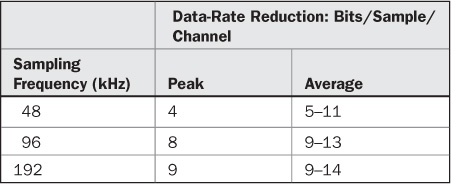
TABLE 11.2 MLP compression of a two-channel signal is relatively more efficient for higher sampling frequencies.

MLP supports all standard sampling frequencies and quantization may be selected for 16 to 24 bits in single-bit steps. MLP can code both stereo and multichannel signals simultaneously. The degree of compression varies according to the nature of the music data itself. For example, without compression, 96-kHz/24-bit audio consumes 2.304 Mbps per channel, thus a 6-channel recording would consume 13.824 Mbps. This would exceed, for example, the DVD-Audio maximum bit rate of 9.6 Mbps. Even if the high bit rate could be recorded, it would allow only about 45 minutes of music on a single-layer DVD-Audio disc with a capacity of 4.7 Gbytes. In contrast, MLP would allow 6-channel 96-kHz/24-bit recordings. It may achieve 38 to 52% of bandwidth reduction, reducing bandwidth to 6.6 Mbps to 8.6 Mbps, allowing a playing time of 73 to 80 minutes on a DVD disc. In the highest quality DVD-Audio two-channel stereo mode of 192-kHz/24-bit, MLP would provide a playing time of about 117 minutes, versus a playing time of 74 minutes for PCM coding.

Generally, more compression is achieved with higher sampling rates such as 96 kHz and 192 kHz, and less compression is achieved for lower sampling rates such as 44.1 kHz. This is shown in Table 11.2. Data-rate reduction is measured in bit/sample/channel, both in peak and average rates, where peak rates reflect performance on signals that are difficult to encode. In this table, for example, a peak-data rate reduction of 9 bits/sample means that a 192-kHz 24-bit channel can be coded to fit into a 24 − 9 = 15-bit PCM channel. The peak-rate reduction is important when encoding for any format because of the format’s bit-rate channel limit. The average-rate reduction indicates the average bit savings and is useful for estimating the storage capacity needed for archiving, mastering, and editing applications. For example, a 192 kHz 24-bit signal might be coded at an average bit rate of 24 − 11.5 = 12.5 bits per channel. This table shows examples of compression for a two-channel recording. Compression increases if the number of channels increases, if channels are correlated, if any of the channels have a low bandwidth, and if any of the channels are lightly used (as with some surround channels). With MLP, the output peak rate is always reduced relative to the input peak rate.

MLP supports up to 63 audio channels, with sampling frequencies ranging from 32 kHz to 192 kHz and word lengths from 14 to 24 bits. Any word length shorter than 24 bits can be efficiently transmitted and decoded as a 24-bit word by packing zeros in the unused LSBs, without increasing the bit rate. Moreover, this is done automatically without the need for special flagging of word length. In addition, mixed sampling frequencies and word lengths are also automatically supported. The MLP core accepts and delivers PCM audio data; other types of data such as low-bit, video, or text cannot be applied to the encoder.

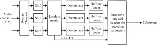
FIGURE 11.25 An example of an MLP encoder showing a lossless matrix, decorrelators, and Huffman coders. (Stuart, 1998b)

MLP does not discard data during coding; instead, it “packs” the data more efficiently. In that respect, MLP is analogous to computer utilities such as Zip and Stuffit that reduce file sizes without altering the contents (algorithmically, MLP operates quite differently). Data reduction aside, MLP offers other specific enhancements over PCM. Whereas a PCM signal can be subtly altered by generation loss, transmission errors, and other causes as it passes through a production chain, MLP can ensure that the output signal is exactly the same as the input signal by checking the MLP-coded file and confirming its bit accuracy.

The MLP encoder inserts proprietary check data into the bitstream; the decoder uses this check data to verify bit-for-bit accuracy. The bitstream is designed to be robust against transmission errors from disc defect or broadcast breakup. Full restart points in the bitstream occur at intervals of between 10 ms to 30 ms, when the content is easy to compress, and hard to compress, respectively. Errors cannot propagate beyond a restart point. Following a dropout, lossless operation will resume. MLP uses full CRCC checking and minor transmission errors are recovered in less than 2 ms. Recovery from a single bit error occurs within 1.6 ms. Full recovery from burst errors can occur within 10 ms to 30 ms; recovery time may be longer (36 ms to 200 ms) for a simple decoder. Interpolation may be used to prevent clicks or pops in the audio program. The restart points also allow fast recueing of the bitstream on disc. Startup time is about 30 ms and is always less than 200 ms (for complex passages that are difficult to compress). Similarly, fast-speed reviewing of audio material can be accommodated.

MLP applies several processes to the audio signal to reduce its overall data rate, and also to minimize the peak data rate in the variable rate of output data. A block diagram of the encoder is shown in Fig. 11.25. Data may be remapped to expedite the use of substreams. Data is shifted to account for unused capacity, for example, when less than 24-bit quantization is used or when the signal is not full scale. A lossless matrixing technique is used to optimize the data in each channel, reducing interchannel correlations. The signal in each channel is then decorrelated (inter-sample correlation is reduced) using a separate predictor for each channel. The encoder makes an optimum choice by designing a decorrelator in real time from a large variety of FIR or IIR prediction filters (this process takes into account the generally falling high-frequency response of music signals) to code the difference between the estimated and actual signals. A separate predictor is used for each encoded channel. Either IIR or FIR filters, up to 8th order, can be selected, depending on the type of audio signal being coded. MLP does not make assumptions about data content, nor search for patterns in the data. The decorrelated audio signal is further encoded with entropy coding to more efficiently code the most likely occurring successive values in the bitstream. The encoder can choose from several entropy coding methods including Huffman and Rice coding, and even PCM coding. Multiple data streams are interleaved.

The stream is packetized for fixed or variable data rate. (Data is encoded in blocks of 160 samples; blocks are assembled into packets and the length of packets can be adjusted, with a default of 10 blocks, or 1600 samples.) A first-in, first-out (FIFO) buffer of perhaps 75 ms is used in the encoder and decoder to smooth the variable data rate. To allow more rapid startup, the buffer is normally almost empty, and fills when the look-ahead encoder determines that a high entropy segment is imminent. To account for this, the decoder buffer empties. This helps to maintain the data rate below a preset limit, and to reduce the peak data rate.

Because data is matrixed into multiple substreams, each buffered separately, simple decoders can access a subset of the signal. MLP can use lossless matrixing of two sub-streams to encode both a multichannel mix and stereo downmix. Downmix instructions determine some coefficients for the matrices and the matrices perform a transformation so that two channels on one substream decode to provide a stereo mix, and also combine with another substream to provide a multichannel mix. Thus, the addition of the stereo mix adds minimal extra data, for example, one bit per sample.

The MLP bitstream contains a variety of data in addition to the compressed audio data. It also contains instructions to the decoder describing the sampling rate, word length, channel use, and so on. Auxiliary data from the content provider can describe whether speaker channels are from hierarchical or binaural sources, and can also carry copyright, ownership, watermarking data, and accuracy warranty information. There is also CRCC check data, and lossless testing information.

A fixed bit rate can be achieved in a single-pass process if the target rate is not too severe. When the desired rate is near the limit of MLP, a two-pass process is used in which packeting is performed in a second pass with data provided by the encoder. In any case, a fixed bit rate yields less compression than a variable bit rate.

A fixed rate gives predictable file sizes, allows the use of MLP with motion video, and ensures compatibility with existing interfaces. A specific bit rate may be manually requested by the operator. To achieve extra compression, for example, to fit a few more minutes onto a disc data layer, small adjustments may be made to the incoming signal. For example, word length could be reduced by one bit by requantizing (and redithering and perhaps noise shaping) a 24-bit signal to 23 bits. Alternatively, a channel could be lowpass-filtered, perhaps from 48 kHz to 40 kHz. MLP also allows mixed stream rates in which the option of a variable rate accompanies a fixed-stream rate.

An MLP transcoder can re-packetize a fixed-rate bitstream into a variable-rate stream, and vice versa; this does not require encoding or decoding. Editing can be performed on data while it is packed in the MLP format. The MLP decoder automatically recognizes MLP data and reverts to PCM when there is no MLP data. Different tracks can intermingle MLP and PCM coding on one disc. Finally, MLP is cascadable; files can be encoded and decoded repeatedly in cascade without affecting the original content.

MLP is optionally used on DVD-Audio and Blu-ray titles. The MLP bitstream can also be carried on AES3, S/PDIF, IEEE 1384, and other interconnections. MLP was largely developed by Robert Stuart, Michael Gerzon, Malcolm Law, and Peter Craven.

Other lossless codecs have been developed. These codecs include FLAC (Free Lossless Audio Codec), LRC (Lossless Real-time Coding), Monkey’s Audio, WavPack, LPAC, Shorten, OptiFROG, and Direct Stream Digital (used in SACD). A lossless WMA codec is part of the Windows Media 9 specification. ALS (Audio Lossless Coding) is used in MPEG-4 ALS. The FLAC lossless codec is free, open-source, and can be used with no licensing fees. FLAC can support PCM samples with a word length from 4 to 32 bits per sample, a wide range of sampling frequencies, and 1 to 8 channels in a bit-stream. FLAC is available at http://flac.sourceforge.net. FLAC is free for any commercial or noncommercial applications.