CHAPTER 18
Sigma-Delta Conversion and Noise Shaping

Design limitations and the relative cost of PCM converter architectures encouraged the development of sigma-delta converters. These converters are characterized by short word lengths, very high oversampling rates, and noise shaping. They demonstrate that conversion can be performed either with a high-resolution quantizer at a low sampling rate (as in traditional converters), or with a low-resolution quantizer at a high sampling rate (as in sigma-delta converters). Sigma-delta analog-to-digital (A/D) and digital-to-analog (D/A) converters both use conversion methods such as sigma-delta modulation with noise shaping, and process high sampling-rate signals with oversampling and decimation filters. These converters share the goal of translating nonideal converter errors into uncorrelated, benign noise. Sigma-delta converters are sometimes referred to as one-bit or multi-bit converters, depending on the specific architecture employed. In addition, nonoversampling noise shaping is critical when reducing word length during a data transfer, for example, when transferring a 24-bit master recording to a 16- or 20-bit format.

Sigma-Delta Conversion

Conversion of PCM audio data words, using a resistor ladder, is a traditional approach. A PCM system represents the analog waveform as an amplitude signal, storing information that measures the amplitude sample by sample. However, the method is flawed when quantization introduces differential nonlinearity errors in the amplitude representation. Moreover, because a multiplicity of bits are used to form the representation, and because each bit has an error unequal to the others, the overall error varies with each sample, and is thus difficult to correct. In practice, calibration procedures during manufacture, and sophisticated circuit design are required to achieve high performance. Understandably, manufacturers sought to develop alternative conversion methods, including sigma-delta converters. Sigma-delta methods are particularly desirable for A/D conversion because they obviate the need for an analog brick-wall anti-aliasing filter. But the method also offers many advantages in D/A conversion, particularly when designing a mixed-signal integrated circuit that combines A/D, D/A, and DSP functions.

It is not easy to see how one bit (or a few) can replace 16 or more bits. Consider this analogy: traditional ladder converters are like a row of light bulbs, each connected to a switch. Sixteen bulbs, for example, each with a different brightness, can be lighted in various combinations to achieve 2¹⁶ or 65,536 different brightness levels. However, relative differences in individual bulb intensities will introduce error into the output brightness level. Any particular switch combination may not exactly produce the desired brightness. Similarly, ladder converters introduce error as they attempt to reproduce the audio signal.

Sigma-delta technology uses a wholly different approach. Instead of many bulbs and switches, only one bulb and one switch are used. Brightness is varied by simply switching the bulb on and off. For example, if the bulb is dynamically switched on and off equally, the output is at half-brightness. If the bulb’s on-time is increased, brightness will increase. Similarly, sigma-delta converters may ideally use one bit to represent audio amplitude, with very fast switching and very accurate timing. Sigma-delta technology is an inherently precise way to represent an audio waveform.

PCM conversion divides the signal in multiple amplitude steps. However, sigma-delta conversion divides the signal in time, keeping amplitude changes constant. Non-intuitively, a high- or low-level pulse signal can represent an audio signal. For example, pulse-density modulation (PDM) can be used. Fig. 18.1 shows how a single constant-width pulse, with either a high or low level, can reconstruct a waveform. Alternatively, a pulse-width modulation (PWM) signal can be used to reconstruct the output signal (variations are pulse-edge and pulse-length modulation).

Sigma-delta converters are called one-bit converters when one quantized audio bit is output, and called multi-bit converters when the audio signal is quantized to several bits (perhaps four). True one-bit sigma-delta converters output full-scale positive or negative pulses that ensure perfect linearity. However, their inherently coarse quantization yields a higher noise floor. Thus, higher orders of noise shaping are required for good in-band dynamic range performance. In addition, one-bit converters are susceptible to phase jitter on the modulator clock. Relatively small jitter levels can yield a full-scale error in the one-bit signal. Multi-bit sigma-delta converters use multiple quantization levels and this yields a relatively lower noise floor both in-band and out of band. This allows the use of a relatively lower oversampling ratio, as well as lower-order noise shaping. In addition, the smaller quantization levels of multi-bit converters make them more tolerant of phase jitter. However, care must be taken to achieve good linearity. Generally, multi-bit sigma-delta converters are employed in higher-quality audio applications.

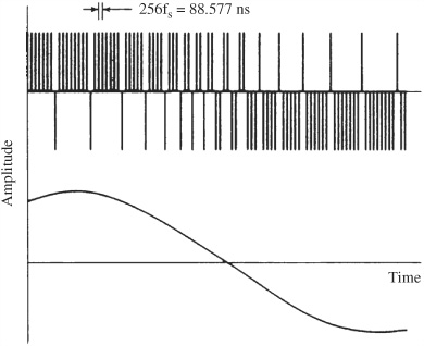
FIGURE 18.1 Pulse-density modulation can be used to code and reconstruct an analog waveform.

One-bit sigma-delta converters are inherently linear; any level mismatch results in an offset. However, multi-bit sigma-delta converters can have element mismatches that result in noise and distortion. In this architecture, a capacitor or resistor element is assigned to a fixed code; small variations yield a mismatch. For example, assuming 32 elements, a 1% mismatch yields about 0.1% THD + N distortion. The distortion is also signal-dependent. To address this mismatch, codes can be used to randomly assign different elements in each cycle, but this increases noise. Assuming 32 elements and an oversampling ratio of 128, a 1% mismatch would yield a dynamic range of only 80 dB. Dynamic element matching (DEM) is a common solution used to reduce the effect of mismatch errors in the conversion elements of multi-bit converters. With DEM, analog capacitor elements are swapped so that the mismatch error is averaged close to zero. DEM can use open-loop noise shaping after the modulator to convert the error into low-level benign noise. For example, elements can be selected cyclically, depending on the weighting of the input data. This averages the mismatch, and the noise from mismatching is first-order noise shaped. In other designs, the mismatch shaping function can be placed inside the sigma-delta feedback loop. The randomized errors are shaped by the modulator, further reducing the in-band level. Assuming 32 elements and an oversampling ratio of 128, a 1% mismatch would yield a dynamic range of 120 dB.

Sigma-delta conversion methods are widely used in digital audio products. These techniques are extremely competitive in both A/D and D/A applications because they obviate the need for analog brick-wall filters. Although sigma-delta methods use familiar techniques such as oversampling, highly sophisticated processing is required to implement noise shaping and thus decrease the high in-band noise levels otherwise present in sigma-delta conversion. A variety of sigma-delta A/D and D/A architectures have been devised, with different algorithms and orders of noise shaping.

Delta Modulation

In PCM a signal is sampled and quantized into discrete steps; the maximum signal amplitude determines the maximum quantizer range. Traditional PCM A/D and D/A converters are shown in Fig. 18.2A. Quantization error is uniformly present across the Nyquist frequency band from 0 to f_s/2 Hz and cannot be removed from the signal; f_s is the sampling frequency. If quantization is performed at a higher sampling frequency R × f_s Hz where R is the oversampling rate, the error is spread across the band to R × f_s/2 Hz, hence the noise in the audio band is reduced by 3 dB for every factor of 2 oversampling.

With a maximum-amplitude sinusoidal input signal, oversampling will increase the signal-to-error ratio as follows:

S/E = 6.02(N + 0.5L) + 1.76 dB

where N = the number of quantization bits

L = the number of octaves of oversampling

For example, an oversampling A/D converter can perform as well as a longer word length A/D converter, yielding a benefit of 0.5 bit/oversampling octave. However, the benefit is limited. For example, a 10-bit improvement would require an L of 20 octaves, equivalent to an impossible oversampling factor of 1 million. It is the aim of noise shaping to introduce a highpass function in the noise spectrum and thus improve oversampling performance.

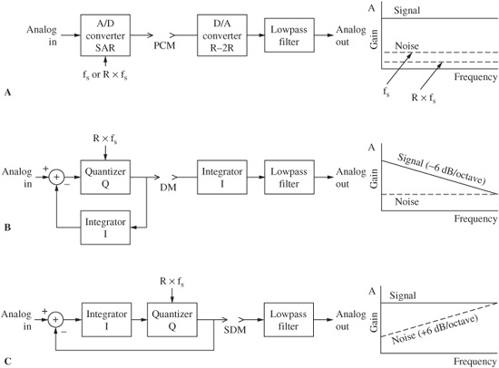
FIGURE 18.2 A comparison of modulation methods used in A/D and D/A conversion. A. Pulse-code modulation (PCM) yields a flat signal and noise floor. B. Delta modulation (DM) yields a signal that falls with frequency. C. Sigma-delta modulation (SDM) yields a noise floor that rises with frequency.

Delta modulation and sigma-delta modulation (also called delta-sigma) were developed in the 1940s and 1960s, respectively, for voice telephony applications. Limitations prohibited their use in high-quality music applications until the emergence of high-speed digital signal processing techniques in the 1980s, that improved audio performance. Differential pulse-code modulation (DPCM) is a technique in which the derivative of the signal is quantized. When signal changes between sample periods are small, the quantizer’s word length can be reduced. With very high oversampling rates, the changes between sample periods are made very small, thus the quantizer can be reduced to one bit. A one-bit DPCM coder is known as a delta modulator (DM). In other words, DM codes the differences in the signal amplitude, its slope, instead of the signal amplitude itself. In contrast, a sigma-DPCM technique places an integrator at the input to the quantizer. Instead of coding the slope of the signal, sigma-DPCM, like PCM, codes its amplitude. However, with sigma-DPCM, the signal can be quantizing to only one or a few bits; both implementations are generally known as sigma-delta modulation. As with delta modulation, sigma-delta modulation requires high oversampling rates.

A delta-modulation encoder and decoder are shown in Fig. 18.2B; this is known as a single integration modulator. The analog input signal is compared to the integrated output pulses and the delta (difference) signal is applied to the quantizer. The quantizer generates a positive pulse when the difference signal is negative, and a negative pulse when the difference signal is positive. This difference error signal moves the integrator step by step closer to the present value input, tracking the derivative of the analog input signal. The integrator’s output is a past approximation to the input, thus the coder operates similarly to other integrating feedback loops such as phase-locked loops.

A delta-modulation decoder consists of an integrator and a lowpass filter. When the one-bit pulses are integrated using a time constant that is long compared to the sample period, a step waveform is produced. An output analog waveform is produced by low-pass filtering this step waveform. Requantization error at the output of the integrator is white. As in PCM, oversampling decreases the error level by 3 dB for every factor of two oversampling. The dynamic range can be improved, that is, the requantization error made smaller, by making the delta (difference or step size) value smaller. The limit to which the delta can be reduced is given by the maximum derivative of the signal. The coded signal amplitude decreases at 6 dB/octave; thus, S/N decreases as the signal frequency increases.

The maximum derivative occurs at maximum signal frequency and maximum signal amplitude. Exceeding this limit causes slope overload distortion. For music signals, the delta value must be high, resulting in a high quantization error level. When the signal has reduced high-frequency content, as in speech, delta can be reduced. In any case, the success of DM hinges on assumptions about the nature of the encoded signal. This dependence of the dynamic range on the signal spectrum, and good performance only when the signal has lowpass characteristics, as well as correlated patterns at low signal levels, limits single-integration DM applications.

To convert a maximum amplitude 16-bit word, a one-bit modulator would have to perform 2¹⁶ toggles per conversion period. With a sampling frequency of 44.1 kHz, this would demand an unrealistic toggle rate of approximately 2.9 GHz. As the rate is slowed to accommodate hardware limitations, noise levels increase to an intolerable level. Looked at in another way, bit reduction at a high sampling frequency is required to output a one-bit signal from a high-bit source; this greatly degrades the signal’s dynamic range.

Sigma-Delta Modulation

Sigma-delta modulation (SDM) was developed to overcome the limitations of delta modulation. Sigma-delta systems quantize the delta (difference) between the current signal and the sigma (sum) of the previous difference. A first-order (single integration) sigma-delta modulation encoder and decoder are shown in Fig. 18.2C. An integrator is placed at the input to the quantizer; signal amplitude is constant with increasing frequency. The input to the midrise quantizer is the integral of the difference between the input and the quantized output as applied via negative feedback. If the input signal in one sample period is greater than the value accumulated in the feedback loop over previous samples, the converter outputs a “1.” Otherwise, if it is lower, the output is a “0.” In other words, the difference between the input signal and the accumulated error is quantized. When the error is sufficiently large, the quantizer changes state to reduce the error. Thus, the difference between the input signal and the output signal approaches zero; the average value of the output approximates the input. There is little dc error in the output signal. However, the frequency spectrum of the quantizing error rises with increasing frequency (6 dB/octave).

The integrator forms a lowpass filter on the difference signal thus providing low-frequency feedback around the quantizer. This feedback results in a reduction of quantization noise at low (in-band) frequencies. Unlike PCM and DM, the noise floor is not flat, but shaped by a first-order highpass characteristic as analyzed below. In practice, the in-band noise floor level is not satisfactory with first-order sigma-delta modulation. In addition, quantization noise is highly correlated in a first-order modulator. Further noise shaping must be achieved with higher-order (multiple integration) sigma-delta modulation coders. Michael Gerzon and Peter Craven have shown that shaped noise in multi-bit noise shapers will occupy equal areas above and below the original noise level. Since this relationship occurs on a logarithmic vertical axis and linear frequency axis, shaping increases the total noise power. The benefit, of course, is lower in-band noise.

Like PCM, sigma-delta modulation quantizes the signal amplitude directly, and not its derivative as in DM. Thus the maximum quantizer range is determined by the maximum signal amplitude and is not dependent on signal spectrum. As with delta modulation, to achieve high resolution, high oversampling rates are required. For example, with an audio band of 24 kHz and 64 times oversampling, the internal sampling frequency rises to 3.072 MHz, thus quantization noise is spread from dc to 1.536 MHz. However, because the quantizer has only two states, the quantization error, and the resulting noise level, is high. To overcome this, sigma-delta modulators add noise shaping to move the noise power to higher, out-of-band frequencies. The noise is shaped by the inverse of the loop transfer function; when a lowpass filter is placed in the loop, the noise spectrum increases with frequency. In many designs, a multi-bit quantizer is used within the loop and a low-bit PCM signal is coded; the dynamic range increases with 6 dB for every quantization bit. As in one-bit designs, the noise floor increases by 6 dB/octave in multi-bit designs, and noise shaping is required.

A one-bit sigma-delta modulation decoder theoretically requires only a lowpass filter to decode the signal, to remove high-frequency (out-of-band) components. In other words, it averages the output signal to produce an analog waveform. An integrator is not needed in the decoder (as in DM) because the signal’s amplitude is coded, not its slope. In multi-bit designs, a D/A converter is needed in the decoder to decode the low-bit PCM signal.

Analysis of a First-Order Sigma-Delta Modulator

The signal and noise transfer functions for a first-order sigma-delta modulator are analyzed in Fig. 18.3. X(z) is the z-transform of the input sequence and Y(z) represents the output sequence. The quantization error is represented as white noise N(z). For a zero noise source, the transfer function shows a lowpass characteristic. For a zero signal, the transfer function shows a highpass characteristic. In other words, as the loop integrates the difference between the input signal and the sampled signal, it lowpass filters the signal and highpass filters the noise. If the system is designed so the signal’s frequency content is less than the filter’s cutoff frequency, the signal will not be affected. Given a first-order noise-shaping loop, with a maximum amplitude sinusoidal input, the maximum signal-to-error ratio will be:

S/E = 6.02(N + 1.5L) −3.41 dB

where N = the number of quantization bits

L = the number of octaves of oversampling

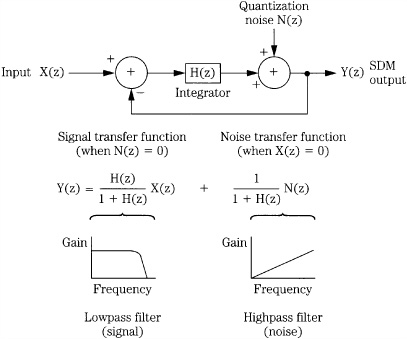
FIGURE 18.3 A z-transform analysis of a sigma-delta modulator. (Hauser, 1991)

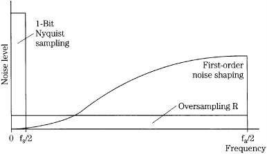
FIGURE 18.4 With one-bit conversion, quantization noise is quite high. In-band noise is reduced with oversampling. With noise shaping, quantization noise is shifted away from the audio band, further reducing in-band noise.

For example, an A/D converter with sigma-delta first-order noise shaping provides a benefit of 1.5 bits/octave compared to an oversampling converter without a noise-shaping loop.

The performance of a sigma-delta converter relies on both oversampling, and its noise-shaping characteristic. The quantization noise floor falls from 0 to f_s/2 Hz and is quite high, as shown in Fig. 18.4. Quantization noise is reduced with an R oversampling ratio because noise is spread over a 0-Hz to f_a/2-Hz spectrum where f_a = R × f_s Hz. With sigma-delta noise shaping, in-band noise (0 to f_s/2) is further decreased and out-of-band noise is increased.

Figure 18.5 summarizes the mathematical basis of first-order sigma-delta noise shaping. Quantization noise is assumed to be random, and the quantizer is modeled as an additive noise source. Note that the (1 − z⁻¹) factor doubles quantized noise power; however, the same factor also shifts the noise to higher frequencies. This sigma-delta modulator forms the basis for many A/D and D/A one-bit and multi-bit converters.

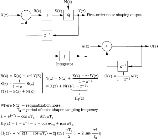
FIGURE 18.5 Analysis of a first-order sigma-delta noise shaper.

Higher-Order Noise Shaping

As noted, first-order (single integration) sigma-delta modulation is not satisfactory for high-fidelity audio performance. Higher-order loops further decrease in-band quantization noise, with the penalty of increased total noise power. For example, a second-order loop would yield:

S/E = 6.02(N + 2.5L) − 11.14 dB

This provides a benefit of 2.5 bits/octave, with a fixed-noise penalty approximately equal to two equivalent bits.

The input/output characteristic of a basic sigma-delta noise shaper of nth order is:

Y(z) = X(z) + (1 − z^⁕1)ⁿ N(z)

where Y(z) = the noise-shaped output

X(z) = the input signal

n = the order of the differentiation

N(z) = the quantization noise (assumed to be white)

This characteristic can be theoretically composed of n cascaded digital differentiators. As n increases, the slope in frequency of the shaping function increases, thus it is more effective in suppressing low-frequency noise. However, the out-of-band noise could overly burden subsequent analog filters. A successful noise-shaping circuit thus seeks to balance a high oversampling rate with noise-shaping order to reduce in-band noise and shift it away from the audible range. Higher-order noise-shaping loops can remove even more in-band noise overall, but relatively more noise is present near the Nyquist frequency. Hence these algorithms are more effective at high oversampling rates so there is more spectral space between the highest audio frequency and the Nyquist frequency; this allows the use of very simple analog lowpass filters.

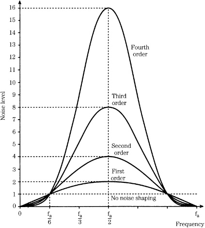
FIGURE 18.6 Higher orders of noise shaping result in more pronounced shifts in requantization noise.

Using first-order and higher-order noise-shaping algorithms, a series of noise-shaping curves can be generated, as shown in Fig. 18.6. As higher orders of noise shaping are used, the in-band noise level is decreased. The frequency response curves described by sigma-delta noise-shaping equal a unity value at f_a/6 Hz where f_a is the noise-shaping oversampling frequency. Noise is reduced only for f < f_a/6 Hz, and increased for f_a/6 < f < f_a/2 Hz. The noise level reaches a maximum at f_a/2 Hz. As the oversampling rate is increased, the portion of the noise curve in the audio band is relatively reduced. Although the shape of the noise curve remains the same, high oversampling rates relatively decrease in-band noise.

In a traditional noise-shaper design, the poles of the loop filter are at 0 Hz, as in an ideal integrator; this results in zeros in the audio band. In some noise-shaper designs, a technique called zero-shifting is used to modify the rising noise spectrum by shifting one or more zeros to the edge of the audio band (for example, 18 kHz). For example, when two zeros are shifted in a third-order noise filter, noise in the range from 13 kHz to 20 kHz can be reduced, but increased below 13 kHz. Overall, the noise measurement is enhanced. However, suppression of idle patterns and thresholding effects can be diminished; thus, the zero-shifting technique must be used with care.

Idle Tones and Limit Cycles

The low-level linearity of low-order (particularly first-order) sigma-delta noise-shaping algorithms can be degraded by idle tones. The quantization noise is not always random, and instead can be correlated to the input signal. This is an idle tone, a high-frequency oscillation of the modulator output. Given a zero input signal, a noise shaper can output an alternating 1010 pattern. A very low-level input might result in a similar 1010 pattern, but disturbed by double 1s and 0s. If the period of the repetition of such patterns is long enough, they yield energy that might fall in the audio baseband, being audible as a deterministic or oscillatory tone, rather than as noise. Because they occur when the channel is idling, these nonlinear patterns are called idle tones, or idling patterns, and result in idle channel noise. The double codes will be generated, or not, depending on the duration of the input signal. The phenomenon is especially characteristic of low-amplitude, high-frequency sine waves. Because the phenomenon has a frequency-dependent threshold level, below which the signal is not coded, the effect is sometimes called thresholding.

First-order sigma-delta noise shapers particularly exhibit these effects because of their stable 1010 patterns. Higher-order noise shapers are much less prone to the problem because their output patterns are less stable. Thus, for example, virtually all sigma-delta converters use at least a second-order modulator loop. However, in many multistage designs, the effect can occur in each of the cascaded low-order stages. Thus, it is important to add a dither signal in the first stage to disturb any fixed patterns and remove the correlation. Dither is applied most effectively in multi-bit converters, and less effectively in true one-bit converters. Generally, multi-bit converters are completely linearized with triangular pdf dither, which eliminates noise modulation but slightly increases the level of the noise floor. It is felt that true one-bit converters cannot be fully dithered because this would overload the modulator. In true one-bit converters, dither has both advantages and disadvantages and the optimum dithering technique has not yet been found; other methods are sometimes used to linearize the converter.

A limit cycle is a repeating output sequence. It will yield spurious spectral lines and potentially audible distortion on the output. Limit cycles may occur even in simple noise shapers for some input signals such as a dc input. Their occurrence also depends on the initial state of the noise-shaper filter. Limit cycles can generally be avoided by adding sufficient dither. For example, high-order noise shapers can use small dither levels, such as a rectangular pdf dither with a peak-to-peak amplitude of 0.01 LSB.

Higher-order sigma-delta modulation loops offer wider dynamic range and overall better performance, but loops greater than second-order can be unstable. The quantizer is nonlinear because its effective “gain” inversely varies with the input level. A large input signal can overload the loop, reducing the gain of the quantizer, thus causing instability that will persist even after the signal is withdrawn. For example, a powering-up transient could cause a converter to oscillate. Converters thus sense instability by counting the number of consecutive ones or zeroes in the bitstream, and reset when necessary.

One-Bit D/A Conversion with Second-Order Noise Shaping

A sigma-delta D/A converter comprises a digital interpolation filter, sigma-delta modulator, one-bit or multi-bit converter, and a low-order lowpass output filter. The input digital word, with long word length, is applied to the interpolation filter that lowpass filters the signal and increases its sampling rate with oversampling. The digital modulator noise-shapes the signal and reduces the word length to one or a few bits. For example, its transfer function can be implemented with an IIR filter. The signal is effectively lowpass-filtered and the quantization noise is highpass-filtered. The analog output filter removes the high-frequency shaped quantization noise as well as high-frequency images.

One implementation of a true one-bit D/A conversion method comprises an over-sampling filter, second-order sigma-delta noise shaping, and pulse-density modulation (PDM) output. The sampling frequency is increased from 44.1 kHz to 11.2896 MHz, an increase of 256 times. At the same time, the 16-bit signal is converted to a one-bit signal that reconstructs the audio waveform. The requantization error of the output signal is corrected by feedback. Instead of outputting a signal with conventional quantization error, the error undergoes sigma-delta processing to attenuate its in-band level.

The output bit, operating at a frequency of 11.2896 MHz, is converted to an analog signal using a simple switched capacitor network. Specifically, a capacitor is charged and discharged according to the 1 or 0 value of the data. The result is an analog waveform that reflects the encoded waveform through time-averaging of the output bit. The network’s operation is accurate, and hence the error of the signal is low. There are only positive and negative full-scale reference points. Errors in the reference values will generate a gain offset error, but not a linearity error. The offset error can easily be removed. In practice, nonlinearities could result from idle patterns in the noise-shaping circuitry.

Figure 18.7 represents the operation of a one-bit PDM converter. It performs noise shaping through feedback loops and generates a one-bit signal for conversion to analog. The noise shaper consists of two integration (filter) loops to reduce in-band requantization noise. The output (H) of the quantizer is +1 if its input is positive (MSB = 0), and −1 if its input is negative (MSB = 1); the one-bit code output from the quantizer is simply a sign bit. Following a limiting operation designed to prevent overflow, the remainder of each sample is fed back as a quantization error. The error signal (I) is fed back into the double integration loops. Values inside the loop exceed the unit value; in other words, wider data buses are required. In this case, a 21-bit data bus is used within the loop; signals are processed in two’s complement form.

Also, if large values are input to the circuit, the limiter would be needed to prevent overloading of the loops. Ideally, with no input signal, the coder should output only a tone at R × f_s/2 Hz where R is the oversampling rate. However, idle tones can also occur at additional frequencies. To overcome this, dither can be added to the input data so the circuit always operates with a changing signal even when the audio signal is zero or dc.

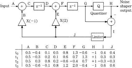
FIGURE 18.7 Operation of a second-order noise-shaping circuit.

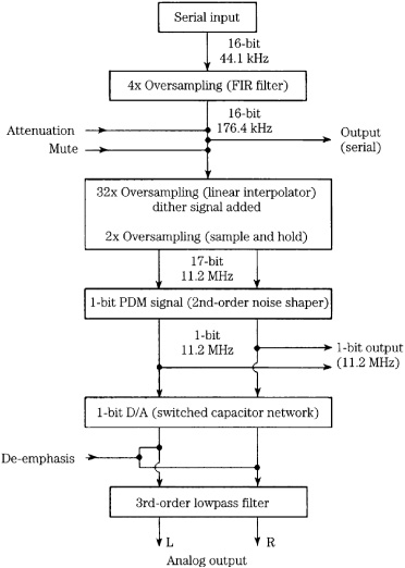
FIGURE 18.8 Processing elements in a second-order, pulse-density modulation D/A conversion system.

Figure 18.8 shows the complete system, including the one-bit PDM noise-shaper modeled above. The first of the three oversampling stages performs four-times over-sampling to attenuate image spectra; in addition, first-order noise shaping is performed in the filter. The second stage performs 32-times oversampling. A dither signal (–20 dB at 352 kHz) is added to prevent idle tones from causing nonlinearity. Two-times oversampling is performed in the third stage. This 17-bit signal (dither adds one bit to the original 16-bit signal) undergoes second-order noise shaping as described above, and a single bit is output from the quantizer. Finally, D/A conversion is accomplished at a one-bit D/A converter via pulse-density modulation that outputs two-valued (±) data at 256-times oversampling, or 11.2896 MHz. A third-order analog lowpass filter removes out-of-band high-frequency components.

The output signal conveys the audio waveform through the density of pulses above and below zero (see Fig. 18.1); this pulse-density modulation signal is converted to an analog signal using a switched dual-capacitor network. Two control signals representing the data stream’s logic 0 and logic 1 values control the switching of the capacitors, subject to a clock pulse. During the negative half of the clock, the first capacitor discharges while the second capacitor charges. During the positive half, if the data is 1, the first capacitor is charged by taking a fixed amount of charge from the summing node of an operational amplifier. If the data is 0, a fixed charge is transferred into the summing node from the second capacitor. In this way, there are only positive and negative full-scale reference points, and intermediate points are determined by time averaging. There is no MSB change around zero, for example, because zero is represented by an equal number of positive and negative full-scale pulses. Zero-cross distortion is thus eliminated.

In this one-bit converter, the quantization noise introduced by the word length reduction is spectrally shaped by a lowpass feedback loop around the quantizer (see Fig. 18.7). Second-order noise shaping is performed:

where Y(z) = the noise-shaped output

X(z) = the input signal

N(z) = the quantization noise

The requantization noise of the output signal is corrected by feedback, and noise shaping attenuates its in-band level. As a result, the spectrum of the noise in the output signal is shifted away from the audio band. Figure 18.9 summarizes the mathematical basis of second-order noise shaping.

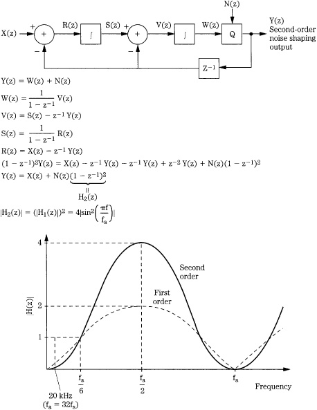
FIGURE 18.9 Analysis of a second-order noise shaper.

Multi-Bit D/A Conversion with Third-Order Noise Shaping

When the noise-shaping circuits in sigma-delta modulators exceed second order, the noise-shaping feedback loops can pose overload or oscillation problems. For example, an overload would effectively reduce the magnitude of loop gain, lowering the crossover frequency, where phase shift is too large for stability. When a loop filter H(z) has three or more integrations, its phase shift can be 180° at the frequency where the loop gain magnitude reaches unity at the crossover frequency.

Higher-order noise shapers overcome this problem with a more complex loop architecture that often uses multistage noise shaping. The loop filter H(z) provides a high-order lowpass response at low baseband frequencies, but gain drops to a first- or second-order lowpass response nearer the crossover frequency. This approach provides good in-band noise shaping, with sufficient conditional stability.

The MASH system is a multistage third-order noise-shaping method. It is an example of a practical multi-bit converter. One implementation of this design accepts 16-bit words at a nominal sampling frequency, and a digital filter performs eight-times oversampling and outputs 24-bit words. Noise-shaping circuits output 11-valued data, at a 32-times oversampling rate. D/A conversion is accomplished via pulse-width modulation (PWM), outputting the data at a 768-times oversampling rate.

As noted, generally, if noise-shaping circuits exceed second-order they can be prone to oscillation from instability. To avoid such errors, this third-order implementation uses a multistage configuration. A simplified schematic for the complete noise shaper is shown in Fig. 18.10; it contains a first-order noise shaper in parallel with a second-order noise shaper. The input signal is applied to quantizer Q₁ after the error signal through the delay block is subtracted from the input. The signal output from the first loop is also applied to the second loop. The output of quantizer Q₂ is differentiated and added to the output of the first loop to form the final output signal. Thus, the requantization error of the first loop is requantized by the second, and canceled by adding the requantized noise to the first loop’s signal. The outputs of each stage can be characterized as:

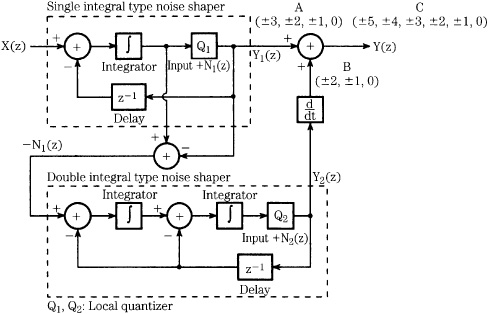
FIGURE 18.10 A multistage third-order noise-shaping circuit with output of 11 data values before PWM reconstruction.

where Y₁(z) and Y₂(z) = the outputs of stages 1 and 2, respectively

X(z) = the input signal

N₁(z) and N₂(z) = quantization noise of the local quantizers Q₁ and Q₂, respectively

When both sides of the second equation are multiplied by (1 − z⁻¹) and this is added to the first equation, observe that the quantization error of the first stage can be canceled. By passing the output of the second stage through a differentiator and adding it to the output of the first stage, the overall circuit output is:

In other words, the quantization error N₂(z) is output with a third-order differential characteristic (18 dB/octave), achieving reduced in-band noise compared to first- and second-order characteristics.

Input data is linearly requantized into a multi-bit output digital signal with seven values (±3, ±2, ±1, 0) at the main loop, and at the sub-loop the requantization error is requantized into five values (±2, ±1, 0). When these output values are added together, the digital signal output from the circuit represents 11 values (± 5, ± 4, ± 3, ± 2, ±1, 0). These different data values are shown graphically in Fig. 18.11. Using a vertical scale to represent amplitude of the values, it can be seen that the main loop outputs seven values of rough accuracy, and the sub-loop outputs five values with high-frequency content, used to eliminate the requantization error of the main loop. When summed, 11 values are output from the shaper to reconstruct the audio signal.

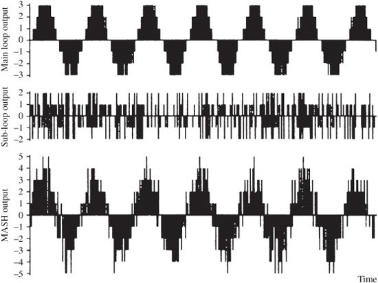
FIGURE 18.11 A graphical representation of the data values in a multistage noise shaper.

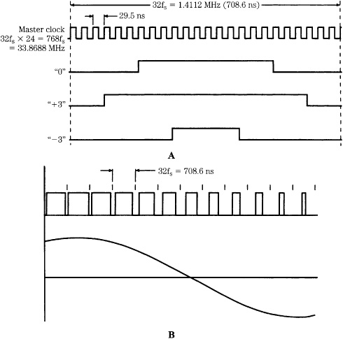
FIGURE 18.12 Pulse-width modulation data is output from a MASH converter. A. Examples of pulse-width modulation data. B. Reconstruction of the analog waveform.

The final element in the system is D/A conversion. The 11-valued signal is converted into pulses, each with a width corresponding to one value, as shown in Fig. 18.12A. This can be accomplished by applying the 4-bit output of the shaper to a lookup table to map 11 amplitude steps into 22 time steps with constant amplitude. For example, the figure shows the PWM waveforms resulting from the 0, +3, and −3 output values. In actuality, waveforms representing ±5, ±4, ±3, ±2, ±1, and 0 are all output. The widest pulses translate into a large positive output, and the narrowest pulses translate into a large negative output, as shown in Fig. 18.12B. The width of the pulses carries the vital information; the amplitude of this signal can only be high or low. At this point the signal has the form of PWM binary data. Because timing accuracy can be achieved through crystal oscillators, the widths are very accurate, and hence signal error is low.

The relatively coarse quantization permits accurate pulse timing by synchronizing pulse edges to the oversampling clock. Positive- and negative-going pulses are output, to cancel common noise. This 33.8688-MHz (768 × f_s) data forms a PWM representation of the waveform; Fig. 18.13 shows the spectrum of a 20-kHz input signal. Proof of performance can be evaluated by measuring the in-band noise of the system; it is below –100 dB. Figure 18.14 summarizes the mathematical basis of third-order noise shaping.

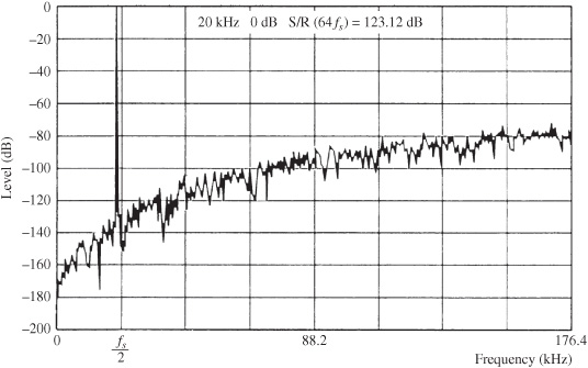
FIGURE 18.13 Reproduction of a 20-kHz waveform showing the effect of third-order noise shaping.

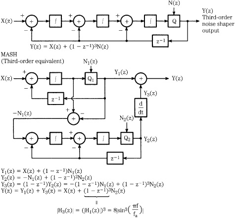
FIGURE 18.14 Analysis of a third-order noise shaper.

Multi-Bit D/A Conversion with Quasi Fourth-Order Noise Shaping

Victor Advanced Noise Shaping (VANS) is an example of a multi-bit D/A converter architecture using eight-times oversampling, a quasi fourth-order noise shaper, and pulse-edge modulation conversion. The noise shaper uses four loop filters in a configuration that yields in-band performance equivalent to fourth-order noise shaping. The VANS circuit is designed to operate like a fourth-order noise shaper at audible frequencies, gradually shifting toward second-order noise shaping at higher frequencies. This provides stability, yet improves performance in the audio band.

Thirty-two times oversampling is performed, and the output clock frequency is 16.9344 MHz (384 × f_s). With pulse-edge modulation, input data is converted into a binary pulse train with 15 discrete values (±7, ±6, ±5, ±4, ±3, ±2, ±1, 0). A differential configuration is used in which the rise of the leading edge of a pulse, and the fall of the trailing edge of a pulse, are output by two independent pulse-edge modulation converters. This determines the width of the pulse. Two converters output pulse trains based on the input signal, and an analog subtractor generates a composite signal determined by the leading and trailing edges of the pulse trains. This signal can take either a positive or a negative value. For example, data representing a −1 value would generate a short negative-going pulse, but data representing a +5 value would generate a longer positive-going pulse. When time averaged, these values create the analog waveform, as in pulse-width modulation. Figure 18.15 summarizes the mathematical basis of this quasi fourth-order noise shaping.

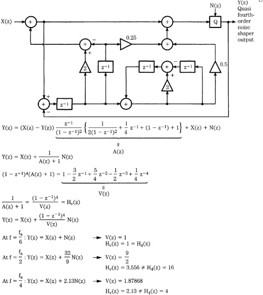
FIGURE 18.15 Analysis of a quasi fourth-order noise shaper.

Generally, even higher orders of noise shaping can be successfully employed, yielding very low in-band noise floors. For example, a fifth-order sigma-delta modulator is used in some Direct Stream Digital (DSD) encoders used in the Super Audio CD (SACD) format.

Sigma-Delta A/D Conversion

Traditional successive approximation A/D converters compare the unknown input with accurately known fractions of a reference voltage. Starting with the largest fraction and rejecting any fraction that causes the sum to be larger than the unknown input, k iterations are required for a k-bit word conversion. The input oversampling rates (and conversely, the order of the input filters) are limited by the relatively low speed at which these A/D converters can operate. Hence, analog brick-wall filters are used. Such A/D converters, either directly or through associated circuitry such as brick-wall filters, can contribute substantial distortion to the signal.

One way to improve the linearity of conversion is to increase word length. Longer word-length ladder A/D converters were introduced, and these converters improve performance, but resolution is generally constrained to 18 or 20 bits. Thus oversampling A/D converters, using sigma-delta architectures, were introduced to remedy the ills of traditional A/D converters and also provide lower cost. First- and second-order A/D converters provide limited quality, and idle tones can produce audible tones in the noise floor. Attention turned to higher-order (fifth- and sixth-order) A/D converters that have reduced idle tones, and reduced sensitivity to clock jitter. Care must be taken to prevent oscillation from modulation overload.

In theory, oversampling A/D conversion is simple: the input signal is first passed through a low-order analog anti-aliasing filter, and then sampled at a very high rate to extend the Nyquist frequency. After quantization, the signal passes through a digital filter to prevent aliasing and reduce the sampling frequency to a standard frequency (such as 48 kHz) for storage or processing using normal methods.

In practice, other factors play a role. Only coarse quantization is possible at the highly oversampled rate; this results in a high noise floor. Although noise is spread over a large oversampled spectrum, it is unsatisfactorily high. Noise shaping must be used to reduce in-band noise. In addition, a conventional digital filter with satisfactory pass-band response and stopband attenuation cannot operate at this highly oversampled rate. Rather, a digital decimation filter, operating as a lowpass filter, is used; its computation requirements are far easier. When a sigma-delta quantizer is used, in conjunction with noise shaping, the decimation filter must remove out-of-band quantization noise; this effectively increases the resolution of the digital output.

An analog lowpass filter is required at the converter’s input to remove the frequency components that cannot be removed by the digital filter. However, because the preliminary sampling rate is high, the analog lowpass filter is low order. The filter must remove any frequency components outside the audio band to prevent aliasing at the resulting lower sampling rate. This would occur when the output of the digital filter is resampled (undersampled) at the lower downstream sampling rate.

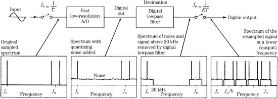
FIGURE 18.16 Diagram showing the theory of oversampling A/D conversion. (Adams, 1986)

Oversampling A/D converters are unusual in that the basic A/D elements of anti-alias filtering, sampling, and quantization are merged throughout the subsections of the converter. For example, anti-alias filtering occurs in both the input analog filter, and in the digital decimation filter. Although traditional A/D converters only perform quantization, oversampling A/D converters are complete signal acquisition interfaces.

A diagram illustrating oversampling A/D conversion is shown in Fig. 18.16. The input signal is first passed through an analog anti-aliasing filter, and the input signal is sampled at a very fast rate (for example, f _a= 64 × f_s) to extend the Nyquist frequency. The signal is applied to a coarse quantizer such as a sigma-delta converter, which adds (shaped) noise to the signal. The digital data is lowpass-filtered with a cutoff at the Nyquist frequency; this removes out-of-band noise components to prevent anti-aliasing. Finally, the signal is resampled at a lower rate (such as 48 kHz) for storage or processing using normal methods. A decimation lowpass filter bandlimits the wideband signal (to 20 kHz in Fig. 18.16) so that aliasing will not occur when the signal is subsampled at the lower output frequency. A sample-and-hold circuit is not needed because an input sample can be taken during every internal clock cycle. In successive approximation converters, the sampled analog value must be held for the number of clock cycles equal to the number of bits being converted.

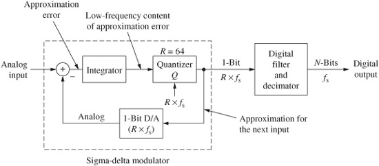
FIGURE 18.17 A first-order sigma-delta modulation circuit showing a one-bit D/A converter in the feedback loop.

Sigma-Delta A/D Modulator

A sigma-delta modulator can be used to create true one-bit coding from the lowpass-filtered input analog signal. A first-order sigma-delta A/D modulator is shown in Fig. 18.17. In this converter design, the sigma-delta modulator is followed by a digital filter and decimation stage. Because the input sampling rate is high, a simple one-pole RC anti-alias filter suffices. The modulator accepts a sampled analog signal, performs quantizing, and outputs a one-bit signal at a rate determined by the sampling clock. A low-resolution (one-bit quantizer) D/A converter operating at a high sampling rate is placed in a feedback loop. The input to the loop filter is the difference between the input signal and the quantized output converted back to an analog signal; this difference is theoretically equal to the quantization error. The average value of the D/A output (and the modulator output) must approach that of the input signal.

Because a coarse (one-bit A/D) quantizer is used, quantization error at sampling time is large. The coarse output signal is subsequently averaged by the decimation filter, interpolating over several samples (64 or so) to achieve a precise result. High resolution (manifested as dynamic range) is achieved through noise shaping. The integrator can be viewed in the frequency domain as an analog loop filter H(z). The noise-shaping characteristic in this sigma-delta modulator is the inverse of the transfer function of the filter. A filter with higher gain at low frequencies is thus desired to attenuate audio band noise. This transfer function is essentially a lowpass filter to the signal and a highpass filter to quantization noise; thus, the noise is shifted to a higher frequency. The higher the oversampling rate and order of noise shaping, the higher the resolution of the converter. For example, with an oversampling rate of 64, an ideal second-order modulator yields a signal-to-noise ratio of about 80 dB, equivalent to a 13-bit A/D resolution.

Instead of a one-bit code, converters might produce a multi-bit word of three or four bits using, for example, a sigma-delta modulator modified to contain a multi-bit quantizer. Several quantizer output bits are applied to an internal D/A converter and its analog output is subtracted from the analog input signal, thus producing a quantization error signal. This error signal is applied to the loop filter, and quantized to minimize error and thus yield an output that approximates the input. In this architecture, the dynamic range increases in proportion to the resolution of the quantizer; however, this must be balanced against operating speed. Dynamic range can also be increased by using higher-order filters. Because the output is proportional to the signal’s amplitude rather than slope, it is like a PCM converter. Unlike a traditional PCM converter, the noise floor rises with increasing frequency, at 6 dB/octave. Alternatively, a differential pulse code modulator differs from a delta modulator only in that the error signal is quantized to more than one bit. However, such an architecture is still slew-rate limited.

Numerous sigma-delta methods have been applied to A/D conversion, all using a high input sampling rate, and noise shaping. These methods include: single and dual integrator loops, cascaded first-order sigma-delta loops, and multi-bit quantizers with loop filters. The first two methods use true one-bit coders with inherent linearity. The third method uses several bits, and noise is reduced in proportion to the number of quantizer levels used. However, the converter’s linearity depends on the linearity of the quantizer. In any case, noise performance hinges on the oversampling rate and order of noise shaping used. Some converter architectures use several first- or second-order sigma-delta coders in combination to achieve higher order, stable noise shaping.

Given a second-order sigma-delta modulator, Charles Thompson has demonstrated that M-bit resolution requires an oversampling rate:

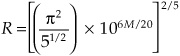
where R is the oversampling rate defined by:

where f_a = the oversampling frequency

f_s = the output sampling frequency

Thus, 16-bit resolution would require an oversampling rate of 150. A 100-kHz output sampling frequency would necessitate a filter sampling frequency of 15 MHz; this is difficult to achieve. If the order of noise shaping is raised to third-order, the required oversampling rate is described by:

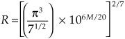
Thus, the required oversampling ratio is 48; this is well within practical design limits.

Depending on its order and design, a sigma-delta feedback loop generally performs the following operations: subtraction of output from input to find the approximation error, filtering to extract the low-frequency content of the approximation error, sigma-delta D/A conversion of the output code into a signal to subtract it from the input analog signal, and quantization to output an approximation for the next input sample. In practice, a third-order loop can be used to shape the noise toward higher frequencies, where it is removed by the subsequent decimation (undersampling) filter. As with any noise-shaping loop, the signal must be properly dithered to overcome idle tones and other artifacts. In some cases, a dither signal can be applied so that its fundamental and harmonics can be removed by the decimation filter.

Digital Filtering and Decimation

As Robert Adams has pointed out, oversampling converters provide high resolution not by decreasing the error between the analog input and the digital output, but by making the error occur more often. In this way the error spectrum moves beyond the audio passband and although the total noise power is high, the in-band noise power is low. The high bit rate is reduced to more manageable rates through decimation in which a discrete time signal is sampled at a rate lower than the original rate. Decimation provides both an averaging (lowpass) filter and rate reduction. It removes the high-frequency shaped noise, and provides an anti-aliasing function for the final sampling rate. Looked at in another way, decimation removes the redundant information created by oversampling.

Decimation can be described through a simple example. Sixteen one-bit values could be reduced through a 16:1 decimation to a single multi-bit value; for example, values 1,0,1,0,0,1,0,1,1,0,1,1,1,1,0,0 would be decimated to 9/16, or 0.5625. Because there is only one (multi-bit) output value for every 16 input values, the decimator has decreased the sampling rate by 16:1. As Sangil Park has shown, it is also important to note that decimation has increased resolution; in this example, the input signal is only one bit, but the decimation (averaging) process yields 4-bit resolution (2⁴ = 16) while reducing the sampling rate. Thus, oversampling followed by decimation demonstrates how speed can be exchanged for resolution. The meaning of the word decimation, incidentally, originally referred to a form of harsh discipline administered by the Roman army to punish cowardice. Soldiers selected for decimation were placed in groups of 10 and drew lots. The soldier on whom the lot fell was executed by his nine comrades, usually by clubbing or stoning.

The decimation process lowpass filters the signal and noise in the one-bit code, band-limiting the code prior to sample-rate reduction to remove alias components. Decimation also replaces the one-bit coding with 16-bit coding, for example, at a lower sampling rate. However, the computation rate of the filter is not trivial; output samples cannot be discarded (providing decimation) until the filtering computation is complete.

Ideally, the decimation filter would provide a sharp lowpass cutoff at half the output sampling frequency, thus upholding the Nyquist sampling theorem. However, as Robert Adams has shown, this is not always efficient. For example, an FIR filter would require many coefficients because of the high ratio of the input sampling rate to the output sampling rate. Still, when an FIR filter is used, filter outputs are only computed at the lower output sampling rate. An FIR filter is well-suited for decimation. If an IIR filter is used, the feedback loop dictates that an output value must be computed for every input. The decimation function cannot be combined as part of an IIR filter. A practical approach uses two or more stages of decimation, operating at intermediate sampling frequencies. For example, the first stage might use an FIR filter for decimation and a second stage might use an IIR filter for digital filtering. Alternatively, two-stage FIR filters, or two-stage IIR filters can be used, with both stages performing some decimation.

If the first stage resamples at an intermediate frequency f_i it would appear that all frequencies above f_i/2 must be rejected to prevent subsequent aliasing. However, only certain portions of the spectrum will alias in the audio band, thus the decimation filter need only attenuate those frequency bands. In particular, these alias bands can be identified:

f_alias = I × f₁ ± BW Hz

where I = any integer

f_i = the decimation filter’s intermediate resampling frequency

BW = the audio bandwidth (for example, 20 kHz)

For example, if f_i = 96 kHz, the bands of interest will lie at 96, 2 × 96, 3 × 96 kHz, and so on, each occupying a width of 40 kHz. The decimation filter can be designed so that its frequencies of maximum attenuation will coincide with these potentially aliasing frequency bands. A filter with pockets of attenuation, rather than attenuation across the entire stopband, is much easier to implement. As the sampling rate is decreased from one stage to the next, the pockets become proportionally wider and filter complexity increases, but intense computation is performed at the slower rate. In this way, each filter must only reject the signals that would be aliased by the immediate next decimation. Subsequent filters will reject signals that would alias with later decimation. A comb filter is an expedient choice because its design does not require a multiplier (all coefficients are unity).

However, as Sangil Park points out, comb filters cannot wholly remove out-of-band quantization noise so they are followed by additional filter stages of other design. These additional stages can also be needed to compensate for high-frequency drooping caused by the comb filter. A final filter, operating at the slowest sampling rate, could provide a true lowpass characteristic, and correct any frequency-response deviations. A comb filter of length R is an FIR filter with coefficients equal to unity; its transfer function is:

In other words, this expression shows a moving average. For example, if R = 4:

In recursive form, the transfer function can be written as:

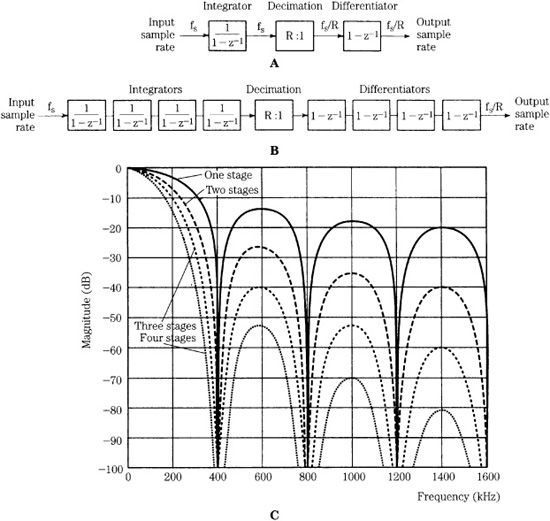
FIGURE 18.18 Comb filters can be used in decimation. A. Block diagram of a one-stage comb filter. B. Block diagram of a cascaded four-stage comb filter. C. Spectrum showing the response of one-, two-, three-, and four-stage cascaded comb filter sections. (Park, 1990b)

This can be expressed in terms of integration followed by differentiation:

This single-stage comb filter decimator can be easily realized, as shown in Fig. 18.18A. Not only is no storage required for the filter coefficients, but the burden of intermediate computations is decreased owing to the low sampling rate at the differentiator. In addition, the same topology can be used for higher orders of rate change. As noted, in practice, a single comb filter stage does not provide sufficient stopband attenuation to prevent aliasing, thus cascaded stages are often used, as shown in Fig. 18.18B. In this example, four sections are cascaded, requiring eight data registers and 4(R + 1) additions per input sample. As noted, the comb filter is designed for maximum attenuation at higher frequency components that would alias after rate decimation. Figure 18.18C shows the spectrum with one-, two-, three-, and four-stage cascaded comb filter sections.

In some decimator designs, the cascaded comb filter is followed by an FIR filter. The intermediate-rate output from the comb filter is further decimated and the FIR section provides sharp filtering when the sampling frequency is reduced to nominal values (for example, 48 kHz). The decimation factor is typically lower in the FIR section as compared to that in the comb filter section. However, the FIR filter must provide extreme stopband attenuation. In addition, the FIR section can provide compensation for audio band droop caused by the comb filter. FIR computation also provides a linear phase response.

Consider an example in which coding takes place at 64 × 48 kHz = 3.072 MHz. The decimation filter can have two stages. With a 64 × f_s Hz input bitstream, the first stage can generate a multi-bit output sample at a sampling frequency of 2 × f_s Hz. The second stage of the decimation filter can use a multi-bit multiplier with convolution performed at the output sampling frequency of f_s Hz. In all, the decimation filter provides a stopband from 20 kHz to the half-sampling frequency of 1.536 MHz. The analog filter at the system’s input is modest, perhaps first- or second-order, ensuring phase linearity in the audio band.

The use of one-bit coding as the intermediate phase of A/D conversion simplifies the filter design. For example, a new output sample is not required for every input bit. Because the decimation factor is 64 (in this example), an output is required only for every 64 input bits. In practice, the decimation filtering might be carried out in two stages. An FIR filter would commonly be used for downsampling, because its nonre-cursive operation would simplify computation to one sample every 1/f_s second. Following decimation, the result can be rounded to 16 bits, and output at a 48-kHz sampling frequency. Figure 18.19 summarizes the operation of a sigma-delta A/D converter in the frequency domain.

Digital audio equipment containing A/D (and D/A) converters must have a stable sampling clock that in turn is phase-locked to a distributed master clock. The individual clocks must have very low jitter levels to prevent generated sidebands from rising to audibility. For example, a 16-bit A/D converter might require jitter of less than 20 ps. Jitter is proportionally greater per period for a sigma-delta A/D converter than a ladder converter. Amplitude errors attributable to jitter increase as the input signal frequency increases. However, because the slew rate of the input signal is equal in either type of converter, the amplitude error resulting from sinusoidal jitter is also equal in both cases.

In the case of noise-induced jitter, added noise is distributed over the sigma-delta converter’s increased Nyquist frequency range and lowpass-filtered by the decimation circuit. Hence overall in-band jitter-induced noise is less than in some traditional converters. Thus analysis would show that oversampling sigma-delta A/D converters are generally no more sensitive to sinusoidal jitter than a traditional converter and are less susceptible to random noise clock jitter. However, actual performance depends on a converter’s specific design. For example, true one-bit converters are generally more susceptible to jitter than multi-bit converters. Timebase correction is discussed in Chap. 4.

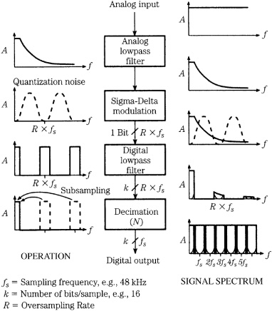
FIGURE 18.19 Summary of spectral characteristics of a one-bit A/D converter.

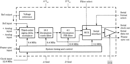
FIGURE 18.20 Internal block diagram of a DSP56ADC16 sigma-delta A/D converter. (Kloker et al., 1989)

Sigma-Delta A/D Converter Chip

The block diagram of a sigma-delta A/D converter chip is shown in Fig. 18.20. It is a linear 16-bit converter, using 64-times oversampling, providing output sampling frequencies up to 100 kHz, operating at up to 6.4 MHz. As with other sigma-delta A/D converters, the input signal is oversampled to extend the noise spectrum well beyond the audio band. Noise shaping reduces noise in the audio band, and lowpass-filtering removes out-of-band quantization noise. Finally, the signal is decimated to reduce the sample rate commensurate with the audio band and to increase resolution.

The converter is designed around four major blocks: third-order sigma-delta modulator and noise shaper, 16:1 decimation comb filter, 4:1 decimation FIR filter, and serial interface. The third-order noise shaper places an 18 dB/octave characteristic on the quantization noise. The analog front end to the converter consists of three differential, switched-capacitor, linear integrators. Filtering and decimation are performed in two steps to reduce the complexity of the digital filter. For example, to achieve the desired stopband attenuation and filter steepness, a single-stage FIR with over 2800 taps would be required. Use of a multirate decimation filter system also allows a dual mode application.

The output of the modulator is filtered by a fourth-order comb filter and decimated; the sampling rate is decreased by a factor of 16:1. A comb filter is used because it contains only adders and delay, without need for multiplication. The first stage comb filter accomplishes initial filtering as well as decimation of the input sampling rate by a factor of 16:1. Its z-domain transfer function can be expressed as:

The equivalent frequency domain transfer function is:

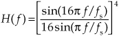
where f_s = the filter’s sampling frequency.

An FIR filter is used to decimate the signal by a 4:1 factor with a lowpass response. Overall, a 64:1 decimation ratio is achieved. In other words, 63 of every 64 output samples are discarded. A stopband attenuation of –96 dB is achieved. To compensate for the response (passband droop) of the fourth-order comb filter, the FIR uses an inverse equalization response to achieve an overall flat response. FIR images occur at multiples of the comb filter output sampling rate; these are also zeros in the fourth-order comb response. The FIR stopband attenuates the comb response, leaving a negligible alias component at the overlap of the two responses. In all, this digital filter section is the equivalent of a 30th-order analog Bessel filter. The output sampling frequency is 100 kHz, with 16-bit resolution and S/N ratio of 90 dB.

Because the cutoff frequencies of the comb and FIR filters are scaled by the input sampling rate, the converter can be used with any arbitrary sampling rate without changing component values. For further flexibility, this A/D converter chip is designed so the 16:1 comb filter can be connected directly to a serial output. This permits operation at faster speed (output sampling frequency of 400 kHz) at the expense of lower resolution (12 bit, and S/N of 72 dB). This is useful for ultrasonic applications and where lower resolution is tolerable. A general application for this chip using its full resolution is shown in Fig. 18.21; the A/D converter is connected to a DSP processor.

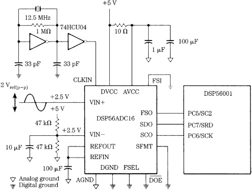
FIGURE 18.21 Application circuit showing an interconnection of a sigma-delta A/D converter (single-ended mode) and DSP processor.

Sigma-Delta D/A Converter Chip

A typical sigma-delta D/A converter comprises a digital interpolation filter, sigma-delta modulator, and switched-capacitor filter. The interpolation filter raises the input sampling frequency to the modulation rate. The modulator reduces the word length to one or a few bits and reduces in-band noise. The switched-capacitor elements filter outof-band noise and perform signal D/A reconstruction.

One example of a multi-bit sigma-delta D/A converter uses a second-order mismatch shaping function inside the feedback loop of a high-order modulator. This feature moves element mismatch noise to higher frequencies where it is removed along with other sigma-delta noise by lowpass-filtering. This feature is used in lieu of dynamic element matching (DEM) after the modulator. PCM or DSD data at sample rates up to 200 kHz is input via a serial port and passes through an interpolator and volume control, as shown in Fig. 18.22. DSD data is volume-adjusted and upsampled by a factor of 2. Data is applied to a sixth-order sigma-delta modulator with integrated second-order mismatch noise shaping. To ensure stability, a fallback second-order sigma-delta modulator can be used. The mismatch noise shaping is not changed when in the fallback mode. When processing SACD data, the modulator also uses a fifth-order Butter-worth lowpass filter with a corner frequency of 50 kHz.

The mismatch shaper effectively provides 16 second-order loops with the first and second integrals using 16 elements. The main quantizer outputs the number of elements that the mismatch shaper should turn on. The shaper can override this value to optimize noise shaping. The number of elements actually turned on is used in the main feedback loop. Even with an element mismatch of 5%, a signal-to-noise ratio of 129 dB is still achieved. Mismatch shaping can continue for full-scale signals. Some DEM designs can introduce a data-dependent noise floor when given a high-level signal and all elements are turned on. The analog output stage comprises a 16-element switched-capacitor D/A converter operating at 6 MHz.

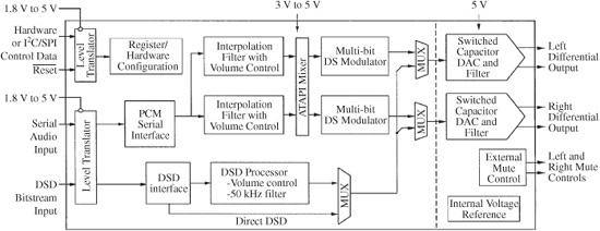
FIGURE 18.22 System architecture of a multi-bit sigma-delta D/A converter with mismatch shaping in the feedback loop. (Deuwer et al., 2003)

In this design, the noise shaper is inside the main loop; a balance is struck between quantization error and element mismatch error, determined by the number of elements the mismatch shaper turns on. When the quantizer’s output is not followed, quantization error increases. The noise contribution from the main loop quantization error, assuming no mismatch, is set equal to the noise from mismatch shaping error, assuming worst case element mismatch.

As with other multi-bit converters, this converter has relatively low quantization noise, low sensitivity to clock jitter, and fewer idle tones compared to many one-bit converters. This design outputs a bitstream compatible with SACD without a decimation filter following the multi-bit conversion. A dynamic range of 120 dB (A-weighted) and distortion level of −105 dB THD+N can be achieved. Converters such as this are used for CD/SACD/DVD/Blu-ray playback.

Sigma-Delta A/D–D/A Converter Chip

Because of the high degree of integration permitted by sigma-delta conversion methods, it is possible to place a linear, 16-bit sigma-delta analog-to-digital and digital-to-analog converter on a single chip. One such chip permits input-output sampling frequencies up to 50 kHz with 16-bit resolution, and frequencies of 100 kHz with 12-bit resolution. Third-order noise shaping is used on the A/D side, and fourth-order noise shaping is used on the D/A side. The A/D section uses 64-times oversampling and 64-times decimation. A digital compensation circuit is used to equalize the response to within ±0.025-dB ripple in the passband, with phase linearity.

The D/A section uses two digital anti-imaging interpolation filters, along with an FIR compensation filter for flat passband response. The D/A section provides the output signal. An analog sixth-order Bessel lowpass filter is provided on-chip, as is a temperature-compensated voltage reference for stable coding and clocking. This reference can operate in a master–slave configuration to ensure gain matching and tracking between multiple devices. Likewise, sampling coherency can be preserved between multiple converter chips to ensure interchannel phase accuracy. Digital data can be shifted into and out of the converters with either MSB or LSB first. An SSI bus can be implemented in several different modes.

The DSP56ADA16 provides a dynamic range of 96 dB and signal-to-noise ratio of 90 dB. As with all sigma-delta converters, this converter pair is based on digital filtering techniques, thus approximately 90% of the chip is given to digital circuitry. This promotes compatibility, reliability, increased functionality, and reduced chip cost. Two of these chips form a complete conversion circuit for a stereo signal, and together with a DSP56xxx chip form a complete digital signal processing system.

Noise Shaping of Nonoversampling Quantization Error

As noted, noise shaping is prerequisite in any sigma-delta system to preserve dynamic range when a signal is represented with a reduced number of bits. For example, the noise-shaping characteristic of sigma-delta converters allows one-bit quantization. However, noise shaping can be applied in a variety of ways. For example, a noise-shaping feedback loop can be placed around a quantizer, as shown in Fig. 18.23. This noise-shaping loop uses the known characteristics of the error generated by the word length reduction (requantization) to alter the spectrum of the requantization noise error.

Recursion places the error information back into the signal, much like negative feedback is used to reduce distortion in analog amplifiers. The quantizer’s output error is fed back through a filter and subtracted from the quantizer’s input. Because only the difference between the input and output of the quantizer is fed back, the input signal is not affected. The configuration alters the frequency response of the error signal, but not that of the audio signal. It has the effect of passing the noise through the filter, not the signal.

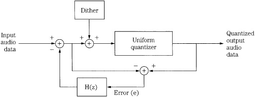
FIGURE 18.23 A requantization topology showing dithering and noise shaping. This processing reduces quantization distortion artifacts and can be used to reduce the noise floor in perceptually critical frequency regions.

However, with proper dither, the error is white, and the H(z) filter in the feedback loop spectrally shapes the output error by 1 – H(z). That is, the output error e becomes: [1 – H(z)]e. The noise is shaped by the inverse of the loop transfer function; when a lowpass filter is placed in the loop, the noise spectrum rises with frequency. A filter with high gain at low frequencies yields improved baseband attenuation of noise. Higher-order functions perform a higher-order difference operation on quantizer error, with greater attenuation of baseband noise. The frequency response of the requantization noise can be creatively manipulated by the filter in the feedback loop. For example, the filter’s parameters could be dynamically adapted so that the error noise is always optimally masked by the audio signal. The feedback loop must incorporate at least a one-sample z⁻¹ delay; the error cannot be processed until after it has been created by quantization. Theory also dictates that 1 – H(z) must be minimum phase (all poles and zeros within the z-plane unit circle) to preserve the capacity of the channel.

Referring again to Fig. 18.23, John Vanderkooy and Stanley Lipshitz have pointed out that H(z) represents a loop error that is subtracted from the input at each next sample. This corrects for any such errors on average and gives a highpass shape to both quantization and dither signals present inside the loop. A digital dither signal applied as shown (inside the shaping loop) is identical to a highpass-filtered dither signal applied at a point outside the loop prior to the quantizer. Figure 18.24A shows the spectrum of the quantized output of an undithered noise shaper when a 937.5-Hz signal of 1-LSB peak amplitude (approximately –90.3 dBFS) is passed though an undithered requantizer. The spectrum shows many correlated errors with this low-level input signal.

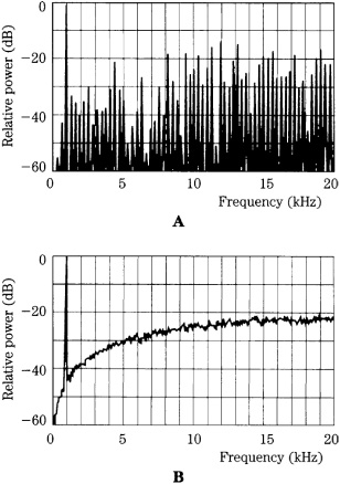
FIGURE 18.24 Dither profoundly affects the spectrum of the signal output from a noise-shaping circuit. A. Spectrum of a signal with an undithered noise shaper. B. Spectrum of the signal with a triangular pdf-dithered noise shaper. (Vanderkooy and Lipshitz, 1989)

When triangular pdf digital dither is applied, a highly uncorrelated spectrum results, as shown in Fig. 18.24B. The quantizer and the dither signal noise are both shaped by the loop. A rectangular pdf dither signal could be applied, but could result in noise modulation and limit cycle oscillation. The latter is a repeating output sequence that will produce spectral lines that can yield audible distortion. Alternatively, a high-pass triangular pdf dither could be applied; requantization noise is shaped as before, but the higher frequency dither signal is shaped to even higher frequencies. However, correlation can result in higher overall noise. In this example, triangular pdf dither with a white spectrum appears to yield the best results.

Psychoacoustically Optimized Noise Shaping

The goal of noise-shaping systems is to dither the audio signal, then shape quantization noise to yield a less audible noise floor. These systems consider the fact that total noise power does not fully describe audibility of noise; perceived loudness also depends on spectral characteristics. Oversampling noise shapers reduce audio-band quantization noise and increase noise beyond the audio band, where it is inaudible. Nonoversampling noise shapers only redistribute noise energy within the audio band itself. For example, the difference in quantization noise between a 20-bit input signal and a 16-bit output signal can be reshaped to minimize its audibility. In particular, psychoacoustically optimized noise-shaping systems use a feedback filter designed to shape the noise according to an equal-loudness contour or other perceptual weighting function. In addition, such systems can use masking properties to conceal requantization noise.

Sixteen-bit master recordings are not adequate for subsequent music distribution on 16-bit media; for example, for replication of 16-bit CDs. When using a digital console or hard-disk recorder to add equalization, change levels, or perform other digital signal processing, error accumulates in the 16th bit due to computation. It is desirable to use a longer word length, such as 20 bits, that allows processing prior to 16-bit storage. Furthermore, with proper transfer, much information contained in the four LSBs can be conveyed in the upper 16 bits. However, the problem of transferring 20 bits to 16 bits is not trivial. Simple truncation of the four least-significant bits greatly increases distortion. If the 16th bit is rounded, the improvement is only modest.

It is thus important to redither the signal during the requantization that occurs in the transfer. This provides the same benefits as dithering during the original recording. If the most significant bit has not been exercised in the recording, it is possible to bit-shift the entire program upward, thus preserving more of the dynamic range. This is accomplished with a simple gain change in the digital domain. It can be argued that in some cases, for example, when transferring from an analog master tape, a 20-bit interface and noise shaping are not needed because the tape’s noise floor makes it self-dithering. However, even then it is important to preserve the analog noise floor which contains useful audio information.

Nonoversampling noise-shaping systems are often used when converting a professional master recording to a consumer format such as a CD. With linear conversion and dither, a 16-bit recording can provide a distortion floor below –110 dBFS. Noise shaping cannot decrease total unweighted noise, but given a 20-bit master recording, subjective performance can be improved by decreasing noise in the critical 1-kHz to 5-kHz region, at the expense of increasing noise in the non-critical 15-kHz region, and increasing total unweighted noise power as well. Because noise shaping removes requantization noise in the most critical region, this noise cannot mask audible details, thus improving subjective resolution. However, the benefit is realized only when output D/A converters exhibit sufficient low-level linearity, and high S/N ratio is available. Indeed, any subsequent requantization must preserve the most critical noise floor improvements, and not introduce other noise that would negate the advantage of a shaped noise floor. For example, 19-bit resolution in D/A converters may be required to fully preserve noise-shaping improvements in a 16-bit recording.

When reducing word length, the audio signal must be redithered for a level appropriate for the receiving medium, for example, 16 bits for CD storage; white triangular pdf dither can be used. A nonoversampling noise-shaping loop redistributes the spectrum of the requantization noise. As noted earlier in this chapter, sigma-delta noise shapers used in highly oversampled converters yield a contour with a gradually increasing spectral characteristic. This characteristic will not specifically reduce noise in the 1-kHz to 5-kHz region. To take advantage of psychoacoustics, higher-order shapers are used in nonoversampling shapers to form more complicated weighting functions. In this way, the perceptually weighted output noise power is minimized. A digital filter H(z) in a feedback loop (see Fig. 18.23) accomplishes this, in which the filter coefficients determine a response so that the output noise is weighted by 1 – H(z), the inverse of the desired psychoacoustic weighting function. The resulting weighted spectrum ideally produces a noise floor that is equally audible at all frequencies.

As Robert Wannamaker suggests, a suitable filter design begins with the selection of a weighting function. This design curve is inverted, and normalized to yield a zero average spectral power density that represents the squared magnitude of the frequency response of the minimum-phase noise shaper. The desired response is specified, and an inverse Fourier transform is applied to produce an impulse response. The response is windowed to produce a number of filter coefficients corresponding to 1 – H(z), then H(z) is derived from this, yielding an FIR filter.

Theory shows that as very high-order filters H(z) are used to approximate the optimal filter weighting function, the unweighted noise power increases, tending toward infinity with an infinite filter order. For example, although an optimal approximation might yield a 27-dB decrease in audible weighted noise (using a particular weighting curve that reflects the ear’s high-frequency roll-off), other weighting functions must be devised, with more modest performance. For example, using a nine-coefficient FIR shaping filter, perceived noise can be decreased by 17 dB compared to unshaped requantization noise. Total unweighted noise power is increased by a reasonable 18 dB compared to an unshaped spectrum. In other words, the output is subjectively as quiet as an unshaped truncated signal with an additional three bits. In this way, audio data with resolution of 19 bits can be successfully transferred to a 16-bit CD. Similar techniques, of course, are applicable to DVD and Blu-ray authoring, when 16-, 20-, or 24-bit words may be used.

Methods that decrease audible noise while increasing total noise (at higher inaudible frequencies) perform a delicate balance. For example, a very high total noise power might damage tweeters, and some listeners suggest that aggressively boosted high-frequency noise produces artifacts, or perhaps masks otherwise audible information. In practice, depending on the design, the weighting function often approximates a proprietary contour. For example, Fig. 18.25 shows a proprietary noise-shaping contour, plotted with linear frequency for clarity. In some cases, this curve is fixed; in other cases, the curve is adaptively varied according to signal conditions. Similarly, in some designs, an adaptive dither signal is correlated to the audio signal so the audio signal masks the added dither noise. For example, the audio signal can be spectrally analyzed so that dither frequencies slightly higher in frequency can be generated.

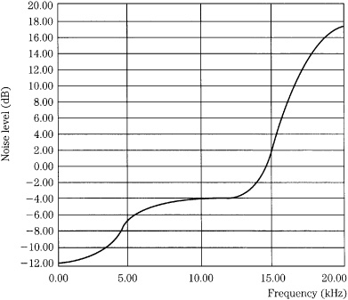
FIGURE 18.25 An equal-loudness noise-shaping curve. This frequency response plot uses a linear scale to better illustrate the high-frequency contour. (Akune et al., 1992)

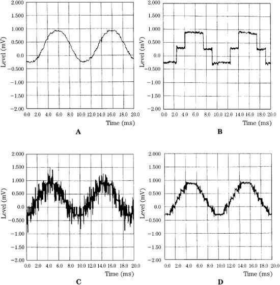
FIGURE 18.26 An example of noise shaping showing a 1-kHz sine wave with −90-dBFS amplitude. Measurements are made with a 16-kHz lowpass filter. A. Original 20-bit recording. B. Truncated 16-bit signal. C. Dithered 16-bit signal. D. Noise shaping preserves information in the lower 4 bits.

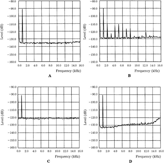
FIGURE 18.27 An example of noise shaping showing the spectrum of a 1 kHz, –90-dBFS sine wave (from Fig. 18.26). A. Original 20-bit recording. B. Truncated 16-bit signal. C. Dithered 16-bit signal. D. Noise shaping reduces low- and mid-frequency noise, with an increase at higher frequencies.

Figure 18.26 shows a 1-kHz sine wave with –90-dBFS amplitude. Measurements are made with a 16-kHz lowpass filter, to approximate the ear’s averaging response. A 20-bit recording is quite accurate; when truncated to 16 bits, quantization is clearly evident; when dithered (±1 LSB triangular pdf) to 16 bits, quantization noise is alleviated, but noise is increased; when noise shaping is applied, the noise in this lowpass-filtered measurement is reduced. This 16-bit representation is quite similar to the original 20-bit representation. Figure 18.27 shows the spectrum of the same –90-dBFS sine wave, with the four representations. The 20-bit recording has low error and noise; truncation creates severe quantization error; dithering removes the error but increases noise; noise shaping reduces low- and mid-frequency noise, with an increase at higher frequencies.

In one implementation of a psychoacoustic noise shaper, adaptive error-feedback filters are used to optimize the requantization noise spectrum according to equal-loudness contours as well as masking analysis of the input signal. An algorithm analyzes the signal’s masking properties to calculate simultaneous masking curves. These are adaptively combined with equal-loudness curves to calculate the noise-shaping filter’s coefficients, to yield the desired contour. This balance is dynamically and continuously varied according to the power of the input signal. For example, when power is low, masking is minimal, so the equal-loudness contour is used. Conversely, when power is high, masking is prevalent so the masking contour is more prominently used.

The input signal is converted into critical bands, convolved with critical-band masking curves, and converted to linear frequency to form the masking contour and hence the noise-shaping contour. In other words, masking analysis follows the same processing steps as used in perceptual coding.

Buried Data Technique

With proper dithering and noise shaping, dynamic range can be improved. However, processing can also be applied to use this dynamic range for purposes other than conventional audio headroom. Michael Gerzon and Peter Craven have demonstrated how data can be “buried” in a bitstream. The data is coded with psychoacoustic considerations so the data is inaudible under the masking curve of the audio program; the added data signal is randomized to act as shaped noise. For example, the method could be used to place new information on conventional audio CDs, without significantly degrading the quality of the audio program. In particular, this coding technique replaces several of the least-significant bits of the 16-bit format with independent data. Clearly, if unrelated data simply displaced audio data, and the disc was played in a conventional CD player, the result would be unlistenable. For example, nonstandard data in the four least-significant bits would add about 27 dB of noise to the music, as well as distortion caused by truncating the 16-bit audio signal. The buried data method makes buried data discs compatible with conventional CD players. However, a separate decoder is needed to utilize the buried data.

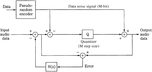
FIGURE 18.28 A buried data channel encoder converts added data to a pseudo-random noise signal, which is used as a dither signal. This is subtracted from the audio signal prior to quantization and added to the signal after quantization. Noise shaping is performed around the quantizer. (Gerzon and Craven, 1995)

An example of the subtractively dithered, noise-shaped quantizer used to encode buried data is shown in Fig. 18.28. For example, a 16-bit signal is quantized with an M-bit step size (rounding the signal to the nearest integer multiple of M) to yield a (16–M)-bit signal. The buried data is coded to be pseudo-random, to make it noise-like with a uniform probability density function. This signal is used as subtractive M-bit dither to remove the artifacts caused by quantization. Specifically, the data dither is subtracted prior to quantization, and then added after quantization, replacing the M least-significant bits of the signal. The quantizing error signal is statistically independent of the input audio signal. To reduce the audibility of the resulting increase in the noise floor, a noise-shaping filter is applied in a loop around the quantizer so that the shaped noise is subtracted from the input signal. The transfer function H(z) is selected so that 1 – H(z) yields a noise floor that ideally lies below the threshold of audibility. Through noise shaping, the noise created by four bits of buried data per channel (conveying 352.8 kbps with stereo channels) can be reduced to yield an overall S/N ratio of about 91 dB, a level that is similar to conventional CDs. Two bits of buried data provide a buried channel rate of 176.4 kbps, while maintaining an S/N ratio of 103 dB.

The average bit rate of the buried data could be increased by variably “stealing” bits from the original program only when their absence will be psychoacoustically masked by the music signal. By using an adaptive noise-shaping filter and a variable quantizer step size, the noise-shaping characteristic is varied according to the analyzed masking properties of the signal and the noise can be maintained below the masking threshold. The overall buried data rate could exceed 500 kbps, with 800 kbps possible during loud passages, depending on the music program. Combining methods, for example, buried data might consist of two 2-bit fixed channels, and a variable rate channel; side information would indicate the variable data rate. A buried data CD could be played in a regular CD player; the fidelity of music with limited dynamic range might not be affected at all.

More significantly, a CD player with appropriate decoding (or a player outputting buried data to an external decoder) could play the original music signal, and process buried data as well. The possibilities for buried data are numerous; many audio improvements can be more useful than the lost dynamic range. For example, buried 4-bit data could be used to convey multiple (5.1 channel) audio channels for surround-sound playback; the main left/rights channels are conventionally coded, the buried data carries four additional channels. A hybrid disc would compatibly deliver stereo reproduction with a conventional CD player, and surround sound with a 5.1-channel CD player.

Alternatively, one or two bits of buried data could carry dynamic range compression or expansion information. Depending on the playback circumstances, the dynamic range of the music could be adjusted for the most desirable characteristics. Because the range algorithms are calculated prior to playback, they are much more effective than conventional real-time dynamic processing. Buried data could convey additional high-frequency information above the Nyquist frequency, and provide a gentle bandlimiting roll-off rate. Any of these applications could be combined, within the limits of the buried data’s rate. For example, two ambience channels and dynamic range control data could be delivered simultaneously. Techniques such as these demonstrate the utility of noise shaping and further underscore the power of digital signal processing in digital audio applications.