
CHAPTER
SIXTY
PRICING FUTURES AND PORTFOLIO APPLICATIONS
FRANK J. FABOZZI, PH.D., CFA, CPA
Professor of Finance
EDHEC Business School
MARK PITTS, PH.D.
BRUCE M. COLLINS, PH.D.
Professor of Finance
Western Connecticut State University
One of the primary concerns most traders and investors have when taking a position in futures contracts is whether the futures price at which they transact will be a fair price. Buyers are concerned that the price may be too high and that they will be picked off by more experienced futures traders waiting to profit from the mistakes of the uninitiated. Sellers worry that the price is artificially low and that savvy traders may have manipulated the markets so that they can buy at bargain-basement prices. Furthermore, prospective participants frequently find no rational explanation for the sometimes violent ups and downs that occur in the futures markets. Theories about efficient markets give little comfort to anyone who knows of or has experienced the sudden losses that can occur in the highly leveraged futures markets.
Fortunately, the futures markets are not as irrational as they may at first seem; if they were, they would not be so successful. The interest-rate futures markets are not perfectly efficient markets, but they probably come about as close as any market. Furthermore, there are very clear reasons why futures prices are what they are, and there are methods by which traders, investors, and borrowers will quickly eliminate any discrepancy between futures prices and their fair levels.
In this chapter we will explain how the fair or theoretical value of a futures contract is determined. We then explain several portfolio applications of interest-rate futures.
PRICING OF FUTURES CONTRACTS
There are several different ways to price futures contracts. Fortunately, all lead to the same fair price for a given contract. Each approach relies on the law of one price. This law states that a given financial asset (or liability) must have the same price regardless of the means by which one goes about creating that asset (or liability). In this section we will demonstrate one way in which futures contracts can be combined with cash market instruments to create cash-flows that are identical to other cash securities.1 The law of one price implies that the synthetically created cash securities must have the same price as the actual cash securities. Similarly, cash instruments can be combined to create cash-flows that are identical to futures contracts. By the law of one price, the futures contract must have the same price as the synthetic futures created from cash instruments.
Illustration of the Basic Principles
To understand how futures contracts should be priced, consider the following example. Suppose that a 20-year 100 par value bond with a coupon rate of 12% is selling at par. Also suppose that this bond is the deliverable for a futures contract that settles in three months. If the current three-month interest rate at which funds can be loaned or borrowed is 8% per year, what should be the price of this futures contract?
Suppose the price of the futures contract is 107. Consider the following strategy:
Sell the futures contract at 107.
Purchase the bond for 100.
Borrow 100 for three months at 8% per year.
The borrowed funds are used to purchase the bond, resulting in no initial cash outlay for this strategy. Three months from now, the bond must be delivered to settle the futures contract and the loan must be repaid. These trades will produce the following cash-flows:

This strategy will guarantee a profit of 8. Moreover, the profit is generated with no initial outlay because the funds used to purchase the bond are borrowed. The profit will be realized regardless of the futures price at the settlement date. Obviously, in a well-functioning market, arbitrageurs would buy the bond and sell the futures, forcing the futures price down and bidding up the bond price so as to eliminate this profit. This strategy of purchasing a bond with borrowed funds and simultaneously selling a futures contract to generate an arbitrage profit is called a cash and carry trade.
In contrast, suppose that the futures price is 92 instead of 107. Consider the following strategy:
Buy the futures contract at 92.
Sell (short) the bond for 100.
Invest (lend) 100 for three months at 8% per year.
Once again, there is no initial cash outlay. Three months from now a bond will be purchased to settle the long position in the futures contract. That bond will then be used to cover the short position (i.e., to cover the short sale in the cash market). The outcome in three months would be as follows:

The 7 profit is a pure arbitrage profit. It requires no initial cash outlay and will be realized regardless of the futures price at the settlement date. Because this strategy involves initially selling the underlying bond, it is called a reverse cash and carry trade.
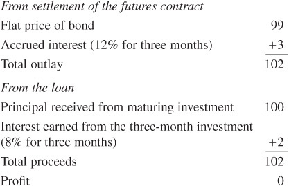
There is a futures price, however, that will eliminate the arbitrage profit. There will be no arbitrage if the futures price is 99. Let’s look at what would happen if the two previous strategies were followed and the futures price were 99. First, consider following cash and carry trade:
Sell the futures contract at 99.
Purchase the bond for 100.
Borrow 100 for three months at 8% per year.
In three months, the outcome would be as follows:

There is no arbitrage profit.
Next, consider the following reverse cash and carry trade:
Buy the futures contract at 99.
Sell (short) the bond for 100.
Invest (lend) 100 for three months at 8% per year.
The outcome in three months would be as follows:
Thus neither strategy results in a profit. The futures price of 99 is the equilibrium price because any higher or lower futures price will permit arbitrage profits.
Theoretical Futures Price Based on Arbitrage Model
Considering the arbitrage arguments just presented, the equilibrium futures price can be determined on the basis of the following information:
• The price of the bond in the cash market.
• The coupon rate on the bond. In our example, the coupon rate was 12% per annum.
• The interest rate for borrowing and lending until the settlement date. The borrowing and lending rate is referred to as the financing rate. In our example, the financing rate was 8% per annum.
We will let
r = financing rate
c = current yield, or coupon rate divided by the cash market price
P = cash market price
F = futures price
t = time, in years, to the futures delivery date
and then consider the following cash and carry trade that is initiated on a coupon date:
Sell the futures contract at F.
Purchase the bond for P.
Borrow P until the settlement date at r.
The outcome at the settlement date is as follows:

The profit will equal
Profit = total proceeds – total outlay
Profit = F + ctP - (P + rtP)
In equilibrium, the theoretical futures price occurs where the profit from this strategy is zero. Thus, to have equilibrium, the following must hold:
0 = F + ctP – (P + rtP)
Solving for the theoretical futures price, we have
![]()
Alternatively, consider the following reverse cash and carry trade:
Buy the futures contract at F.
Sell (short) the bond for P.
Invest (lend) P at r until the settlement date.
The outcome at the settlement date would be as follows:

The profit will equal
Profit = total proceeds – total outlay
Profit = P + rtP – (F + ctP)
Setting the profit equal to zero so that there will be no arbitrage profit and solving for the futures price, we obtain the same equation for the futures price as Eq. (60–1).
Let’s apply Eq. (60–1) to our previous example in which
r = 0.08
c = 0.12
P = 100
t = 0.25
Then the theoretical futures price is
F = 100 + 100 × 0.25(0.08 – 0.12)
= 100 – 1 = 99
This agrees with the equilibrium futures price we derived earlier.
The theoretical futures price may be at a premium to the cash market price (higher than the cash market price) or at a discount from the cash market price (lower than the cash market price), depending on the value of (r – c). The term r – c is called the net financing cost because it adjusts the financing rate for the coupon interest earned. The net financing cost is more commonly called the cost of carry, or simply carry. Positive carry means that the current yield earned is greater than the financing cost; negative carry means that the financing cost exceeds the current yield. The relationships can be expressed as follows:

In the case of interest-rate futures, carry (the relationship between the short-term financing rate and the current yield on the bond) depends on the shape of the yield-curve. When the yield-curve is upward-sloping, the short-term financing rate will generally be less than the current yield on the bond, resulting in positive carry. The futures price will then sell at a discount to the cash price for the bond. The opposite will hold true when the yield-curve is inverted.
A Closer Look at the Theoretical Futures Price
To derive the theoretical futures price using the arbitrage argument, we made several assumptions. We will now discuss the implications of these assumptions.
Interim Cash-Flows. No interim cash-flows owing to variation margin or coupon interest payments were assumed in the model. However, we know that interim cash-flows can occur for both of these reasons. Because we assumed no variation margin, the price derived is technically the theoretical price for a forward contract (which is not marked to market at the end of each trading day). If interest rates rise, the short position in futures will receive margin as the futures price decreases; the margin can then be reinvested at a higher interest rate. In contrast, if interest rates fall, there will be variation margin that must be financed by the short position; however, because interest rates have declined, the financing can be done at a lower cost. Thus, whichever way rates move, those who are short futures gain relative to those who are short forward contracts that are not marked to market. Conversely, those who are long futures lose relative to those who are long forward contracts that are not marked to market. These facts account for the difference between futures and forward prices.
Incorporating interim coupon payments into the pricing model is not difficult. However, the value of the coupon payments at the settlement date will depend on the interest rate at which they can be reinvested. The shorter the maturity of the futures contract and the lower the coupon rate, the less important the reinvestment income is in determining the theoretical futures price.
The Short-Term Interest Rate (Financing Rate). In deriving the theoretical futures price, it is assumed that the borrowing and lending rates are equal. Typically, however, the borrowing rate is greater than the lending rate.
We will let
rB = borrowing rate
rL = lending rate
Consider the following strategy:
Sell the futures contract at F.
Purchase the bond for P.
Borrow P until the settlement date at rB.
The futures price that would produce no arbitrage profit is
![]()
Now consider the following strategy:
Buy the futures contract at F.
Sell (short) the bond for P.
Invest (lend) P at rL until the settlement date.
The futures price that would produce no profit is
![]()
Equations (60–2) and (60–3) together provide boundaries for the theoretical futures price. Equation (60–2) provides the upper boundary, and Eq. (60–3) the lower boundary. For example, assume that the borrowing rate is 8% per year, or 2% for three months, and the lending rate is 6% per year, or 1.5% for three months. Then, using Eq. (60–2) and the previous example, the upper boundary is
F(upper boundary) = $100 + $100(0.02 – 0.03)
= $99
The lower boundary using Eq. (60–3) is
F(lower boundary) = 100 + $100(0.015 – 0.03)
= $98.50
In calculating these boundaries, we assumed no transaction costs were involved in taking the position. In actuality, the transaction costs of entering into and closing the cash position as well as the round-trip transaction costs for the futures contract, must be considered and do affect the boundaries for the futures contract.
Deliverable Bond and Settlement Date Unknown. In our example, we assumed that only one bond is deliverable and that the settlement date occurs three months from now. As explained in Chapter 59, futures contracts on Treasury bonds and Treasury notes are designed to allow the short position the choice of delivering one of a number of deliverable issues. Also, the delivery date is not known.
Because there may be more than one deliverable, market participants track the price of each deliverable bond and determine which is the cheapest to deliver. The futures price will then trade in relation to the bond that is cheapest to deliver.
The cheapest to deliver is the bond or note that will result in the smallest loss or the greatest gain if delivered by the short futures position.2
In addition to the reasons we have already discussed, there are several reasons why the actual futures price will diverge from the theoretical futures price based on the arbitrage model. First, there is the risk that although an issue may be the cheapest to deliver at the time a position in the futures contract is taken, it may not be the cheapest to deliver after that time. Thus, there will be a divergence between the theoretical futures price and the actual futures price. A second reason for this divergence is the other delivery options granted the short position. Finally, there are biases in the CME conversion factors.
Deliverable Is a Basket of Securities. The municipal index futures contract is a cash settlement contract based on a basket of securities. The difficulty in arbitraging this futures contract is that it is too expensive to buy or sell every bond included in the index. Instead, a portfolio containing a smaller number of bonds may be constructed to track the index. The arbitrage, however, is no longer risk-free because there is the risk that the portfolio will not track the index exactly. This is referred to as tracking-error risk. Another problem in constructing the portfolio so that the arbitrage can be performed is that the composition of the index is revised periodically. Therefore, anyone using this arbitrage trade must constantly monitor the index and periodically rebalance the constructed portfolio.
APPLICATIONS TO PORTFOLIO MANAGEMENT
This section describes various ways in which a money manager can use interest-rate futures contracts.
Interest-Rate Risk Control
Interest-rate risk control is probably the most common use of interest rate futures. This is accomplished by altering the portfolio’s duration. Money managers who have strong expectations about the direction of interest rates will adjust the duration of their portfolio to capitalize on their expectations. Specifically, if they expect interest rates to increase, they will shorten the duration of the portfolio; if they expect interest rates to decrease, they will lengthen the duration of the portfolio. Also, anyone using structured portfolio strategies must periodically adjust the portfolio duration to match the duration of some benchmark.
Although money managers can alter the duration of their portfolios with cash market instruments, a quick and less expensive means for doing so (especially on a temporary basis) is to use futures contracts. By buying futures contracts on Treasury bonds or notes, they can increase the duration of the portfolio. Conversely, they can shorten the duration of the portfolio by selling futures contracts on Treasury bonds or notes.
Hedging
Hedging is a special case of interest-rate risk control whereby the manager seeks to obtain a duration of zero.3 Hedging with futures involves taking a futures position as a temporary substitute for transactions to be made in the cash market at a later date. If cash and futures prices move together, any loss realized by the hedger from one position (whether cash or futures) will be offset by a profit on the other position. When the net profit or loss from the positions are exactly as anticipated, the hedge is referred to as a perfect hedge.
In practice, hedging is not that simple. The amount of net profit will not necessarily be as anticipated. The outcome of a hedge will depend on the relationship between the cash price and the futures price when a hedge is placed and when it is lifted. The difference between the cash price and the futures price is called the basis. The risk that the basis will change in an unpredictable way is called basis risk.
In most hedging applications, the bond to be hedged is not identical to the bond underlying the futures contract. This kind of hedging is referred to as cross-hedging. There may be substantial basis risk in cross-hedging. An unhedged position is exposed to price risk, the risk that the cash market price will move adversely. A hedged position substitutes basis risk for price risk.
A short (or sell) hedge is used to protect against a decline in the cash price of a fixed income security. To execute a short hedge, futures contracts are sold. By establishing a short hedge, the hedger has fixed the future cash price and transferred the price risk of ownership to the buyer of the futures contract. As an example of why a short hedge would be executed, suppose that a pension fund manager knows that bonds must be liquidated in 40 days to make a $5 million payment to the beneficiaries of the pension fund. If interest rates rise during the 40-day period, more bonds will have to be liquidated to realize $5 million. To guard against this possibility, the manager would sell bonds in the futures market to lock in a selling price.
A long (or buy) hedge is undertaken to protect against an increase in the cash price of a fixed income security. In a long hedge, the hedger buys a futures contract to lock in a purchase price. A pension fund manager may use a long hedge when substantial cash contributions are expected and the manager is concerned that interest rates will fall. Also, a money manager who knows that bonds are maturing in the near future and expects that interest rates will fall can employ a long hedge to lock in a rate.
Asset Allocation
A pension sponsor may wish to alter the composition of the pension fund’s assets between stocks and bonds. An efficient means of changing asset allocation is to use financial futures contracts: interest-rate futures and stock index futures.
Creating Synthetic Securities for Yield Enhancement
A cash market security can be synthetically created by using a position in the futures contract together with the deliverable instrument. The yield on the synthetic security should be the same as the yield on the cash market security. If there is a difference between the two yields, it can be exploited so as to enhance the yield on the portfolio.
To see how, consider an investor who owns a 20-year Treasury bond and sells Treasury futures that call for the delivery of that particular bond three months from now. The maturity of the Treasury bond is 20 years, but the investor has effectively shortened the maturity of the bond to three months.
Consequently, the long position in the 20-year bond and the short futures position are equivalent to a long position in a three-month riskless security. The position is riskless because the investor is locking in the price that he or she will receive three months from now—the futures price. By being long the bond and short the futures, the investor has synthetically created a three-month Treasury bill. The return the investor should expect to earn from this synthetic position should be the yield on a three-month Treasury bill. If the yield on the synthetic three-month Treasury bill is greater than the yield on the cash market Treasury bill, the investor can realize an enhanced yield by creating the synthetic short-term security. The fundamental relationship for creating synthetic securities is as follows:
![]()
where
CBP = cash bond position
BFP = bond futures position
RSP = riskless short-term security position
A negative sign before a position means a short position. In terms of our previous example, CBP is the long cash bond position, the negative sign before BFP refers to the short futures position, and RSP is the riskless synthetic three-month security or Treasury bill.
Equation (60–4) states that an investor who is long the cash market security and short the futures contract should expect to earn the rate of return on a risk-free security with the same maturity as the futures delivery date. Solving Eq. (60–4) for the long bond position, we have
![]()
Equation (60–5) states that a cash bond position equals a short-term riskless security position plus a long bond futures position. Thus a cash market bond can be synthetically created by buying a futures contract and investing in a Treasury bill.
Solving Eq. (60–5) for the bond futures position, we have
![]()
Equation (60–6) tells us that a long position in the futures contract can be synthetically created by taking a long position in the cash market bond and shorting the short-term riskless security. Shorting the short-term riskless security is equivalent to borrowing money. Notice that it was Eq. (60–6) that we used in deriving the theoretical futures price when the futures was overpriced. Recall that when the futures price was 107, the strategy to obtain an arbitrage profit was to sell the futures contract and create a synthetic long futures position by buying the bond with borrowed funds. This is precisely what Eq. (60–6) states. In this case, instead of creating a synthetic cash market instrument as we did with Eqs. (60–4) and (60–5), we have created a synthetic futures contract. The fact that the synthetic long futures position was cheaper than the actual long futures position provided an arbitrage opportunity.
If we reverse the sign of both sides of Eq. (60–6), we can see how a short futures position can be synthetically created.
In an efficient market, the opportunities for yield enhancement should not exist very long. Even in the absence of yield enhancement, however, synthetic securities can be used by money managers to hedge a portfolio position that they find difficult to hedge in the cash market either because of lack of liquidity or because of other constraints.
PORTABLE ALPHA
There are two basic approaches to investment management: passive and active. The objective of passive management is to match the performance of a benchmark that represents a defined asset class while the objective of active management is to select individual assets that are likely to perform better than the average. The returns to an active strategy will consist of returns based on market exposure and returns based on selection skill. The returns resulting from superior selection skills are referred to as alpha. Pure alpha strategies are those with no market risk and thus returns do not depend on market direction. An example is a long/short strategy that is market neutral.
In a period when equity markets have increased volatility and lower prospects for increasing returns, institutional investors look to reallocate funds to asset classes with lower volatility such as fixed income securities. Moreover, institutional investors confront an environment of funding shortfalls and moderate returns, which necessitates the development of alternative and more efficient sources of returns. Portable alpha strategies can be employed to maintain exposure to a lower volatility asset class while producing returns that approach equities. The portable alpha strategy can either be used as a core investment in an asset class or as an overlay strategy.
Portable alpha strategies refer to an investment methodology or process that blends traditional asset class exposure with alternative investment strategies in order to add returns without assuming additional risk. The concept is “portable” in the sense that the integration of alternative with traditional does not impact management style or acceptable risk parameters adversely, which means it is easily transferred into an existing asset class or benchmark through the application of an overlay program to achieve the targeted asset exposure. Thus, the alpha is created independently of the core portfolio and transferred with the use of derivatives in order to maintain the characteristics of the core portfolio.
The significance of portable alpha strategies is that the asset allocation decision can be separated from the search for alpha within the asset class. Thus, portable alpha is a return enhancement strategy and not an asset substitution strategy. The advantage of the portable alpha approach is its flexibility in terms of adding returns without additional risk.4 Many portable alpha strategies involve long and short positions. Exchange-traded futures contracts can be integral to a portable alpha strategy either as a means to overlay an existing core portfolio or as a means to synthetically maintain the core exposure to the fixed income asset class.5
The basis of “portable” alpha is that it explicitly changes the investment management process by separating the management of market returns and pure alpha returns.6 Pure alpha strategies are factor or market neutral and have no correlation with market direction. The objective of portable alpha strategies is to improve the efficiency of finding positive incremental returns. For equity strategies it involves stock selection and for fixed income it might involve bond selection or the exploitation of yield-curve inefficiencies. In any case, derivatives including futures and swaps are vital to achieve the strategic asset allocation exposures. This paradigm shift that explicitly separates market returns and alpha has implications for manager selection and risk management.
Since alpha is the total return less market returns, the production of alpha does not depend on market direction and therefore positive alpha is possible in all market environments. The portable alpha strategy can be implemented as an overlay on an existing asset class or as a separate investment that uses swaps and futures to maintain the overall strategic asset allocation mix. Theoretically, portable alpha strategies can be produced from any strategy assuming it contains alpha and there is sufficient liquidity to implement the strategy. Thus, there are three basic ways to develop a portable alpha generating strategy.
1. Identify an alpha generating long portfolios, use futures to eliminate market risk and overlay the strategy on the existing asset class.
2. Identify pure alpha generating investments from the hedge fund or fund of fund communities, sell off a portion of the asset class, and replace with futures and alpha generating investments.
3. Replace entire asset class with pure alpha generating strategies and use derivatives to maintain targeted market exposure.
Portable alpha represents a change in the investment process and a different way to think about risk and return. Futures contracts are an integral part of the implementation of many portable alpha investment programs.
KEY POINTS
• The theoretical futures price is determined by the net financing cost, or carry.
• Carry is the difference between the financing cost and the cash yield on the underlying cash instrument.
• The basic futures pricing model must be modified to account for nuances of specific futures contracts.
• Uses of futures contracts by portfolio managers are altering a portfolio’s duration (risk control), asset allocation, creation of synthetic securities to enhance returns, and portable alpha.
• Hedging is a special case of controlling interest-rate risk in which the portfolio wants to alter the portfolio’s duration to zero.
• Portable alpha strategies can be employed to maintain exposure to a lower volatility asset class while producing returns that approach equities.