
CHAPTER
EIGHTEEN
INFLATION-LINKED BONDS
Managing Director and CIO
Armored Wolf, LLC
Inflation is the key driver of investment performance. It determines how much each dollar of return is worth, and it dictates asset returns themselves. Consider the 17-year period from 1983 to 2000, a period marked by falling inflation. Falling raw materials prices allowed corporate margins to expand. Simultaneously, falling interest rates had a positive impact on the price-to-earnings multipliers being applied to those expanded corporate earnings. The result was doubly explosive equity returns. For different reasons, the inflation-adjusted returns of bonds and cash similarly were favorably affected by falling inflation during this period. The opposite happens during bouts of rising inflation. The 17-year inflationary period from 1966 to 1983 represented one of the worst investment climates in modern history for equities, bonds, and cash.
In the late 1990s, investors found a weapon that effectively offsets this threat to stable and predictable investment returns—and that weapon and its incorporation into twenty-first century fixed income markets is the subject matter of this chapter.
Treasury Inflation-Protected Securities (TIPS)1 are bonds that promise to protect and grow investors’ purchasing power. The U.S. Treasury delivers on this promise by adjusting the principal of TIPS based on changes in the consumer price index (CPI).2 It repays the bondholders’ principal in an amount that exactly maintains the purchasing power of their original investment, as defined by the CPI. In addition, the U.S. Treasury pays interest in an amount that also maintains the purchasing power of the stream of semiannual interest payments by calculating coupon payments based on the CPI-indexed principal amounts. (See Exhibit 18–1.)
EXHIBIT 18–1
Schematic Cash Flow of TIPS

The U.S. Treasury launched the TIPS program in 1997, and through the end of the first quarter of 2011 had outstanding over $513 billion of the securities according to Bloomberg Financial. According to the Securities Industry and Financial Markets Association, during the first two months of 2011, an average of $8 billion of these securities traded each day. Since the 1940s, at least 15 governments and numerous corporations have issued similarly structured securities. In the United Kingdom, inflation-indexed securities account for more than 20% of government bonds outstanding. For clarity, we will focus our discussion on the U.S. Treasury TIPS and introduce substantive differences of other TIPS where appropriate.
TIPS are best known as a defensive hedge against the fear of inflation, but they offer tactical and strategic advantages as well. Tactically, investors are attracted to the opportunity TIPS afford to speculate on changes in inflation and real interest rates. Strategically, individual and institutional investors with long-term objectives are attracted to TIPS fixed real yield, low correlation to traditional financial assets, and muted volatility. They sense TIPS will help them to achieve their long-term investment goals and reduce risk in the process.
The unique characteristics of TIPS qualify them as a fundamental asset class, as are equities, traditional bonds, and cash. TIPS have relatively high correlation with one-another and modest or negative correlation with other asset classes. As a whole, they form a large, investable, and easily benchmarked universe.
In addition to TIPS’ correlative appeal, their novelty and scope, just a decade and a half after their introduction into the U.S., can attest to their importance as an investment instrument. This chapter has two goals; the first and most important is to expose market participants to this important often not well understood investment instrument. The second is to provide portfolio managers with a comprehensive examination of the investment qualities that make TIPS unique.
We begin with the mechanics of TIPS cash flows. We explore real yield and real duration, two measures that are analogous to a nominal bond’s yield to maturity and effective duration. The marketplace section narrates a brief history of TIPS, including their trading characteristics. The valuation and performance section presents a framework and evaluates the TIPS market through mid 2011 in the context of that framework. The investors section discusses how professional managers and institutions are using TIPS within portfolios and in asset/liability management. The issuers section introduces the suppliers of TIPS and explains why they use the prevailing structures. We then address common investor concerns, specifically on taxes and deflation.
MECHANICS AND MEASUREMENT
How TIPS Work
The merit of TIPS is that while the principal and interest repaid to investors fluctuates based on the level of the CPI, the purchasing power of each payment is fixed. As a consequence, the real yield of TIPS (the growth in purchasing power that a hold-to-maturity investor will earn) is fixed. The assumptions corresponding to Exhibit 18–1 are described below:
• Issuance date of January 15 of Year 1
• Issuance price of $100.00
• 10-year maturity
• 2% real coupon paid annually,
• 3% annualized inflation rate, and
• $1000 original face
If the CPI for the TIPS issuance date is 200.0 and the CPI for a coupon date one year later is 206.0, year-over-year inflation would be reported as 3.00%. The TIPS’ adjusted principal would be 1.03 times its original value, or $1,030 per $1,000 of “original face.”
This indexed principal is used to calculate the coupon paid. In other words, the Treasury calculates the amount of each coupon payment, after the principal has been adjusted for inflation. This exhibit shows that the compounding effect of a 2% real coupon with a 3% inflation rate results in a nominal cash-flow annualized return of 5.06%.
The calculations of actual Treasury TIPS cash flows and returns are only somewhat more complicated. TIPS pay interest semiannually at one-half their stated annual coupon rate. The inflation-indexed principal is accrued daily, based on a straight-line interpolation between the two most recent monthly CPI figures reported prior to the settlement month. And lastly, Treasury uses a rather arcane rounding procedure for interim and final calculations.
The Consumer Price Index (CPI)
The specific CPI series used for TIPS indexation is the Non-Seasonally Adjusted, All-Urban Consumer Price Index (NSA CPI-U), and it is reported monthly. Unlike the seasonally adjusted series, the NSA CPI-U is not subject to revision. One consequence of using the NSA CPI-U is that the series includes predictable seasonal fluctuations in inflation. For example, each December when inflation typically is muted by year-end price cutting and inventory liquidations, the NSA CPI-U index tends to fall slightly below its trend growth rate, whereas in certain other months it tends to rise slightly above the underlying trend.
The CPI report that measures the price level in a given month, for example, May, typically is reported on or near the 15th of the following month, in this case June. The two-week hiatus between June 15 and July 1 when the TIPS accruals begin allows for potential delays in the official release of the CPI and eliminates the need to calculate day counts across month-end. The last daily accrual occurs on July 31, about seven weeks after the CPI is reported. Thus the May CPI is fully incorporated into the August 1 TIPS principal.
This relatively quick 15-day turnaround of CPI reports into TIPS indexation is often described as a three-month lag because the May (month 5) CPI is fully incorporated into the TIPS by August 1 (month 8). To calculate the TIPS principal for any settlement date other than the first of a month, for example, July 10, calculate as follows:
1. Find the TIPS principal that applies to July 1; this is based on the April NSA CPI-U report (month 7 – 3 = month 4).
2. Find the TIPS principal that applies to August 1; this is based on the May NSA CPI-U report (month 8 – 3 = month 5).
3. Divide 9, the number of days accrual (the 10th day of the month – the 1st day of the month) by 31 (the number of days in that month).
4. Linearly interpolate by adding 9/31 of the difference between the July 1 and August 1 TIPS’ principal values to the July 1 value.
Real Frame of Reference, Real Yield, Nominal Yield, and Break-Even Inflation Rate
Real Frame of Reference
A nominal frame of reference looks at investments in terms of dollars, without regard for any change in purchasing power of those dollars. In contrast, a real frame of reference takes into account the loss of purchasing power due to inflation. Put another way, it calculates how many bushels of wheat, baskets of apples, or more generally, the standard of living to which a given dollar amount corresponds. If it costs 100 “real dollars” to purchase a basket of consumer goods in the Year 0, in Year 20, 100 “real dollars” will still purchase that same basket.
Any investment can be described from either a real or nominal frame of reference. To directly compare the expected returns of any two investments, one must choose either a real or a nominal frame of reference. For example, in Stocks for the Long Run, 1998, Jeremy Siegel describes equities from 1926 through 1997 as having generated either a 7.2% real return or a 10.6% nominal return.
Ideally, the frame of reference would be dictated by one’s goals, but in practice, the choice is heavily influenced by the characteristics of the investment instrument. For instance, conventional bonds are described easily in a nominal frame of reference because they have fixed nominal coupons and principal. TIPS, on the other hand, are described more easily within a real frame of reference because they have fixed real coupons and principal. Not surprisingly, TIPS’ real yield, real duration, and other real characteristics are relatively intuitive and as easy to calculate as a nominal bond’s yield to maturity, effective duration, and other nominal characteristics.
Real Yield
The real yield of a TIPS bond represents the annualized growth rate of purchasing power earned by holding the security to maturity. Real yield can be calculated easily on a standard bond calculator by entering the TIPS quoted market price, coupon rate, and maturity date. The calculator does not know the bond is a TIPS or that the price and coupon rate are real. It is the user’s responsibility to interpret the result as the “real yield.”3
The real yield of a nominal bond is more difficult to calculate because it can be precisely determined only with the benefit of hindsight. In practice, when analysts speak of a nominal bond’s real yield, they may be (1) referring to its “current” real yield (approximated by subtracting the current year-over-year inflation from the bond’s nominal yield), (2) “guesstimating” the nominal bond’s “expected” real yield based on expectations of future inflation, or (3) speaking of historical realized real yields on bonds that have matured.
Nominal Yield
The opposite situation occurs with nominal yields. While the nominal yield of a conventional bond is determined easily, the nominal yield of TIPS is more difficult to pin down. The nominal yield realized by holding TIPS to maturity depends on the average level and trajectory of inflation over the bond’s lifetime. Ignoring the trajectory of the inflation rate, and focusing only on the average level of inflation, the realized nominal yield can be approximated as
TIPS realized nominal yield = (1 + real yield) × (1 + inflation) – 1
Break-Even Inflation Rate
The break-even inflation rate is the rate that results in the holder of a TIPS “breaking even” with the holder of a nominal bond. Using the preceding equation, the nominal yield of the TIPS can be set to equal the nominal yield of the conventional bond. Solving the equation for the break-even inflation rate gives
Break-even inflation rate
= (1 + conventional nominal yield) / (1 + TIPS real yield) – 1
If the conventional bond’s nominal yield is 7% and the TIPS real yield is 4% (both expressed in simple annualized terms), the break-even inflation rate is 2.88%. For most purposes, approximating the preceding equation as the simple difference between the two bonds’ yields, 3%, is appropriate—and general industry practice.
The 2008 episode is instructive for a different reason. During this period there was rampant deleveraging of financial balance sheets, a sharp contraction in output, a breakdown of the payment system, and fear that monetary policy would be unsuccessful at managing away deflationary inflation expectations. Though it is common to see graphs of 10-year break-even inflation rates reflect this dramatic drop in inflation expectations toward zero, these rates dramatically understate the actual extent of deflationary expectations. In particular, 10-year TIPS are “newly issued” and as such have a “deflation put”, struck at-the-money at time of issuance, embedded within them. As such, it is virtually impossible, regardless of how deflationary the outlook is, to observe negative break-even inflation rates on newly issued 10-year TIPS. Off-the-run TIPS, on the other hand, which may have previous positive inflation accruals included in their market value, can lose this principal, and therefore can be, and were, priced at negative inflation break-evens during late 2008 and early 2009.
Although the break-even inflation rate may be useful to assess market inflation expectations or to gauge break-even requirements for narrowly constrained fixed income investors, it generally overstates the risk-adjusted break-even inflation rate applicable to long-term strategies. In particular, the riskier nominal bonds embody inflation risk premiums. Researchers have estimated the embedded inflation risk premium in nominal bonds to be between 0.50% and 1.0%.4
Because TIPS pay in real dollars, exhibit low volatility, and have a low correlation with other assets, at least part of such inflation risk premiums should not be embodied in TIPS yields. Therefore, the risk-adjusted break-even inflation rate for TIPS equals the calculated break-even inflation rate minus an inflation risk premium. This means an investor can advantageously use TIPS even when his expected inflation rate equals the calculated break-even inflation rate. Such an investor will gain by lowering overall portfolio risk or from “reallocating” the risk capacity created into other sectors.
Real and Effective Duration
Real Duration
Duration is the measure of a bond’s market-value sensitivity to changes in yields—real or nominal. The preceding section describing real and nominal frames of reference and real and nominal yields is pivotal to any discussion of duration. By definition, the real duration of TIPS is the percentage change in its market value associated with a 1.0% change in its real yield. For example, if the market value (MV) of TIPS is $1,000 and the market values associated with a 0.50% decrease and a 0.50% increase in the TIPS real yield are $1,051 and $951, respectively, the TIPS real duration is 10. In order to center the calculation at current yield levels, the 1.0% change in the definition is applied equally as a 0.50% decrease and a 0.50% increase in yield.
Algebraically, the formula for TIPS real duration is
100 × [MV(real yield + 0.50%) – MV(real yield – 0.50%)]/MV(real yield)
Not surprisingly, the TIPS duration formula is identical to that of a nominal bond (excepting the frame of reference). It follows that TIPS’ duration can be calculated using a standard bond calculator. As with the calculation for real yield, it is the user’s responsibility to remember that the result is the TIPS’ real duration. (Using real duration within a dedicated TIPS portfolio is discussed in a later section.)
As relevant as real duration is to TIPS’ portfolio managers, it is critical to understand that TIPS’ real duration does not quantify the exposure of TIPS to changes in nominal yields. First, the correlation of real yields with nominal yields historically has tended to be quite low—real duration measures sensitivity to phenomena that may affect nominal bonds in an opposite way or not at all. Second, real yields tended to be significantly less volatile than nominal yields—so any given “real duration” tended to correspond with significantly less portfolio volatility than the same “nominal duration.” Recently this has not been the case. Perhaps this is due to extremely high levels of confidence in the Federal Reserve’s ability to successfully and perpetually target a stable inflation rate between 2% and 3%. Correlations between real and nominal yields have been high, and TIPS yield have been almost as, or more volatile than, nominal yields. History will judge how rational this turns out to be in a more uncertain post-2008 world.
Effective Duration
To compare TIPS’ risk with that of nominal bonds so that they may be included within a conventional bond portfolio, a manager needs a measure of TIPS’ sensitivity to changes in nominal interest rates. The method for determining market-value change of TIPS as a function of nominal-yield change is the “effective duration” calculation. The limitation is that since this calculation must infer a change in real yield from the given change in nominal yield, the measure is statistical rather than deterministic.
Initially, this dilemma caused more than a few managers to conclude that the risk exposure of TIPS could not be managed within the context of a conventional fixed income portfolio. But it was soon realized that in the 1980s, for example, mortgage-backed securities overcame similar concerns. The calculation of effective duration for mortgages calls for an inference that a change in nominal Treasury yield will result in a change in the underlying yield of mortgage cash flows.
Similar to TIPS, yields underlying mortgage pricing are not perfectly correlated with Treasury yields. In fact, during the deflationary scare in the summer of 1998, mortgage prices dramatically underperformed what naive calculations of mortgage effective durations would have predicted. For a brief period, as Treasury yields fell, mortgage yields actually rose. Nonetheless, effective duration is used broadly to determine a mortgage’s value change as a function of nominal-yield change. It is incumbent on fixed income managers to manage the remaining mortgage basis risk.
Although crude, the best metric we have found for converting TIPS’ real yield into “effective duration” is to apply a 75% multiplicative factor to TIPS’ real durations. This approach is often described as a “75% yield beta”—a reference to the second coefficient (beta) of a linear regression of change in real yield against a change in nominal yield. Like mortgages, TIPS’ effective duration should be used only as a loose metric for nominal interest-rate exposure because substantial risk (basis risk) remains.
Occasionally, nominal yields fall, and TIPS’ real yields rise, meaning that TIPS experience negative effective durations. Conversely, occasionally, nominal yields rise, and real yields rise even more, meaning TIPS experience capital losses greater than what their ex-ante effective durations predict. It is incumbent on managers, who use TIPS, to manage the basis risk that TIPS embody beyond their modest effective duration.
The regression results of the weekly change in 10-year TIPS’ real yield as a function of changes in the 10-year nominal bond’s yield for year 2010 had a highly statistically significant slope of 0.56 and an R-squared of 0.47. This slope indicates that historically the “yield beta” over that period, at 56.51%, has been lower than the 75% that we use. The regression result will vary (as a function of the time period chosen to calculate the individual change), the time period included in the study, the securities chosen, and perhaps most important, the economic environment.
TIPS’ real duration measures risk as it relates to change in real yield, and TIPS’ effective duration measures risk as it relates to changes in nominal yield. Two broader measures of TIPS’ risk are volatility and relative volatility. Volatility is simply the standard deviation of TIPS’ prices (or returns). It varies over time and across maturities as a function of the calculation period and measurement interval.
Relative volatility is a measure of TIPS’ volatility as a fraction of the volatility of another instrument such as a nominal bond having a comparable maturity. As of May 2011, the TIPS bond exhibited about one-third the price volatility of a comparable-maturity nominal Treasury bond.
MARKETPLACE
A Brief History of TIPS
Conceptually, TIPS are such a fundamental economic instrument that it is possible that they predate nominal bonds and even coins. In essence, the buyer of these bonds is simply “storing” (and earning a return on) a current basket of goods she will consume in the future.
In ancient Mesopotamia, warehouse receipts referencing quantities of grains and other goods were traded in a secondary market and were in some ways preferred to the currency of the day.5 These receipts “were” TIPS. They could be traded, and on maturity, their value would be redeemed in the form of a “real basket” of consumer goods.
In the United States, TIPS date back to the birth of the nation. In 1780, the state of Massachusetts created debt colorfully inscribed as follows:
Both Principal and Interest to be paid in the then current Money of said State, in a greater or less Sum, according as Five Bushels of CORN, Sixty-eight Pounds and four–seventh Parts of a Pound of BEEF, Ten Pounds of SHEEP’s WOOL, and Sixteen Pounds of SOLE LEATHER shall then cost, more or less than One Hundred Thirty Pounds current money, at the then current Prices of Said Articles.6
Since World War II, more than 15 countries have issued TIPS, or, more generally, inflation-linked bonds (ILBs). ILBs are not just issued by countries experiencing runaway inflation. Countries often issue ILBs as they are embarking on successful disinflationary initiatives. For example, in Iceland from 1949 to 1954, inflation averaged over 15% per year. In 1955, the year following the introduction of their ILBs, Iceland’s recorded inflation rate fell to zero.7
Quotation and Settlement
In the United States, TIPS are quoted on a “real clean” basis—as distinguished from a “nominal dirty” basis. Fractions of a dollar are quoted as units of 1/32.
In this instance, “real” implies that U.S. TIPS’ prices are quoted on the basis of 100 inflation-adjusted units of principal. The quoted price 95-20 can be interpreted as 95 and 20/32 real dollars, meaning that the investor is paying 95.625% of the indexed principal amount. While this may seem intuitive, it is not the only way to quote TIPS’ prices. If prices were quoted on a nominal basis, as they are in the U.K. linker market, this same purchase would be quoted as 101.512 (95.625 × 1.06157 = the real price times the index ratio). Similarly, to calculate the clean settlement price, which necessarily is paid in “nominal dollars,” multiply the real price by the index ratio.
Clean means that the quoted TIPS’ price does not include the accrued-interest amount that the buyer of a TIPS bond owes the seller. Just as with nominal bonds, the TIPS’ buyer must compensate the seller for coupon income that has been earned since the last coupon payment. Parties therefore can calculate the settlement proceeds by multiplying real accrued interest by the index ratio and adding the result to the clean settlement price. In practice, a computer algorithm can be used to incorporate prescribed rounding procedures.
Canadian and French TIPS are quoted similarly to U.S. TIPS, except, of course, local inflation indexes are referenced.
The U.K. linker market is quoted on a “nominal clean price” basis, and therefore, some U.K. linkers trade at prices above $200 per $100 original face. This is so because the country’s retail price index (RPI) has more than doubled since the Bank of England began issuing these bonds in the early 1980s.
In Australia and New Zealand, ILBs typically are quoted and traded on a “real yield” basis.
Liquidity
The common metrics of liquidity are turnover, bid-ask spread, and transactional size. TIPS are less liquid than conventional coupon Treasuries, but as measured by the bid-ask spread associated with transacting $50 million, they are more liquid than most corporate bonds, nonagency mortgage pass-through bonds, and even some agency debentures. TIPS are significantly more liquid than other inflation hedges such as real estate, commodity futures, precious metal contracts, natural gas partnerships, timberland deeds, and collectable possessions.
VALUATION AND PERFORMANCE DYNAMICS
As with any bond, the holding-period return of a TIPS bond is the sum of its yield and capital gains. For TIPS, changes in real yield determine capital gains. Thus perhaps the most important question for investors evaluating TIPS is: “What direction are real yields heading?”
Over the long term we believe that real yields in the United States should remain at levels below 2.0%. Historically and comparatively, even a 2.0% real return for a riskless instrument is high. Over the past 70 years, long-term Treasury bonds have realized real yields of just above 2% and short-term Treasury bills just below 1%, with both averages concealing significant volatility in real return. During 1999, real yields on long-term nominal Treasuries averaged about 3.5% and Treasury bills 2.5%. Following the 2008 debt crisis “new normal” lower growth dynamics in the developed world may depress real yields until 2015.
Determinants of Inflation and the Taylor Rule for Real Yields
Professor John Taylor of Stanford University presents a compelling thesis that there is an immutable link between the sustainable real economic growth rate and the sustainable real federal funds rate. “The Taylor rule” argues that over the long term, the real federal funds rate should average the long-term real economic growth rate of the economy, which he estimated to be about 2%. If the monetary authority maintains the real federal funds rate above this for an extended period of time, the inflation rate will diverge toward deflation. If the authority maintains the real federal funds rate below this, the result ultimately will be hyperinflation.8
But in 2008 a different risk faced policymakers—the possibility of structural debt deflation. Paraphrasing Fed Chairman Ben Bernanke, we have to be mindful that the risks and costs of deflation may be as great as the risks and costs of inflation.
The implication is clear. Monetary policy should be relatively easy during the next decade. The Fed likely will manage a funds rate that averages at most 2.0% above inflation and substantially less than the 4% above inflation experienced during the 1980s, 1990s, and 2000s.
INVESTORS
Tactical Use (within Fixed Income Portfolios)
There are times when economic fundamentals, financial market dynamics, or simply structure will result in TIPS performing exceptionally well or, as in 1999, less badly relative to other investments. All investors can benefit from understanding how to evaluate and purchase TIPS for tactical gain.
In electing to own TIPS for tactical purposes within a fixed income portfolio, an investor may make a relative valuation assessment by comparing them with debt instruments with similar credit, effective duration, and liquidity. After the investment decision is made, the investor must diligently manage the tracking risk, that is, non–fixed income risk, associated with introducing tactical allocation to TIPS.
International Relative Value Opportunities
The international market for ILBs is currently larger than the U.S. TIPS market. We believe that all global ILBs belong to the same asset class. Tactical opportunities exist in all these markets because no region is immune from ebbs and flows in the global supply and demand for capital. To some extent, ILBs from different countries are interchangeable.
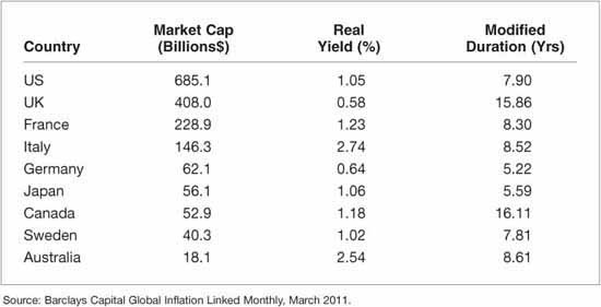
However, there are nuances that differentiate ILBs from one another. International ILBs provide investors with avenues to exploit a variety of currencies, monetary policies, and other local phenomena. These tactical opportunities can be reduced to perspectives regarding absolute global real yield levels, inflation rates, and intercountry differences from these global averages. Exhibit 18–2 reports ancillary data for nine of the larger government issuers of ILBs.
The first and second columns entitled “Market Cap” and “Real Yield” should be of particular interest because they report, respectively, the size and a long-term measure of relative value. Modified duration is simply the sensitivity issues holdings to changes in real yields. Real yield incorporates the return of real principal and the interim real income that an ILBs’ holder will earn.
There are potential international risks not included in Exhibit 18–2 that can affect real yields. The first is the credit profile of the particular issuing country. To the extent that government issuers rarely default on debt instruments denominated in their own currencies, credit risk is low. A second factor is issuance. If a country issues more inflation-indexed supply than domestic and global strategic ILBs investors need, yields are likely to rise until sufficient international tactical investors are attracted.
EXHIBIT 18–2
Data for Nine of the Larger Issuers of Inflation-Linked Bonds
ILBs can be used tactically within equity and cash portfolios as well. Conceptually, the motivation is similar. In the United Kingdom investors often allocate out of equities into ILBs as a defensive tactic—much as U.S. equity managers reallocate defensively into utility stocks to protect against violent market declines.
Strategic Use
Strategic allocations are more deliberate than tactical ones and ultimately speak to the inherent investment qualities of ILBs. ILBs can play a significant role within such top-down strategic allocations. Enduring investor goals, such as matching liabilities, diversifying risks, controlling downside exposures, and achieving real return objectives, typically drive these strategic allocations. In contrast, bottom-up valuation, market timing, and other opportunistic considerations rarely are important aspects of the strategic decision-making process.
Investors typically make strategic asset allocations among the fundamental asset classes: equities, bonds, cash, and inflation hedges. Unadvisedly, some investors opt for finer gradations using more unwieldy sets of narrowly defined asset classes such as large-capitalization, midcap, small-cap equities, and government bonds at the top-level of their asset allocation framework.
Typically, the thread that holds the elements of an asset class together is that each element’s returns are driven primarily by common fundamental phenomena. Simply, correlations between members of the same asset class will be high, whereas correlations between assets that are members of different asset classes will be low.
For ILBs, inflation and real global interest rate are the identifying fundamental phenomena that drive returns. Thus it is reasonable that all ILBs (Treasury, international, agency, and corporate) comprise a distinct asset class, separate from equities, (nominal) bonds, and cash. Real estate, commodities, and certain other “inflation hedges” also fall into this inflation-hedging asset class.
There are three general situations that warrant a strategic reallocation into ILBs. First, portfolio managers looking for higher returns without increased risk may investigate moving out of low-risk assets such as cash. Second, those motivated toward preserving past gains might consider a defensive allocation out of higher-risk assets such as equities or real estate. Importantly, a defensive allocation will tend to decrease or eliminate shortfall probability dramatically. (Shortfall probability is the likelihood that a portfolio will fall below a minimum acceptable threshold.) And third, ILBs can be used strategically in an asset/liability management context.
Asset/Liability Management (ALM)
Asset/liability management is closely related to asset allocation. Traditionally, asset allocation studies do not explicitly incorporate liabilities. They tend to focus on increasing absolute levels of return through allocations to higher-returning assets or through diversification of assets, thereby reducing risk calculated without regard to liabilities.
ALM studies focus on reducing the mismatch between assets and liabilities. Traditionally, researchers have studied ALM in a conventional nominal frame of reference where the exposure of assets and liabilities to conventional yield changes is compared and to some extent matched. Liabilities are assumed to be nominal liabilities even when they are in fact inflation-sensitive.
The large-scale introduction of TIPS by the U.S. Treasury has given asset-liability managers the ability to measure and manage both assets and liabilities that are predominantly real. This is a reprieve for the many investors discussed later.
Investors are not limited to choosing between asset allocation or asset-liability management. The two can be combined into a framework generally termed surplus management—optimizing the return and risk of surplus (assets net of liabilities). Although developed at one asset management firm in the 1970s, this framework comes into and out of favor periodically.
Risk/Return Optimization
The novelty of ILBs as an asset class in the United States poses challenges for strategic users of the securities. In particular, to include ILBs in a standard nominal Markowitz mean-variance optimization, the analyst must input appropriate expected return, variance, and correlation data for ILBs as well as other assets (or liabilities) included in the optimization.
Although conceptually inputs for such optimizations are forward-looking, practitioners usually rely heavily on historical data. Since U.S. TIPS have existed since 1997, correlation matrices are built using asset class returns from 1997 forward or from pro forma estimates of TIPS returns prior to 1997. Although most optimization models function in a nominal frame of reference, some practitioners appropriately implement them in a real frame of reference.
Managing Dedicated ILB Portfolios Using Real Duration
After a ILBs allocation has been determined, an implementation strategy must be executed. For this, an investor chooses between active or passive management. In either case, real duration is a useful metric of exposure because it measures the allocation’s relative sensitivity to changes (parallel shifts) in the real yield curve.
To construct an ILB portfolio, the practitioner needs first to choose a target “real duration” for the portfolio and then to devise a variety of candidate portfolio structures. The candidate portfolios might include a bulleted portfolio having all its ILBs close to the target duration and a barbell portfolio with a combination of longer and shorter ILBs weighted to achieve the target duration.
To select the most advantageous portfolio structure from those with the same real duration, the practitioner need only concern herself with the exposure to changes in the general real yield curve slope of the various candidate portfolios. This is so because the candidate portfolios have the same real yield duration, so their response to parallel shifts will be very similar.
A recent development in the management of TIPS portfolios is increased demand for “break-even” structuring. Typical TIPS portfolios embody inflation protection by locking in to maturity the real yield of instruments owned. Breakeven structuring involves selling similar maturity fixed-rate Treasuries, futures, or paying fixed on interest-rate swaps. This in essence nullifies the real yield and real duration of TIPS, leaving the holder with the inflation indexation of the TIPS held. Of course, realized inflation will need to equal or exceed the inflation which is priced into the nominal market in order to profit from this strategy. In essence this strategy become attractive when (1) real yields are low, so that not much is being given up, and (2) the investor believes that inflation will rise more than what the Treasury market has priced in, or that certain risks are associated with inflation that the investor particularly wants to hedge.
Investor Types: Pension Plans, Endowments, Foundations, and Individuals
Defined-benefit pension plans have both retired-lives and active-lives liabilities. Although ILBs as assets may match the active-life portion of these plans extremely well, plan sponsors typically do not rely exclusively on ILBs to back their active-lives liabilities. Instead, they reach for higher expected returns by using other asset classes with higher risk and return qualities. Given that ILBs and the active-lives liabilities are both linked to inflation,9 sponsors realize that to reach for higher returns, they take on some risk of underperformance in inflationary environments. In addition to generic asset allocations, pension plans may use ILBs to protect a surplus, to offset substantial equity risk exposure, or to reduce the variability of annual funding requirements. Defined-contribution pension plans and their participants also may benefit from the inclusion of ILBs as described separately below.
Endowments, foundations, and other eleemosynary organizations also may have return objectives that are formulated in real terms. Typically their goal is to generate a 5% or higher real return on their investment portfolio. (The IRS generally requires that 5% of a charitable foundation’s assets be spent on the delivery of charitable services each year—so a 5% real return, net of expenses and contributions, is required to maintain the foundation’s inflation-adjusted size.)
Establishing a real-return target for investment performance makes sense for these organizations. Educational or charitable programs, whether they involve physical infrastructure or services, often are budgeted for using inflation-adjusted dollars. Implicitly, such goals, objectives, and plans represent real liabilities.
This suggests that eleemosynaries employ ILBs as a core pillar in their investment strategy. ILBs will not generally achieve 5% returns in isolation, but they go a long way toward engineering out much of the downside risk of return distributions. With the downside risk truncated, more aggressive use of a higher-returning (riskier) asset can be used. As of this writing, eleemosynaries generally have used ILBs only at the margin.
Individuals save primarily to provide for retirement needs and secondarily for children’s education, bequeathment, and other goals. Younger individuals may be relatively immune to the damage that inflation can cause in the context of such liabilities. They hold a large proportion of their “wealth” in the intangible real asset known as human capital (future earning power). As individuals age, the proportion of their real assets typically decrease as their financial assets increase—leaving those in their late 40s and older relatively vulnerable to the inflationary erosion of retirement living standards.
ISSUERS
Although corporations and agencies can and do issue ILBs, governments are by far the largest issuers. By issuing ILBs, government officials make clearer their commitment to maintaining a low level of inflation. A government’s willingness to assume the financial risk of inflation is a powerful signal to the marketplace regarding future policy. Donald T. Brash, governor of the Reserve Bank of New Zealand, characterized this attitude in a speech following New Zealand’s introduction of these securities:
The only “cost” to Government is that, by issuing inflation-adjusted bonds, it foregoes the opportunity of reducing, through inflation, the real cost of borrowing . . . Since [the New Zealand] Government has no intention of stealing the money invested by bondholders, foregoing the right to steal through inflation hardly seems a significant penalty.10
How can an investment instrument that makes so much sense for investors, as described in preceding sections, also be advantageous to the issuer? Brash’s quote provides one example of how investors gain while the issuer forfeits something it considered worthless to begin with. Next we discuss the U.S. Treasury rationale for issuing TIPS.
U.S. Treasury’s Rationale
A goal of the Clinton administration was to reduce the future interest burden of the Treasury’s debt. Balancing the budget was the main target of this policy, but a secondary objective took aim at “bond market vigilantes.” The administration recognized that because of the “maturity premium” inherent in longer-term debt, rolling over a 3-year bond ten times likely would incur less interest cost than issuing a single 30-year bond. One of the most important programs Treasury embarked on during this administration was a deliberate effort to reduce the average maturity of outstanding debt.
TIPS Program
The TIPS program was instituted in this spirit. Like floating-rate debt, TIPS have long stated but short effective maturities, reducing the “rollover risk” inherent in short-term debt. Additionally, TIPS explicitly provide market-based inflation forecasts for use by the Fed. TIPS reduce the expected cost of financing a government’s debt because they are conceptually free of the inflation risk premium built into nominal long-term bond yields. Normally one might conclude that by relieving bond investors of this risk, the Treasury implicitly absorbs a burden or risk equal in magnitude. This is not the case here, however.
By reducing nominal debt and increasing inflation-indexed (real) debt, the Treasury has in effect changed the structure of its liabilities to better match its only asset—its authority to tax. Put another way, the Treasury is the ideal issuer of inflation-indexed debt.
The issuance of TIPS improves taxpayer welfare by eliminating the 0.5% to 1.0% inflation risk premium that researchers believe is embedded in nominal bond yields. At the margin, investors are indifferent to accepting lower yields versus living with the higher risk of nominal debt—so conceptually they are no better or worse off. The elimination of this inflation risk premium is therefore a true welfare gain. In practice, the welfare gains of issuing TIPS have been split between issuers and the investors.
Moral Hazard
The government is both the issuer of TIPS (Department of Treasury) and publisher of the CPI (BLS, Department of Labor). The inherent ambiguity in measuring the CPI creates a moral hazard because the government can directly control the economic value of its liability. Fortunately, several factors mitigate the risk of the government publishing statistics that are not scientifically based.
First, professional integrity, a strong institutional infrastructure, and influential political constituencies combine to preclude the government from manipulating the CPI. Second, any confiscation of value through index distortions would be perceived by the financial community as an erosion of credibility or, if blatant, tantamount to default. Since the issuance process is a repeated game of substantial proportion, such an erosion of credibility would have long-term repercussions on future debt issuance and other government promises that would greatly outweigh any apparent short-term economic or political benefits.
International Issuers
The ILB market in the United Kingdom is large and well developed, comprising about 20% of outstanding debt. Additionally, Canada, Australia, France, Italy, and Sweden have issued ILBs in large enough quantities to ensure reasonable market liquidity as well.
While each of these countries shares the basic inflation-protection concept with their U.S. cousins, differences include market size, trading liquidity, time lag associated with the inflation indexation, taxation, day-count conventions, and quotation conventions. These differences substantially influence both observed quoted real yields and “true” real yields available to investors.
All the ILBs issued by these six governments, together with those issued by the U.S. Treasury, make up a performance benchmark of liquid global inflation bonds known as the Barclays Capital Global Inflation-Linked Bond Index.
Corporate Issuers and CPI Floaters
In addition to the U.S. Treasury and non-U.S. government issuers, U.S. corporations, agencies, and municipalities have issued inflation-indexed bonds. Two of the earliest corporate issuers were the Tennessee Valley Authority and Salomon Brothers. Their inflation-indexed bonds were virtually identical in structure to U.S. Treasury TIPS. Other issuers, including Nationsbank, Toyota Motor Credit, the Student Loan Marketing Association (SLMA), and the Federal Home Loan Bank (FHLB), have chosen to structure their bonds as CPI floaters.
A CPI floater is a hybrid between TIPS and a conventional floating-rate note (FRN). Like a TIPS, its return is closely linked to CPI inflation. Like a conventional floating-rate note, its principal is fixed in size. The coupon rate of a CPI floater fluctuates and is typically defined as the CPI inflation rate plus a fixed-percentage margin.
OTHER ISSUES
Taxation
U.S. TIPS are taxed similarly to zero-coupon bonds. They incur a tax liability on phantom income (income earned but not paid.) This does not mean that investors in TIPS pay more taxes or that they pay taxes sooner than holders of nominal bonds. In fact, if inflation, nominal yields, and tax rates are constant, the cashflow profile of taxes paid and payments received on TIPS is comparable with those of nominal bonds (assuming reinvestment of the excess coupon). In practice, many taxpayers hold TIPS in tax-exempt accounts (401(k)s, etc.) or within mutual funds (which are generally required to distribute taxable income).
Deflation Protection
Questions naturally arise regarding how TIPS would behave in a deflationary environment (one where prices are literally falling). Applying CPI indexation, the current adjusted principal value would be less than the prior adjusted principal value. This would affect semiannual interest payments accordingly.
Extending this premise, it is certainly possible for the adjusted principal value to fall below the original principal value—and therefore for coupon payments to be calculated on a shrinking base. Note that they would still be positive and almost equal to their original size. For example, even after 10 years of 1% deflation and a resulting price level that was 10% lower than when it started, the semiannual coupon payments on a $1,000 TIPS would still be about $18 (rather than $20 originally). The final principal repayment would be treated even more favorably.
In particular, the Treasury has guaranteed that for the maturity payment of principal (and only the maturity payment), the investor will not receive less than the original principal amount.
In such deflationary circumstances, in order to maintain acceptable nominal returns, the Treasury would in effect be paying a higher real return than initially promised. The Treasury decided that the regulatory, institutional, and psychological benefits of providing this guarantee would facilitate distribution of the bonds to an extent that more than justifies the theoretical contingent cost to the government.
This government guarantee of 100% principal return distinguishes TIPS from all other inflation hedges.
KEY POINTS
• The inflation indexed bond market has existed for centuries in various forms, but blossomed in 1997 when the U.S. Treasury introduced Treasury Inflation-Protected Securities or TIPS, and in years since as investors have adopted them strategically.
• The market real yield on TIPS can be subtracted from the market nominal yield of similar maturity fixed-rate Treasuries to arrive at the “break-even inflation rate.”
• A broad range of investors incorporated TIPS into their asset allocations in order to lock in fixed real yields, while protecting their principal from erosion of purchasing power.
• Currently investors utilize a “break-even” structure in determining their allocations to TIPS. This involves hedging out the relatively low real yields currently priced by the market in order to profit more directly from a rise in inflation, which may or may not be accompanied by rising real yields.