
CHAPTER TWO
WAREHOUSE ACTIVITY PROFILING, DATA MINING, AND PATTERN RECOGNITION
2.1 The P’s and P’s of Profiling
2.2 Warehouse Activity Profiles
Imagine that you were sick and went to a doctor for a diagnosis and prescription. When you arrived at the doctor’s office, he already had a prescription waiting for you, without even talking to you, let alone looking at you, examining you, or doing blood work. In effect, he wrote your prescription with his eyes closed and a random prescription generator. Needless to say, you would not be going back to that doctor for treatment.
Unfortunately, the prescriptions for many sick warehouses are written and implemented without much examination either. For lack of knowledge, lack of tools, and/or lack of time, many warehouse projects launch without any understanding of the root cause of the problems and without exploration of the real opportunities for improvement.
Warehouse activity profiling and data mining is the systematic analysis of item and order activity, seeking to identify and take advantage of patterns of opportunity. Our pattern recognition algorithms highlight the root cause of material and information flow problems, pinpoint major opportunities for process improvements, and provide an objective basis for project-team decision making.
I will start with some of the major motivations and potential roadblocks to successful profiling. Then I will review a full set of example profiles and their interpretations. The examples will serve to teach the principles of profiling and as an outline for the full set of profiles required for warehouse reengineering.
2.1 The P’s and P’s of Profiling
I have been leading, facilitating, researching, and teaching activity profiling and data mining for more than 20 years. I recently summarized our lessons learned as the P’s and P’s of profiling.
The Preparation of Profiling
The first thing I do before writing a new article is to read what others have written about the topic. If I am preparing to teach a class or a seminar, I do the same thing: I review what others have prepared on the topic to stimulate my thinking. Reviewing activity profiles works the same way; it is like reading an illustrated journal of the warehouse activity. As you study the profiles of customer orders, purchase orders, item activity, inventory levels, and so on, the creative juices should begin to flow as your understanding of underlying activity improves.
The Power of Profiling
Done properly, the patterns in profiling quickly reveal a small set of candidate process flows and material handling equipment types for each warehouse activity. Conversely, profiling quickly eliminates process and equipment options that really do not warrant consideration. Many warehouse reengineering projects go awry because we waste valuable resources analyzing concepts that were doomed from the start.
The Participation of Profiling
Profiling involves key stakeholders. During the profiling process, it is natural to ask people from many affected groups to provide data, to verify and rationalize data, and to help interpret results. To the extent those stakeholders have been involved, they have helped with the design process.
The Probity of Profiling
Profiling supports and promotes objective decisions. I worked with one client whose team leader we somewhat affectionately called “Captain Carousels.” No matter what the data said, no matter what the order and profiles looked like, no matter what the company could afford, he was going to have carousels in the new design.
The Purpose of Profiling
You will see myriad complex statistical distributions in our journey through warehouse activity profiling. Why go to all the trouble?
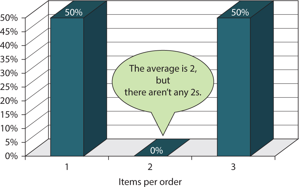
Suppose that we are trying to determine the average number of items on an order. Figure 2.1 shows that 50 orders are for one item, 0 are for two items, and 50 are for three items. What is the average number of items per order? It’s two. How often does that happen? It never happens! If we are not careful to plan and design based on distributions as opposed to averages, our plans and designs will be flawed.
Figure 2.1 Items per order distribution completed for a small mail-order company. The average is two lines per order, but the average never happens.
The Principal and Principle of Profiling
Vilfredo Pareto was an Italian economist and gardener. Pareto’s law stems from his observation that 80 percent of the land was owned by 20 percent of the population and that 20 percent of the peapods in his garden yielded 80 percent of the peas. Joseph Juran called this principle the “separation of the vital few from the trivial many.” Activity profiling and data mining are essentially the repeated and logical application of Pareto’s law, sometimes referred to as the 80/20 principle or ABC analysis. Examples of Pareto’s law working in warehousing include
![]() A minority of the items generate a majority of the activity.
A minority of the items generate a majority of the activity.
![]() A minority of the items are responsible for a majority of the inventory.
A minority of the items are responsible for a majority of the inventory.
![]() A minority of the customers generate a majority of the picking and shipping activity.
A minority of the customers generate a majority of the picking and shipping activity.
The Pictures of Profiling
When you see a picture you experience a thousand simultaneous thoughts. We are aiming for the same effect in warehouse activity profiling as we paint a representative picture of warehouse activity. In profiling, we capture the activity of the warehouse in pictorial form so that we can quickly develop wise, data driven, consensus decisions.
The Perspectives of Profiling
If a picture is worth a thousand words, then a video is worth a thousand pictures. Interactive data visualization, simulation, and animation are the closest media we have to video for activity profiling. Interactive data visualization (Figure 2.2) is simply dynamic charting controlled by the user. Simulation (Figure 2.3) is typically a two-dimensional representation of the physical warehouse with the activity profiles moving warehouse objects according to the profiles. Animation (Figure 2.4) is three-dimensional simulation.
Figure 2.2 Interactive warehouse data visualization for a large consumer products company.
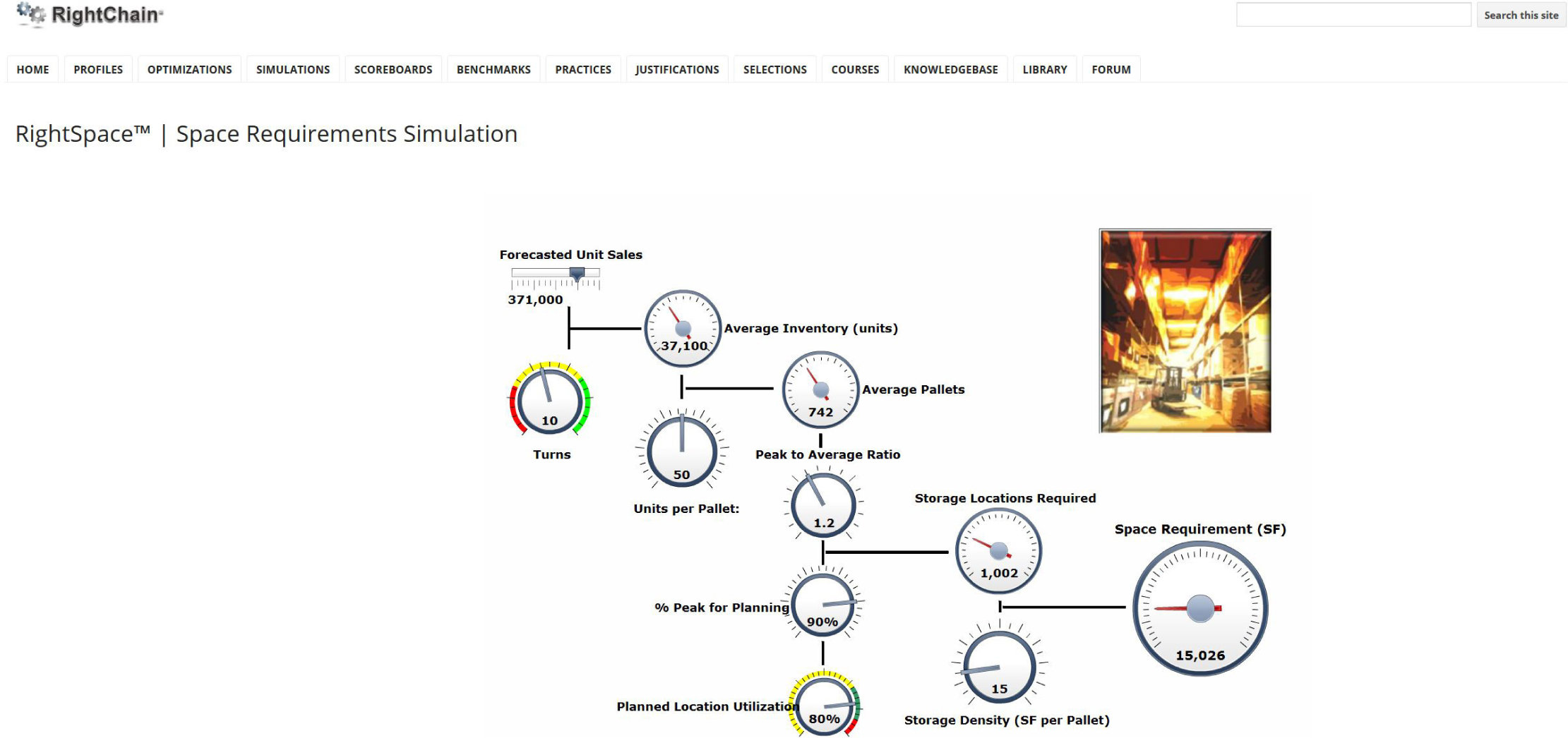
Figure 2.3 Two-dimensional warehouse simulation for a large pharmaceutical company.
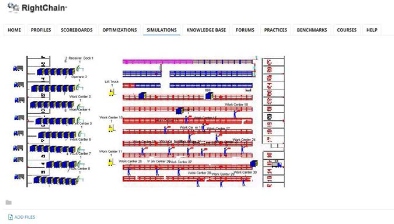
Figure 2.4 3D animation model of a large cosmetics distribution center.

The Pitfalls of Profiling
One warning before we begin to profile the warehouse (as an engineer and logistics nerd, I fall into this trap a lot): We can drown in our own profiles. Some people call this paralysis of analysis! If we are not careful, we can get so caught up in profiling itself that we forget to solve the problem.
2.2 Warehouse Activity Profiles
Over the years we have developed a structured and comprehensive suite of activity profiles to address the major planning, design, and management decisions in a supply chain strategy. The profiles are constructed with our proprietary pattern recognition algorithms and are fed from a supply chain data warehouse (Figure 2.5). The warehouse activity profiles are organized according to Figure 2.6.
Figure 2.5 RightChain™ Decision Support Suite.
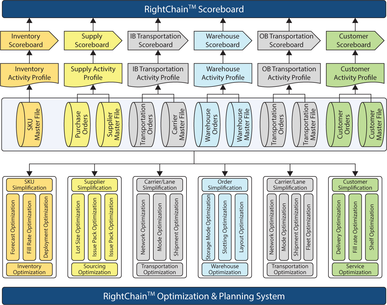
Figure 2.6 Warehouse activity profiles.
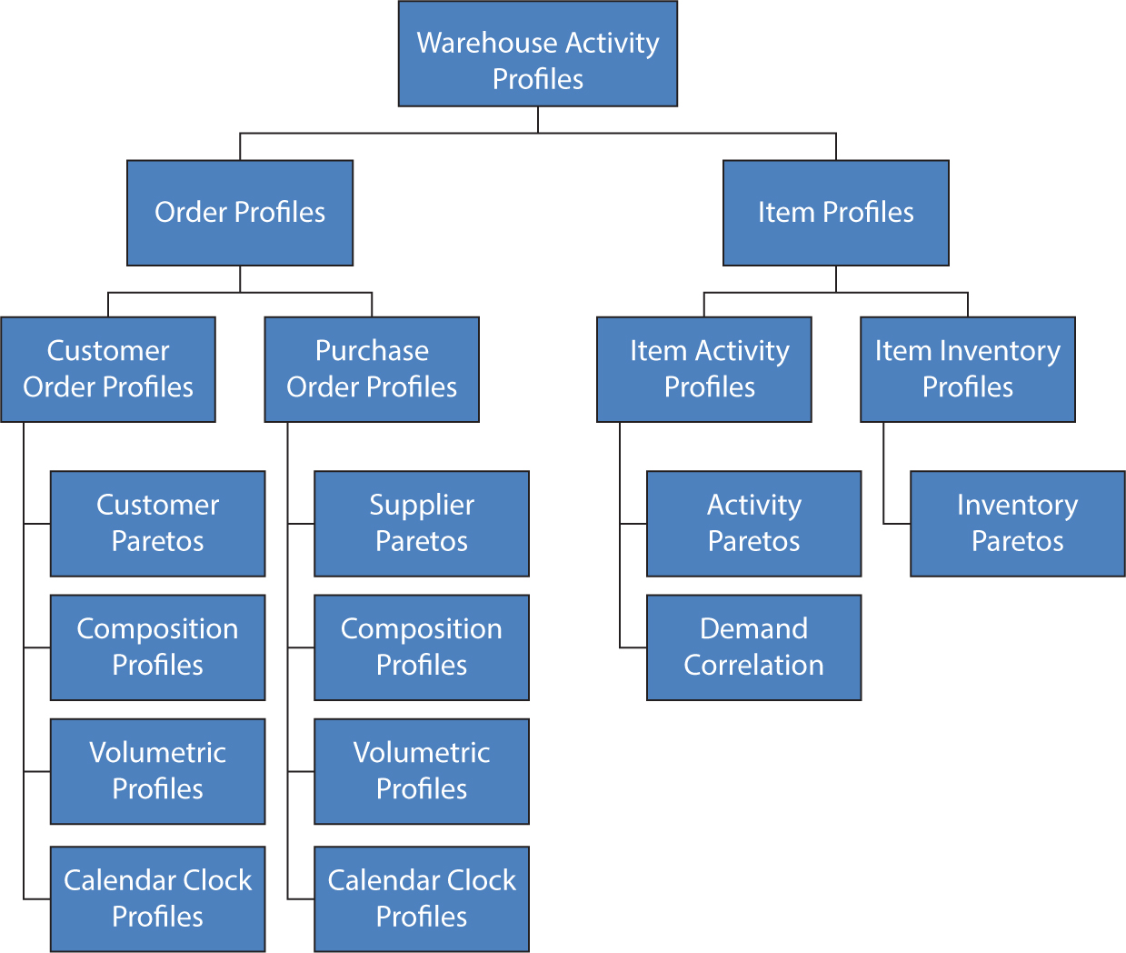
Order Profiles
Order profiles include customer order profiles, purchase order profiles, and inbound/outbound transportation order profiles. They jointly portray the major patterns of warehouse activity. Time and space do not permit a full description of each of the four major profiles. I selected customer order profiles as the context for our presentation on order profiles.
Material and information should flow through a warehouse to facilitate excellent customer service. What do customers really want from a warehouse? They want their orders filled in an accurate, timely, and cost-effective manner. Accordingly, the first thing we must understand to plan and design warehouse operations is the profile of customers and their orders.
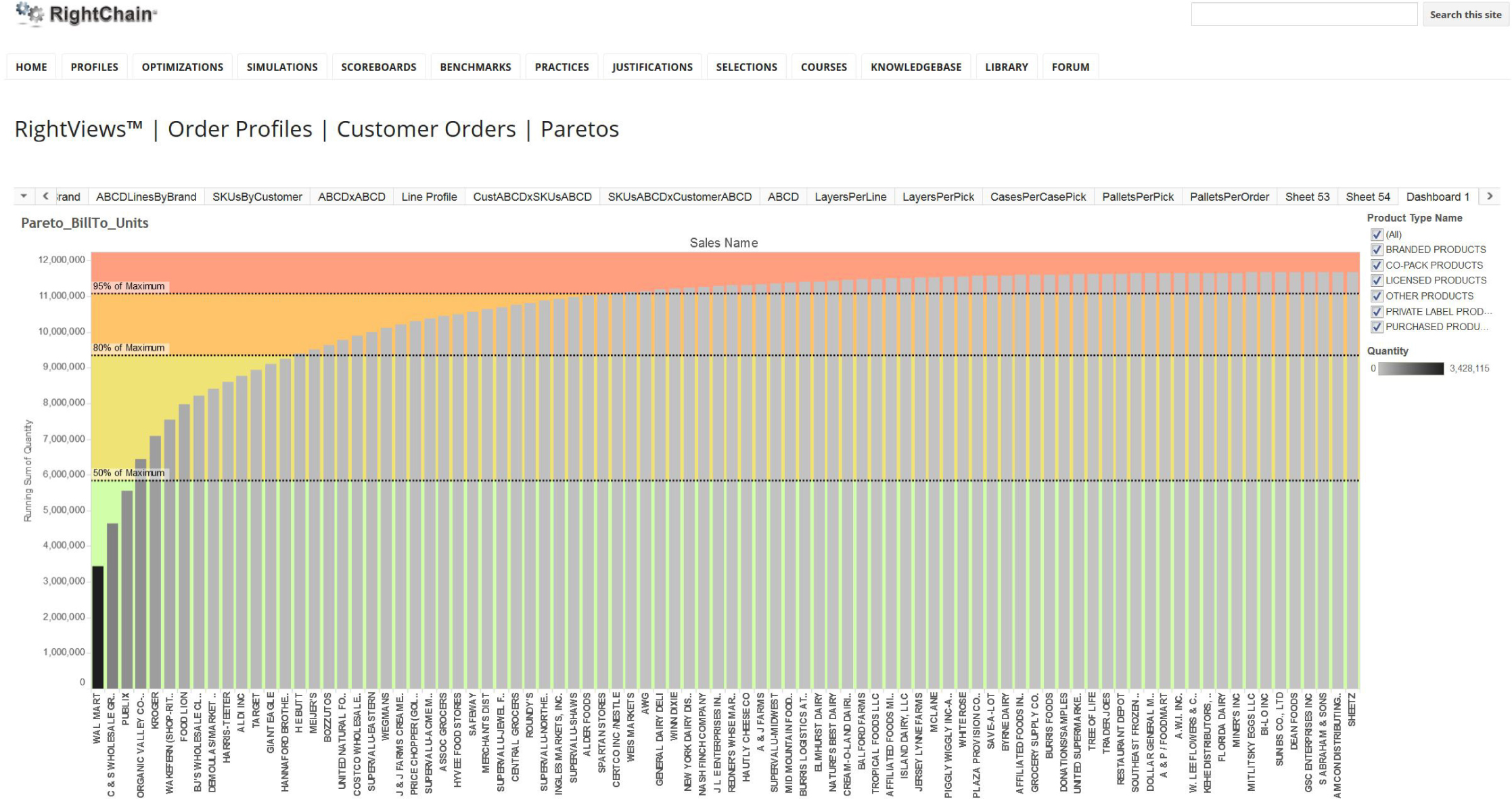
Customer Paretos
Some customers place such high demands on a warehouse, represent such a large portion of the activity of the warehouse, and have such demanding customer-service requirements that it may make sense to establish a separate area within the warehouse for those customers. For example, one of our apparel manufacturing clients does so much business with JC Penney that they have a JC Penney warehouse within their warehouse. It is not uncommon for consumer products and food manufacturing companies to have areas within their warehousing dedicated to Wal-Mart activity.
The customer pareto in Figure 2.7 is from one of our food and beverage clients. Note that just three customers make up 50 percent of our client’s distribution center activity. Accordingly, we assigned each of those customers their own zones in the warehouse to reduce travel time and improve customer service.
Figure 2.7 A small minority of customers generate a large majority of picking and shipping activity.
In another example (Figure 2.8), in a large publisher’s distribution center, a central pool of reserve stock is used to support three distinct internal customers/business units—retail, trade, and periodicals. We designed the central, shared warehouse with allocated, random storage and the forward picking areas with dedicated, distinct forward picking zones. The manager of each forward picking zone has a dotted-line reporting relationship with the business unit to which his or her picking zone reports. The solid-line reporting relationship is to the director of distribution. This warehouse-within-a-warehouse design yielded the best of both worlds—shared receiving resources, efficient handling of central inventory, dedicated forward picking lines, shared shipping resources, and business unit accountability.
Figure 2.8 Warehouse-within-a-warehouse concept developed for a large publishing company.

The warehouse-within-a-warehouse design philosophy works because small warehouses, in general, have higher productivity, response time, and accuracy performance than large warehouses. Many of the customer-order and item-activity profiles identify opportunities to subdivide a warehouse operation into self-contained warehouse processing cells, virtual warehouses, or warehouses within the warehouse. A warehouse within a warehouse is similar to a flexible manufacturing cell in a factory, where the productivity, quality, and cycle time are much better than in the factory as a whole.
Composition Profiles
Customer order composition profiles include the following:
![]() Family-mix profiles
Family-mix profiles
![]() Handling-mix profiles
Handling-mix profiles
![]() Order-increment profiles
Order-increment profiles
Family-Mix Profiles The overall operating strategy of a warehouse should be influenced by the extent to which orders require items from multiple families. If the majority of the orders are pure, drawing from a single product family, then zoning the warehouse on that basis could create virtual warehouses within the warehouse.
For example, the family-mix profile in Figure 2.9 was developed for a wholesale distributor of fine papers, copy/laser paper, and envelopes. Printers make high-quality brochures from flat stocks of fine papers. A carton of flat stock is 30 inches long, 24 inches wide, and 9 inches deep. A carton weighs 80 pounds. Cut stock is basic 8½- by 11-inch copier and laser printer paper. A carton of cut stock is 24 inches long, 10 inches wide, and 10 inches deep. A carton weighs 20 pounds. The third product family is envelopes—extremely small and lightweight merchandise.
Figure 2.9 Family-mix profile for a large paper distributor.
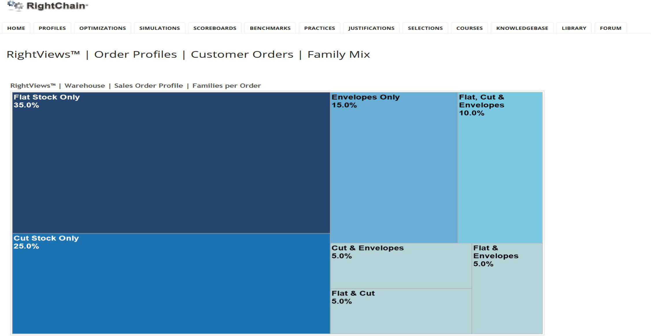
In this example (Figure 2.9), we are evaluating the merits of zoning based on those three product families—flat stock, cut stock, and envelopes. If the orders are mixed—that is, flat stock, cut stock, and envelopes tend to appear together on customer orders—then in pallet building, we would start with flat stock, put cut stock on top of that, and put envelopes on top of that. If we zone the warehouse that way, we may pay a big travel-time penalty passing pallets between those zones. However, if the orders are pure—that is, they tend to be “complete-able” out of a single product family—then zoning the warehouse by product family will establish efficient warehouse processing cells, especially since inbound loads already arrive in those same product families.
In Figure 2.9, 35 percent of the orders can be completed solely from flat stock items, 25 percent can be completed solely from cut stock items, and 15 percent can be completed solely envelope items. The good news is that 75 percent of the orders (35 percent + 25 percent + 15 percent) can be completed within a single product family. Zoning the warehouse based upon those families yielded a 38 percent increase in overall operating productivity.
Handling-Mix Profiles The full/partial-pallet mix profile and the full/broken-case mix profile are two handling-unit mix profiles.
Full/Partial-Pallet Mix Profile With a full/partial-pallet mix profile, we determine whether full and partial pallet picking should take place in the same or separate areas. For example, in Figure 2.10, 52 percent of the orders are “complete-able” out of partial-pallet quantities, that is, just case picks; 29 percent of the orders are “complete-able” from full-pallet quantities, and the remaining 19 percent of the orders require both partial- and full-pallet quantities. The profile strongly suggests that separate areas for full and partial picking should be established.
Figure 2.10 Full/partial-pallet mix profile for a large office supplies company.
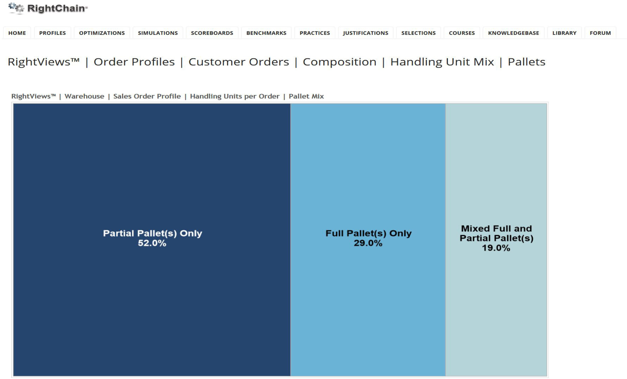
Should we have separate case picking and pallet picking areas? If so, would we pay a big penalty for mixed orders that require merging of the partial- and full-pallet portions of the order? No, only a small minority of the orders are mixed. For 81 percent of the orders, zoning based on pallet/case picking creates warehouses within-the-warehouse. When the orders are released into the warehouse management system, it should classify them immediately as pallet pick orders, carton pick orders, or mixed orders. For mixed orders, the warehouse management system should create a pallet portion and a case pick portion and either pass the full-pallet portion to the case pick area or merge the case pick and pallet portions downstream from picking.
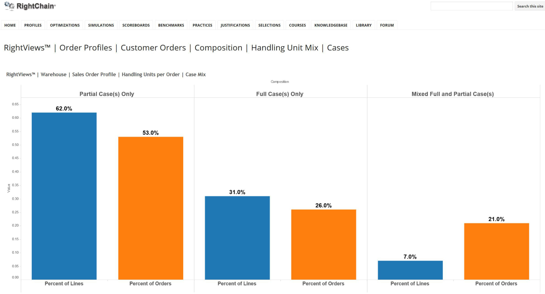
Full/Broken-Case Mix Profile The full/broken-case mix profile helps us determine whether we should create separate areas for full- and broken-case picking. As was the case with the pallet/case-mix profile, the profile in Figure 2.11 indicates that only a small portion of the orders requires both a full- and broken-case quantity. Hence, creating separate areas for full- and broken-case picking will yield two order-completion zones with very little mixing between them.
Figure 2.11 Full/broken-case mix profile.
Order-Increment Profiles Order-increment profiles (Figure 2.12), illustrate the portion of a unit load (in this situation, a pallet) requested on a customer order. For example, suppose that there are 100 cartons on a pallet and a customer orders 50 cartons. In this case, the customer ordered 50 percent of the pallet. If there are 80 cartons on a pallet and that customer orders 20, they ordered 25 percent of the pallet.
Figure 2.12 Pallet order-increment distribution for a large office supplies distributor.
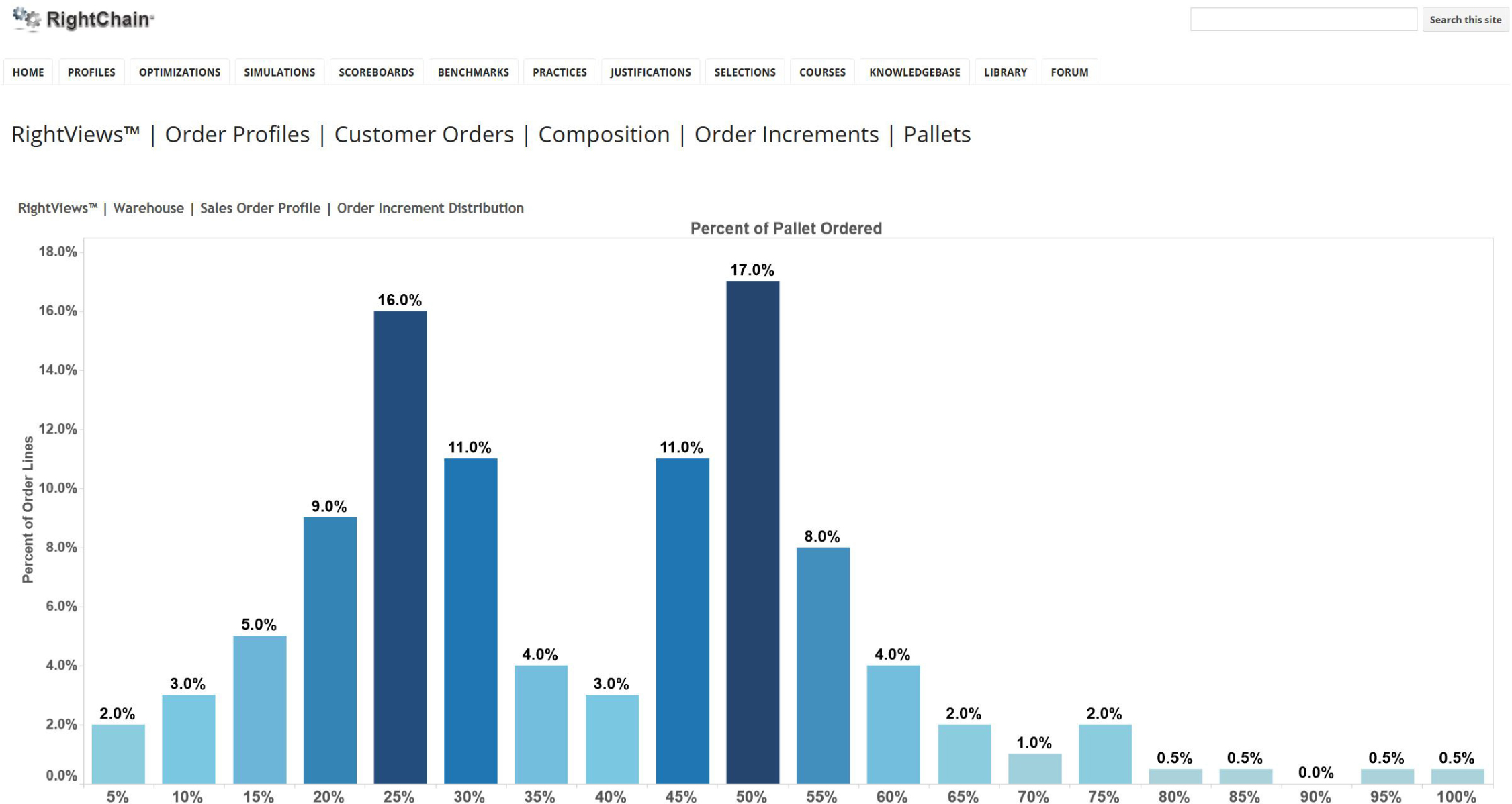
What do you notice that is unusual about this distribution? (In almost all these distributions, the key insights are in the peaks and valleys). Where are the peaks? The peaks are around 25 and 50 percent of a pallet.
Suppose that there are 100 cartons on a pallet and a customer places an order for 100 cartons. Would you rather pick a full pallet or 100 individual cartons? You did not have to read this book to figure out that you would prefer to pick a whole pallet at a time. In addition, a customer would rather receive a full-pallet quantity that they can handle in one unit load as opposed to having to handle 100 loose cartons.
How can we build half- and quarter-pallet unit loads? In this particular case, the manufacturing facility is attached to the warehouse. There is a palletizer that sits on the border, and all we have to do is set the palletizer to put a pallet in place about four times as often as it builds quarter pallets and twice as often as it builds half pallets. If the warehouse is not attached to a manufacturing facility, the next-best scenario is to have the supplier build the quarter- and half-pallet loads. And if not the supplier, then we can preconfigure the unit loads at receiving.
Can we influence customers to order in half-, quarter-, and/or layer-quantity increments? Absolutely! In many cases, simply by making the pallet/layer quantities accurate and visible to the customer and the order-entry personnel, we can encourage the practice of ordering in preconfigured-unit loads. We can further encourage the practice by offering price discounts designed around efficient handling increments. In this case, there was a representative from the sales organization on the cross-functional team who literally reset the price breaks on the quarter- and half-pallet quantities the next day. Picking productivity increased by 68%.
The two potential downsides of preconfiguring sub-pallet unit loads are (1) the complications of strict product rotation requirements rotation requirements and (2) loss of storage density. I believe that in many industries first in, first out FIFO requirements are exaggerated. For example, I recently worked with a candy company that continued to hold out FIFO as a barrier to productivity improvements. I can remember a design meeting on Valentine’s Day when our client was receiving product for the Halloween season. There can be some large time windows within FIFO requirements.
There will be some loss in storage density because a pallet worth of cartons may now have two or four pallets supporting it. For half-pallet quantities, we should be able to stack two halves in a full opening. For quarter-pallet quantities, we may need a row of openings that are 15 percent taller than the opening for singles. As a result, the loss in storage density should be less than 5 percent for the entire warehouse.
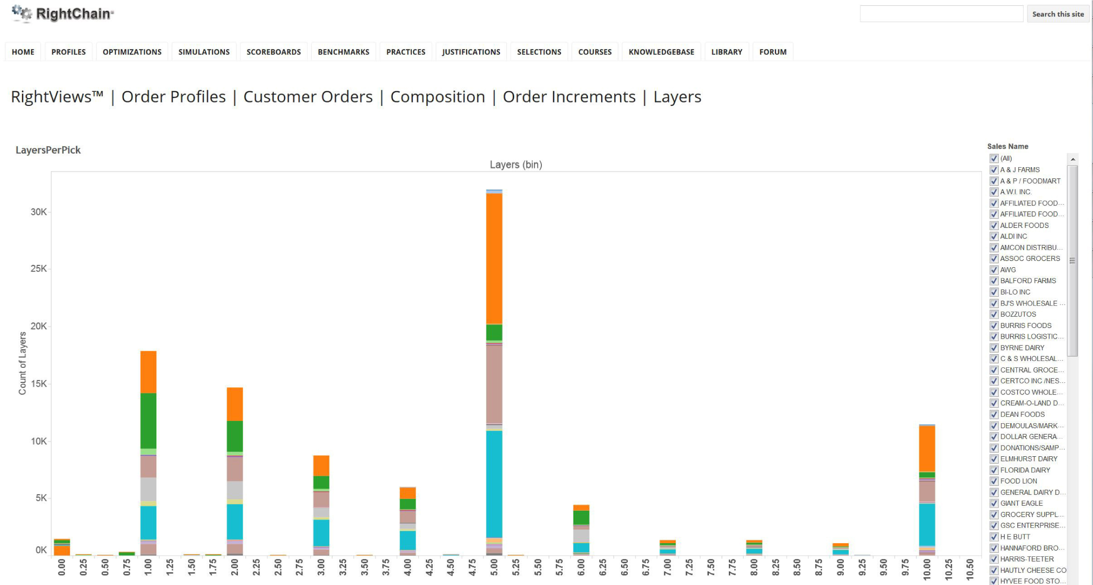
Layer Picking Customers often order in full layer quantities. An example from a food and beverage client is illustrated in Figure 2.13. Note that 80 percent of the order lines are for full-layer increments, leading to our strong recommendation that layer picking be implemented to dramatically increase the productivity and throughput capacity. (A variety of layer picking systems are described in Chapter 6.)
Figure 2.13 Layer picking profile for a large food and beverage company.
Split Case Inner Packs The case order-increment profile (Figure 2.14), determines the portion of a full carton that is requested on customer orders. For example, if there are 100 pieces in a carton and a customer orders 50, the customer ordered half the carton. What do you notice that is unusual about this profile? In this example, customers tend to order around half a carton and a quantity close to a full carton. As a result, we would like to set price breaks at a half carton (and create an inner pack for a half carton) and at a full carton to encourage customers who are almost ordering that quantity to order in full-carton increments.
Figure 2.14 Case order-increment distribution for a large pharmaceuticals firm.
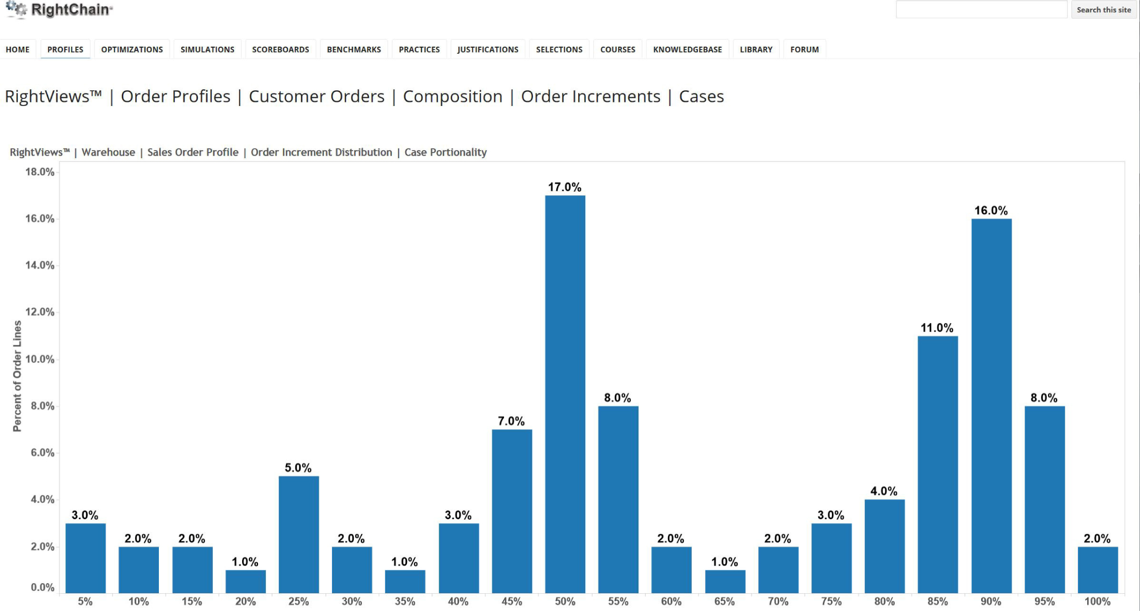
The general principle is to prepackage in increments that customers are likely to order in and to encourage customers to order in those increments. Ideally the supplier should do as much as possible to help prepare the product for picking and shipping. Then we should do as much as possible at the receiving dock to prepare product for shipping immediately upon receipt as we have the longest time window available for picking/shipping preparation. As soon as an order drops for that product, the handling and preparation of the product for shipping should be minimized.
Customer Order Volumetric Profiles Our customer order volumetrics include lines-; units-; cube-; and weight-per-order profiles; and joint profiles comprised of the same. Some sample profiles are provided below.
Lines-per-Order Profile The lines-per-order profile portrays the number of unique stock-keeping units (SKUs) on an order. It is one of the most important profiles because each unique SKU or line on an order represents a visit to the unique location for that SKU. Location visits are the majority of the workload in any warehouse. Consequently, managing location visits is perhaps the master key to maximizing warehouse productivity.
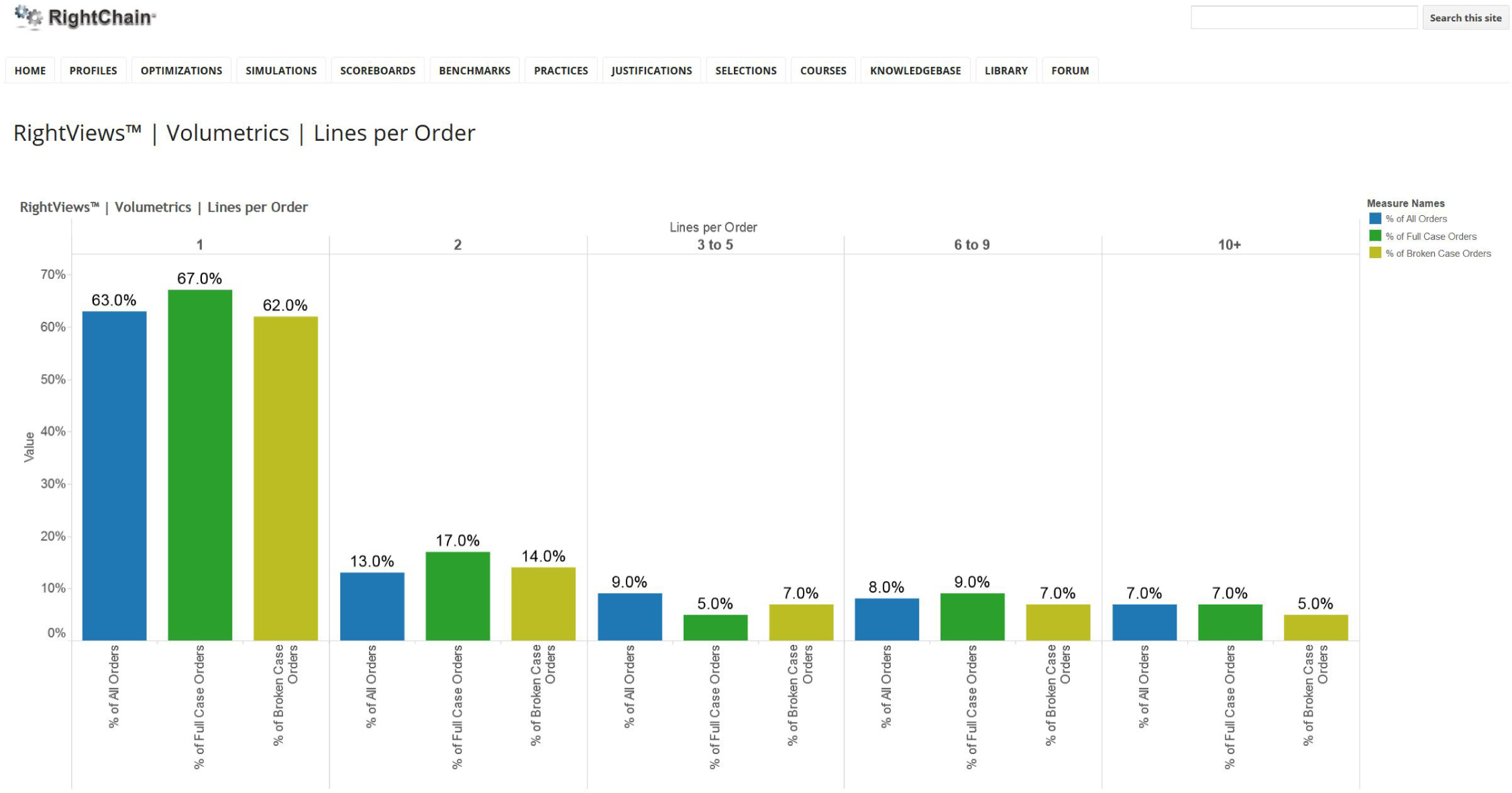
The lines-per-order profile in Figure 2.15 indicates that 63 percent of the orders in the warehouse are for one line item, 13 percent for two, 9 percent for three to five, 8 percent for six to nine, and 7 percent for 10 or more. Where is the peak? It is around single-line orders. This distribution is common in the mail-order industry or when individual consumers or technicians order directly for a warehouse. We now need to consider the operating strategies that take advantage of this order profile.
Figure 2.15 Lines-per-order distribution for a large mail-order company.
Singles may be back orders. Back orders are an excellent opportunity for cross-docking. Singles may be batched together for picking on single-line picking tours. By presenting single-line orders in location sequence, we create very efficient picking tours. In addition, the single-line order batches naturally break the warehouse into zones defined by the length of the picking tour. Single-line orders also may represent an opportunity to create a dynamic forward pick line. In this operating scenario, an automated look-ahead into the day’s or shift’s orders may yield a number of SKUs for which there is at least a full carton’s worth of single-line orders. Those SKUs can be batch picked and set up along fast pick-pack lines.
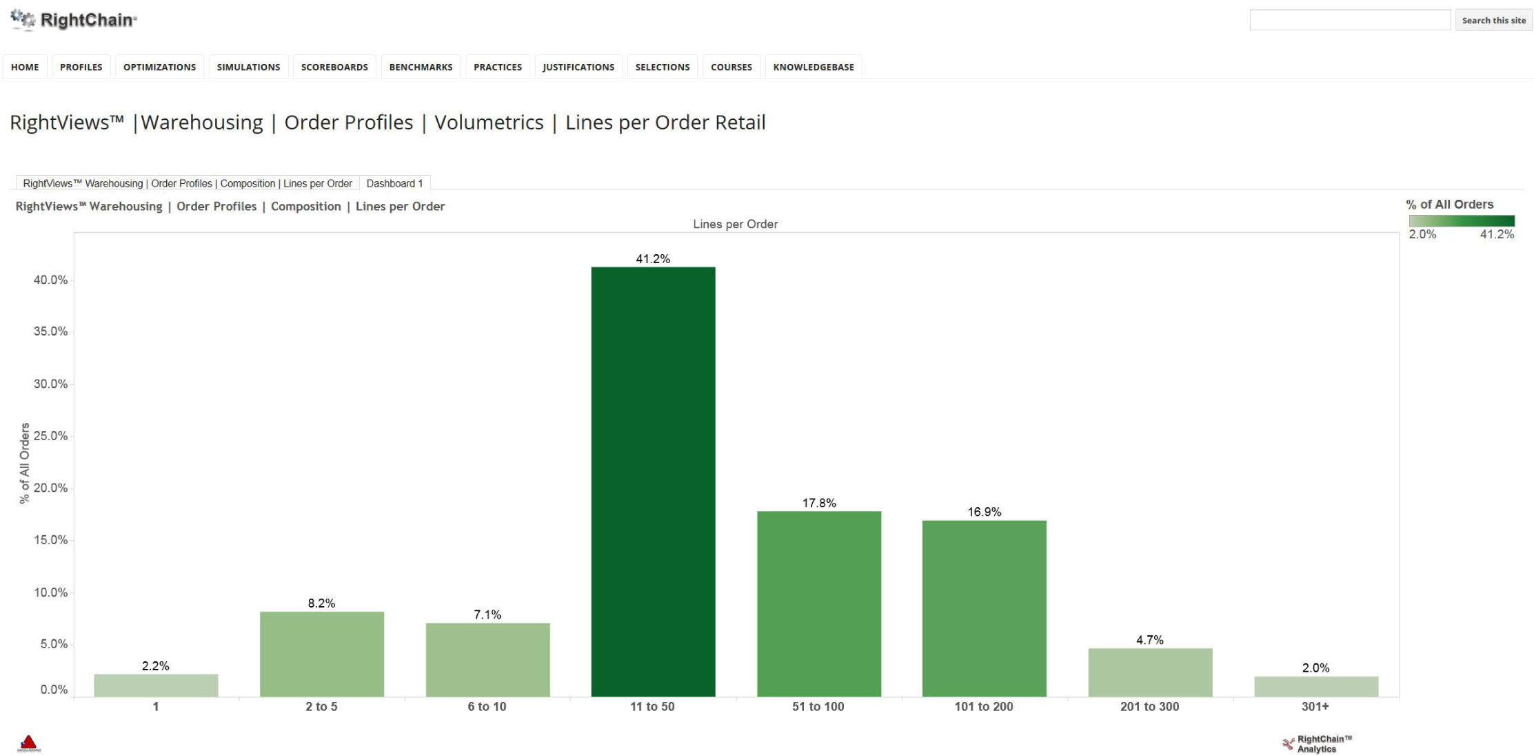
Another common lines-per-order profile is illustrated in Figure 2.16. The peak is around 10+ lines per order. This profile is common in retail/grocery/dealer distribution, where the customer is a retail store/grocery store/dealership. In this case, there is typically enough work to do within an order that the order itself represents an efficient work set. Or the order may be so large that it may be split across multiple order fillers for zone-wave picking.
Figure 2.16 Retail lines-per-order profile for a large convenience store chain.
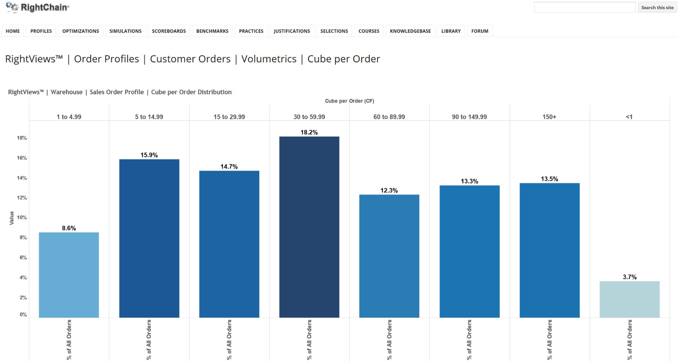
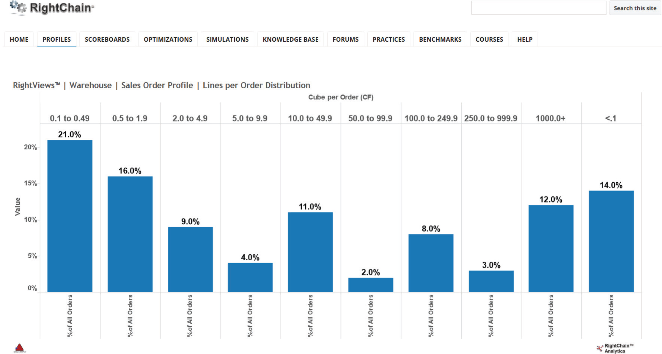
Cube-per-Order Profile The cube-per-order distribution (Figure 2.17) illustrates the portion of outbound orders falling into pre-defined cube classifications. It may suggest alternative sizes for shipping containers, alternative picking methods, alternative transportation modes, and requirements for staging space. The figure depicts a cube-per-order distribution for a large toy company client. We use the profile to help select picking methods and container sizes for their mix of picking tours.
Figure 2.17 Cube-per-order profile for a large toy company.
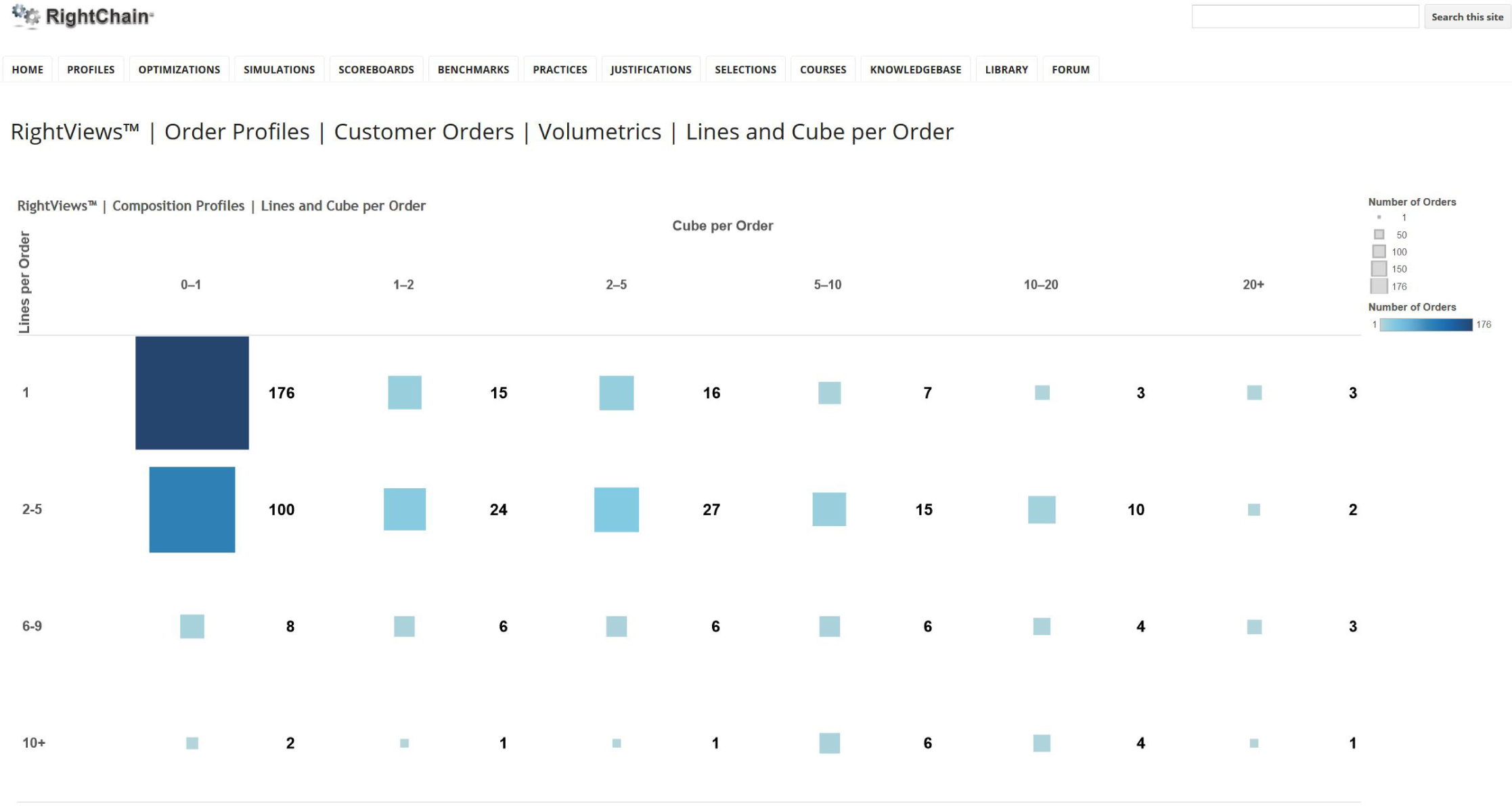
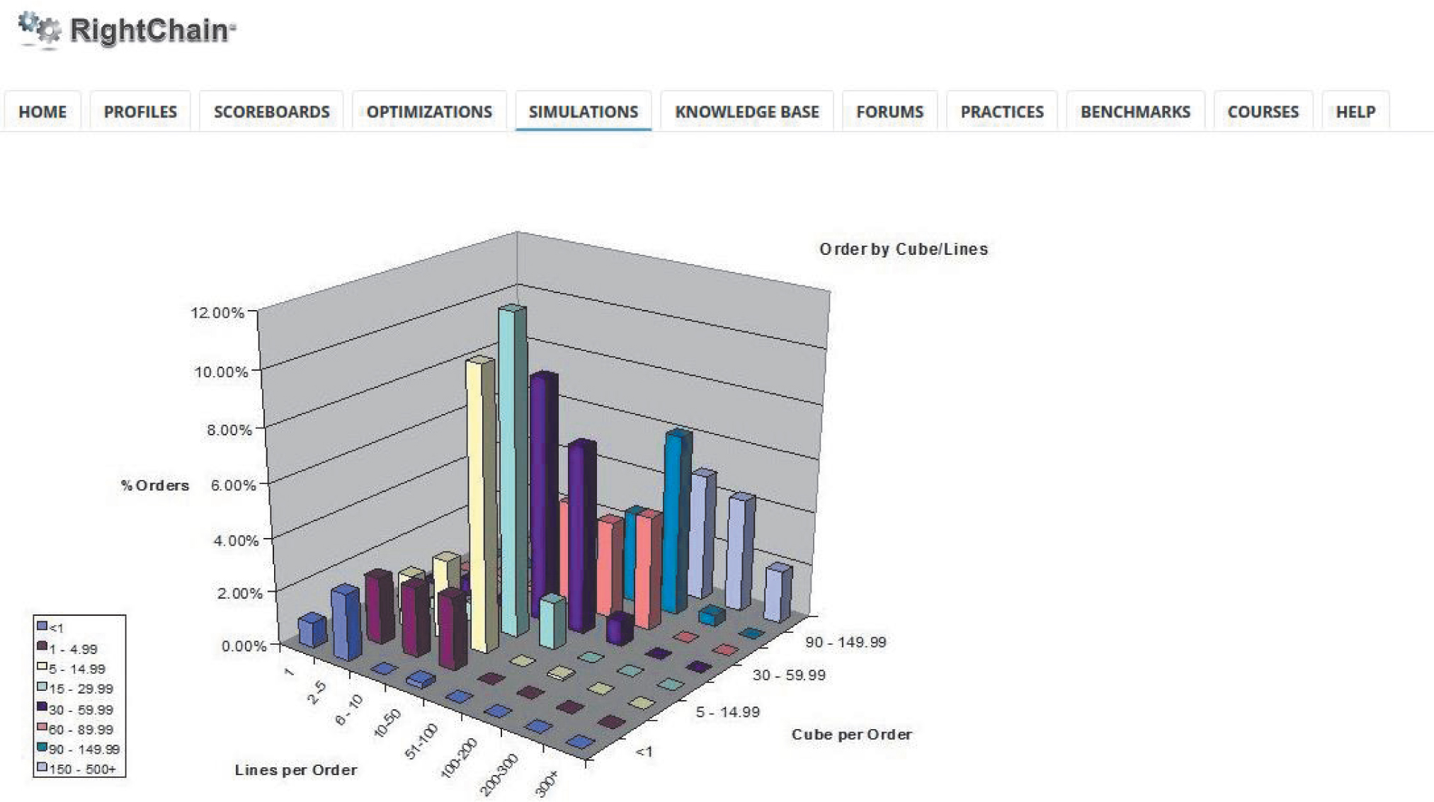
Lines- and Cube-per-Order Profile The lines- and cube-per-order profile (Figure 2.18) brings together in one profile the critical information needed to define order picking strategy. It is a joint distribution that classifies all orders into lines-per and cube-per families. In this example, there are 176 orders with one line item and that occupy less than a cubic foot of space. These orders are probably candidates for a single operator to batch together for picking into compartmentalized picking carts, totes, or shipping containers. There is one order with more than 10 line items that occupies more than 20 cubic feet, about a third of a pallet. That order is a candidate for a single operator to pick to a pallet.
Figure 2.18 Lines- and cube-per-order grid analysis.
The example in Figure 2.19 is a lines- and cube-per-order distribution from a major retail client. Note that the orders tend to fall into one small one medium and one large group. In the example, small orders are picked via special pick-pack carts holding 10 to 20 orders per cart. Medium-sized orders are picked with medium-sized carts holding two to five orders per cart. Large orders are picked one at a time in large-order carts holding a single order per tour.
Figure 2.19 Lines- and cube-per-order distribution for a large retailer.
2.3 Calendar-Clock Profiles
Calendar-clock profiles reveal peaks and valleys in warehouse activity so that all the elements of the warehouse infrastructure—workforce, material-handling systems, storage systems, and dock doors—can be sized optimally. Calendar-clock profiles include the following:
![]() Month-of-year (MoY) activity profile
Month-of-year (MoY) activity profile
![]() Week-of-month (WoM) activity profile
Week-of-month (WoM) activity profile
![]() Day-of-week (DoW) activity profile
Day-of-week (DoW) activity profile
![]() Hour-of-day (HoD) activity profile
Hour-of-day (HoD) activity profile
Month-of-Year Activity Profile
The month-of-year activity profile is sometimes referred to as the seasonality activity distribution because it typically portrays the impact of seasons such as Christmas, back to school, fall, winter, spring, and so forth on warehouse activity. An example month-of-year activity profile for a large retailer is illustrated in Figure 2.20.
Figure 2.20 Month-of-year profile for a large retailer.
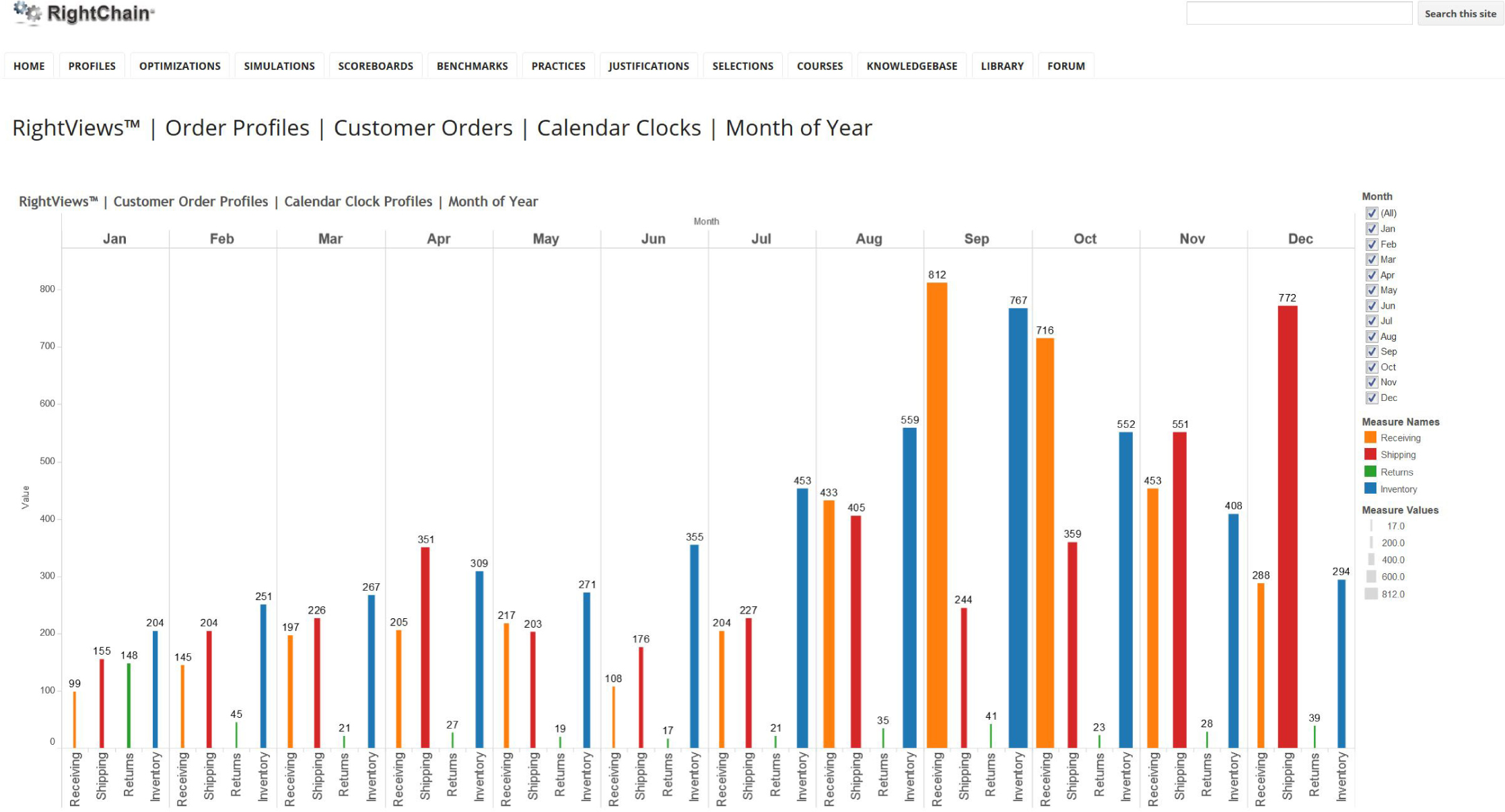
The seasonality profile indicates the peaks and valleys in inventory levels, as well as receiving, shipping, and returns activity. Because storage systems need to be sized to accommodate near-peak inventory levels and material-handling systems need to be sized to accommodate near-peak activity levels, it is critical to identify peak inventory and activity levels. The example is typical of retail distribution, with receipts peaking in August/September, inventory peaking in September/October, shipping peaking in October/November, and returns peaking in January. A distribution presents an opportunity to shift the extra staff required for receiving in August/September to shipping in October/November to returns handling in January.
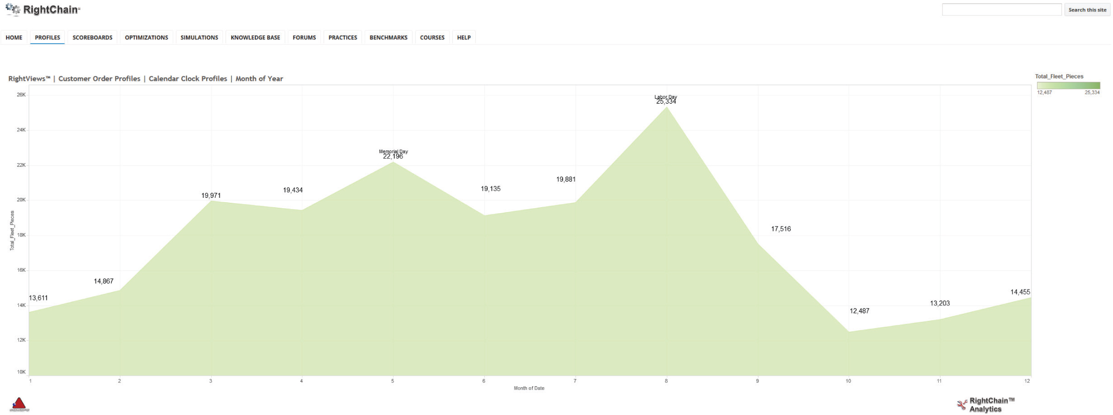
One of our furniture clients experiences the same volatility but in different seasons (Figure 2.21). As we learned from our work with them, summer is their busiest season based upon their major sales during the Memorial Day and Labor Day holidays.
Figure 2.21 Seasonality distribution for a large furniture company.
Week-of-Month Activity Distribution
Most shipping activity occurs during the last week of the month, especially during the last month of a quarter (Figure 2.22). Conversely, most receiving activity occurs during the first week of the month, especially during the first month of a quarter.
Figure 2.22 Week-of-month activity profile.

Day-of-Week Activity Distribution
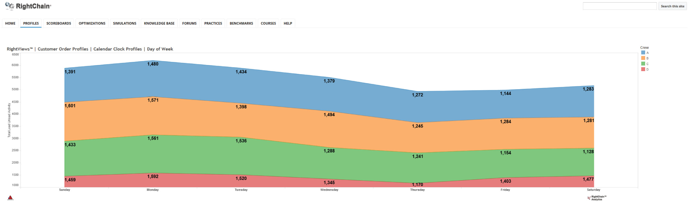
The day of the week is another driving force in many warehouse activity peaks and valleys. We recently completed a supply chain strategy project for one of the world’s largest bedding manufacturers (Figure 2.23). Most of the mattresses purchased in the world are purchased on Saturday, with deliveries scheduled for the following Friday. Needless to say, Thursday and Friday are very busy days in their warehouses.
Figure 2.23 Day-of-Week activity profile for a large bedding company.

In recent project in the food and beverage industry, two retailers comprised nearly 50 percent of their outbound volume. Unfortunately, each wanted deliveries executed on the same two days of each week. Needless to say, the two days before were overwhelming peaks for the warehouse operations (Figure 2.24).
Figure 2.24 Day-of-Week activity profile for a food and beverage company
Hour of Day Activity Distribution
As the name suggests, the Hour-of-Day profile indicates (Figure 2.25) the receiving, putaway, picking, and shipping activity by hour of the day. Material handling systems should be designed for peak activity periods. Offsetting peaks represent opportunities for shift staggering and inter-department workforce shifting.
Figure 2.25 Hour-of-Day distribution for dock door receiving activity.

2.4 Item Activity Profiling
The item activity profile is used primarily to slot the warehouse, to decide for each item (1) what storage mode the item should be assigned to, (2) how much space the item should be allocated in the storage mode, and (3) where in the storage mode the item should be located. The item activity profile includes the following activity profiles:
![]() Popularity profile
Popularity profile
![]() Cube–movement profile
Cube–movement profile
![]() Popularity-cube–movement profile
Popularity-cube–movement profile
![]() Order-completion profile
Order-completion profile
![]() Demand-correlation profile
Demand-correlation profile
![]() Demand-variability profile
Demand-variability profile
Item Popularity Profile
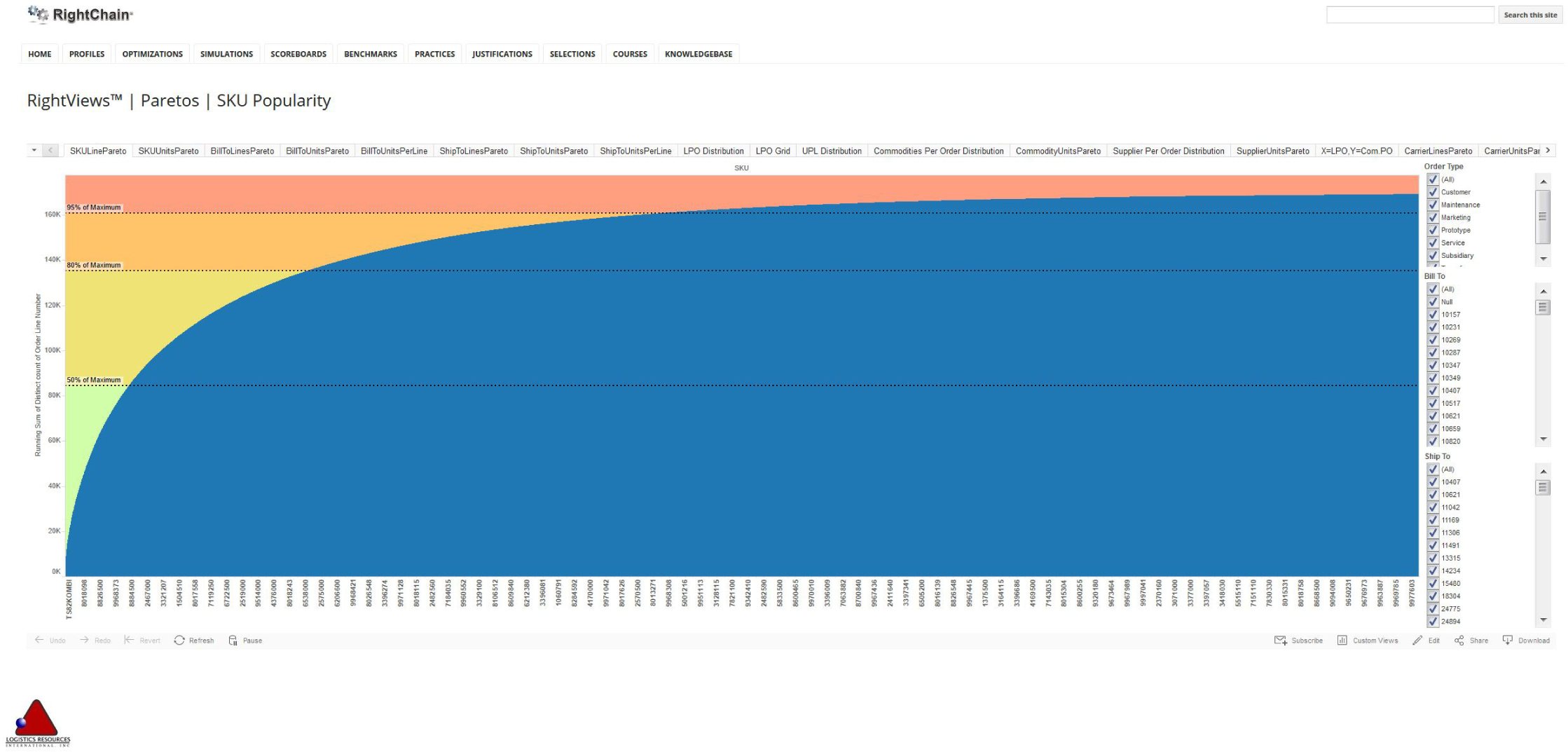
As mentioned earlier, a minority of the items in a warehouse typically generates a majority of the picking activity. The popularity profile (sometimes called an ABC curve or a Pareto distribution) indicates the x percent of picks associated with y percent of the SKUs (ranked by descending popularity). Figure 2.26 is a classic popularity profile indicating that the 10 percent most popular items yield 70 percent of the picking activity, the 50 percent most popular items yield 90 percent of the picking activity, and so on. Key breakpoints in the distribution suggest delineations between item popularity families. For example, the top 5 percent of items (Family A) may make up 50 percent of the picking activity, the next 15 percent of items (Family B) may take us to 80 percent of the picking activity, and the remaining 80 percent of items (Family C) cover the remaining picking activity. These families, in turn, may suggest three alternative storage modes—Family A in an automated, highly productive storage mode; Family B in a semi-automated, moderately productive picking mode; and Family C in a manual picking mode that offers high storage density. The family breakpoints also may suggest the location of the items within a storage mode—A items located in the golden zone (close to a travel aisle and/or at or near waist level), B items in the silver zone, and C items in the remaining spaces. The overriding principle is to assign the most popular items to the most accessible warehouse locations.
Figure 2.26 Item popularity profile for a large service parts company.
Cube-Movement Profile
The cube-movement profile is used primarily for making storage-mode and space-allocation decisions. The cube-movement profile indicates the portion of items that falls into pre-specified cube-movement ranges. If the pre-specified ranges correspond to storage-mode alternatives, then the cube-movement profile will essentially solve the storage-mode assignment problem. For example, in Figure 2.27, 15 percent of the items ship less than 0.1 cubic feet per month. Those items may be good candidates for storage drawers or bin shelving. At the other end of the distribution, we find 12 percent of the items that move more than 1,000 cubic feet (nearly 20 pallets) per month. Those items may be candidates for block stacking, double-deep rack, push-back rack, and/or pallet flow lanes.
Figure 2.27 Cube-movement profile for a large valves and fittings company.
Popularity–Cube-Movement Profile
Done properly, slotting takes into account both the item popularity and cube-movement. An example popularity–cube-movement profile for broken-case picking is presented in Figure 2.28.
Figure 2.28 Popularity–Cube-Movement Profile
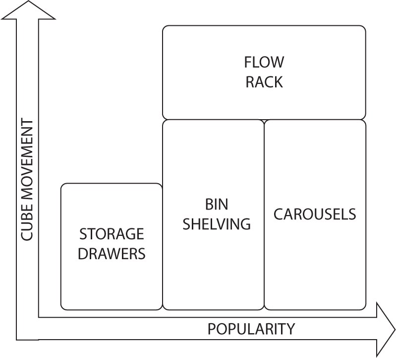
In this example, those items exceeding a certain cube-movement threshold are assigned to a carton flow rack. Items with high cube-movement need to be restocked frequently and need a larger storage location compared to items with medium and low cube movement. Hence they need to be assigned to a storage mode that facilitates restocking and condenses large storage locations along the pick line–carton flow rack. Items with low cube movement and high popularity generate many picks per unit of space that they occupy and do not occupy much space along the pick line. They need to be in a highly productive picking mode. In this case, light directed carousels are recommended because the picking productivity is high, and we can afford the carousels for items that do not need large storage housings on the pick line and do not need to be restocked frequently. (Carousels do not lend themselves to restocking and are expensive per cubic foot of space.)
Items with low popularity and low cube movement cannot be justifiably housed in an expensive storage mode. Hence they are candidates for bin shelving and modular storage drawers.
Items in the bottom right-hand quadrant of each preference region generate the most picking activity per unit of space they occupy in the storage mode. Hence they should be assigned to positions in the golden zone (most accessible pick locations) of their storage mode. Items in the upper right-hand and lower left-hand quadrants generate a moderate number of picks per unit of space they occupy in the storage mode. Hence they should be assigned to positions in the silver zone. Finally, items in the upper left-hand quadrant of the distribution generate the fewest picks per unit of space they occupy and they should be assigned positions in the bronze (least accessible) zone.
This example is not an end-all recommendation for slotting broken-case picking systems. This depends on many other factors, including the wage rate, the cost of space, the cost of capital, the planning horizon, and so on. Instead, this example is presented to illustrate how the popularity–cube-movement distribution is used in slotting.
Item-Order-Completion Profile
The item-order-completion profile (Figure 2.29) identifies small groups of items that can fill large groups of orders. Those small groups of items often can be assigned to small order-completion zones in which the productivity, processing rate, and processing quality are two to five times better than those found in the general warehouse.
Figure 2.29 Item-order-completion profile.
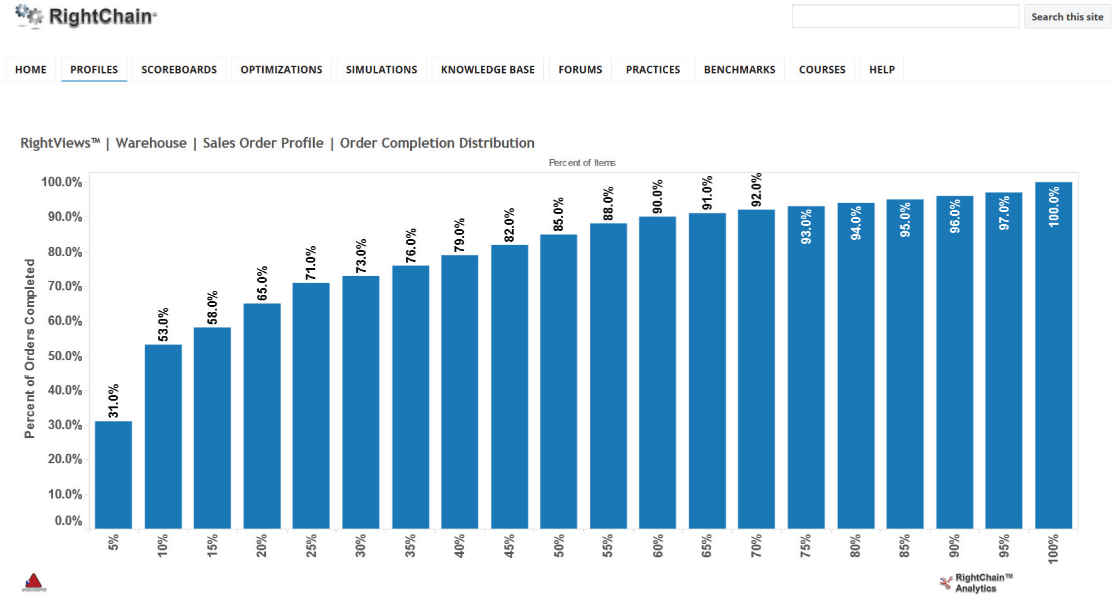
The item-order-completion profile is constructed by ranking items from most to least popular. Beginning with the most popular item, then the two most popular items, then the three most popular items, and so on, the items are compared with the order pool to determine what portion of the orders a given subset of the items can complete. In this example, 10 percent of the items can complete 50 percent of the orders. Suppose that I walk into your warehouse and identify 10 percent of the items that can completely fill 50 percent of the orders. What would you do with those 10 percent of the items? I hope that you would create a warehouse within the warehouse or order-completion zone for those 10 percent.
The design principle is similar to that used in agile manufacturing, where we look for small groups of parts that have similar machine routings. Those machines and those parts make up a small-group technology cell wherein the manufacturing efficiency, quality, and cycle time are dramatically improved over those found in the factory as a whole.
We recently worked with a large media (i.e., compact discs, cassettes, videos, etc.) distributor and helped to identify 5 percent of its 4,000 SKUs that could complete 35 percent of its orders. We assigned those 5 percent to carton flow-rack pods (three flow-rack bays per pod, one operator per pod) at the front of the distribution center. Operators could pick/pack orders from the flow rack at nearly six times the overall rate of the distribution center. The distribution center has won its industry’s productivity award each of the last two years.
Very frequently, there is a driving force behind order completion. Examples could include customers ordering within a brand (Figure 2.30) or, as depicted in Figure 2.31, a product group, a supplier, a size, a color, a kit, and so on. Our pattern-recognition algorithms seek and surface those patterns in an attempt to identify order-completion zoning opportunities within the warehouse.
Figure 2.30 Item-order-completion profile from a large food and beverage company.
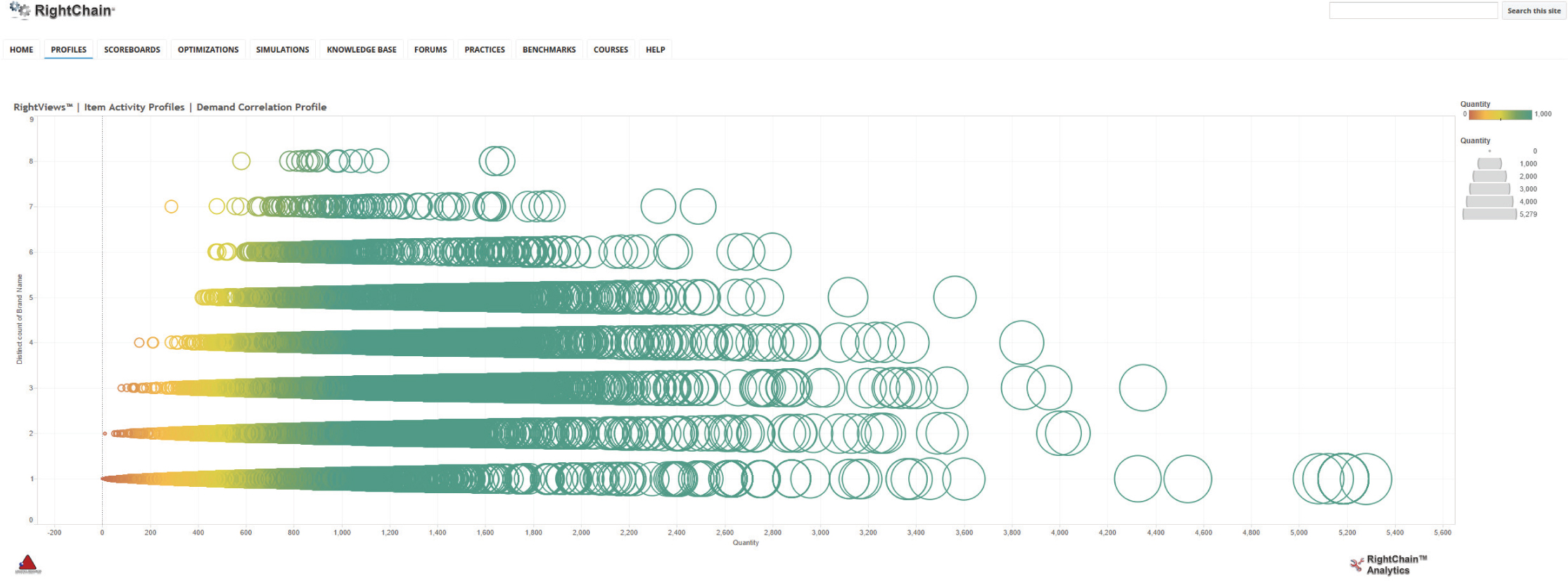
Figure 2.31 Order-completion profile for a large industrial supplies company.

Demand-Correlation Profile
Just as a minority of the items in a warehouse makes up a majority of the picking activity, certain items in the warehouse tend to be requested together. In the example (Figure 2.32), pairs of items are ranked based on their frequency of appearing together on orders. In this case, we are examining data from a mail-order apparel company. The first three digits represent the style of the item (i.e., crew-neck sweater, V-neck sweater, turtle-neck shirt, pleated pants, etc.), the middle digit represents the size of the item (i.e., 1 = small, 2 = medium, 3 = large, and 4 = extra large), and the last digit represents the color (i.e., 1 = white, 2 = black, 3 = red, 4 = blue, 5 = green, etc.).
Figure 2.32 Demand-correlation distribution (style-size-color) for a large omni-channel retailer.
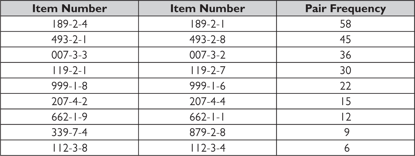
What do you think people tend to order together from this mail-order company? (I thought it would be shirts and pants that looked good together in the catalog.) What does the profile in Figure 2.32 suggest? In this case, customers tend to order items of the same style and size together. The explanation is that customers tend to get comfortable with a certain style and tend to order in multiple colors to add variety to their wardrobes. Of course, they order the same size unless they will return one for fitting. This pattern was a surprise to me. It was also a surprise to the marketing people. Surfacing truth is the crucial benefits of profiling process. (The myriad SKUs, order patterns, suppliers, and interdependent decisions make it difficult to form a reliable intuition about logistics operations.)
How do we take advantage of this demand-correlation information in slotting a warehouse? We zone the warehouse by item size first, creating a zone for the smalls, mediums, larges, and extra larges of all styles (Figure 2.33). Within each size area, we store items of the same style together, mixing colors within a style. This zoning strategy allows us to create picking tours based on size and style. As a result, order pickers pick many items on short-distance picking tours. Simultaneously, we manage congestion by spreading out the sizes. Golden zoning is used to slot the most popular color for each style at or near waist level.
Figure 2.33 Slotting optimization for a large omni-channel apparel retailer.

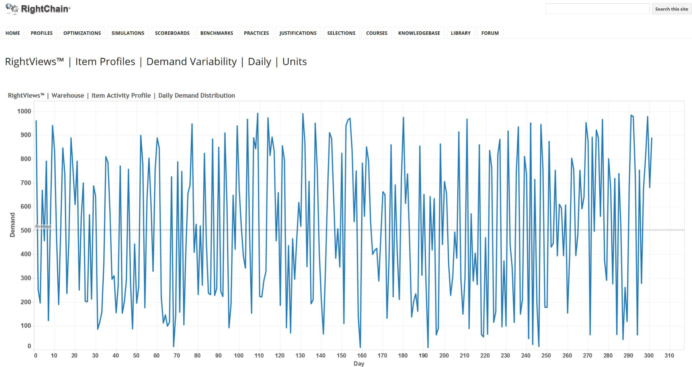
Demand-Variability Profile
The demand-variability profile (Figure 2.34) indicates the standard deviation of daily demand for each item. Unfortunately, an item’s daily demand is not predictable. During a recent project, we were trying to size the pick faces along a case picking line such that each pick face held a day’s worth of stock. The motivation was to make sure that we did not need to restock a location during the day. The current design had the pick faces sized for an average day’s demand, and the client could not figure out why it had to restock so many locations during the course of a day. You can probably see why. If the pick face is sized for the average day, unless the same quantity is picked every single day, there will be many days when the pick face is oversized and many days when the pick face is undersized. Once the pick faces were resized to accommodate this variability in demand, the restocking during the pick shift was virtually eliminated.
Figure 2.34 Demand-variability profile for a large textile company.
2.5 Inventory Profile
The inventory profile includes the item-family inventory profile used to reveal opportunities for improved inventory management practices and the handling-unit inventory profile used in storage systems planning.
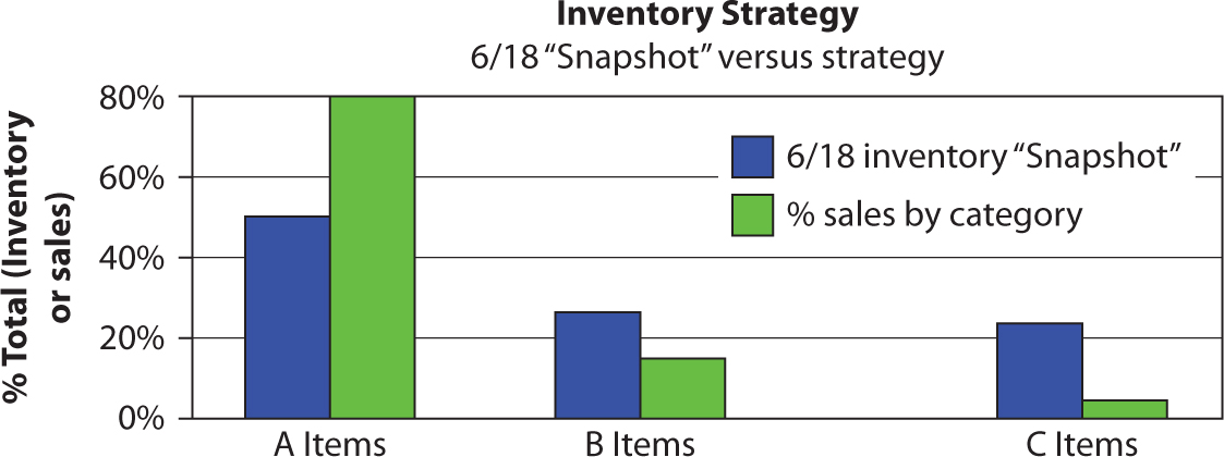
On-Hand Inventory Profile
I receive a lot of phone calls that begin with clients complaining about the lack of space in their warehouse. More often than not, the problem is not too little space, but too much inventory. This profile (Figure 2.35) helps us identify the source of the inventory problem. As is true in the example, most companies have too little type A inventory (back orders and customers screaming for those products) and too much type C inventory (obsolete stock that nobody wants and nobody has the courage to discard). By drawing the picture, we can at least illustrate the magnitude of the problem to management and present a list of “problem items” for their review.
Figure 2.35 Item-family inventory distribution.
In some cases, C items should be removed from inventory. However, in many cases, warehouses are required to house the C items. One example is in the service parts business, where you may be required to support a certain model number in the field for up to 5, 10, even 20 years. Another example is in retailing when some key type C items protect the sales of items A and B. On a recent project in the grocery industry, the chairman of the company was presented with a recommendation to eliminate the C items from inventory. Let’s pause and consider the consequences. How many items do you buy on your weekly trip to the grocery store to restock the kitchen cabinets? Say its 50 items. In this case, there is at least a 70 percent chance that one of those 50 items is a C item. Why did you go to that grocery store? In the case of this grocery chain, it was probably because it stocked that C item. Otherwise, you could and would shop at a warehouse store.
Even though you may not be able to eliminate the C item inventory you can at least efficiently store and pick the items. To conserve space, you can store the C item inventory in dense, high-rise racking or on the second or third level of a mezzanine. To achieve high productivity at the same time, you can batch-pick the C item pick line and locate the batch in a dedicated location along the forward pick line or introduce the batch into an automated sorting system.
Handling Unit Inventory Profile
The item-family inventory profile is not very useful for storage systems design because the information is not presented in material-handling terms (i.e., pallets, cases, eaches, etc.). This is a common problem with most corporate data used in planning warehouse operations—the data are expressed in terms of dollars, pounds, pieces, days of supply, turns, and so on. Although this is useful for business planning purposes, the data are not very helpful for planning and managing warehouse operations. This is another motivation for the profiling exercise—to give managers and designers of the warehouse operations a presentation of the activity of the warehouse in their terminology.
In this example (Figure 2.36), we convert the item-family inventory distribution into a distribution describing on-hand inventory in terms of pallets of merchandise on hand. As a result, we can recommend the appropriate mix of pallet storage modes. For example, the 91 SKUs with less than a pallet of inventory on hand probably should be stored in shelving or decked racking. The 104 SKUs that have one or two pallets on hand probably should be stored in single-deep pallet racks. The 68 SKUs that have three to five pallets on hand probably should be stored in double-deep and/or push-back racks. The remaining SKUs, those with more than 10 pallets on hand, probably should be stored on the floor in deep block stacking lanes, in drive-in/through racks, and/or in pallet flow lanes.
Figure 2.36 Handling-unit inventory distribution for a large healthcare company.
