
Pattern Feature Extraction
In Chapter 1 we said that the basis of pattern recognition is the ability to transform a pattern function into another representation. In particular, extracting features from a pattern function can be regarded as generating different representations of the pattern.
In this chapter we will discuss various methods for extracting features from a pattern function and various methods for representing the extracted features. The patterns we consider here are visual patterns. The features of a visual pattern provide the macro information that enables us to distinguish one pattern from another. For example, edges for distinguishing light and shadow, boundary lines or surfaces of an object included in the pattern or the region surrounded by such lines or surfaces, the texture of a surface, and the direction of movement are typical features in a visual pattern. There are many methods of representing these features. In this chapter we will describe algorithms for extracting some of these features and methods of representing the extracted features.
4.1 Detecting an Edge
First we describe a method for detecting an edge in a visual pattern. The edge of an object is a local boundary that distinguishes the surface of the object from other objects or surfaces. The reason we say local is that we use the word edge to mean a part of the boundary rather than the whole boundary line or surface. The edge of an object generally corresponds to a part of the pattern where the value of the pattern function changes drastically. Therefore, in order to detect an edge, we first need to compute the spatial change in the value of a pattern function.
Below we describe the zero-crossing method using second-order differentials and the difference operator method using first-order differences. Both are popular methods for finding spatial change in the intensity values of pattern functions.
(a) The zero-crossing method
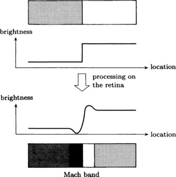
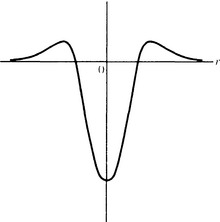
In the visual recognition systems of some organisms, there is a mechanism called the Mach band. This mechanism, as shown in Figure 4.1, makes contrast more pronounced by automatically computing the differential of the intensity of light across the edge of an object that abruptly changes brightness when projected on the retina. By formalizing this mechanism, we obtain a method where, in a pattern function that represents the intensity of light, we find the points that make the second-order differential of the function equal to 0, generate a line combining these points, and use this line as an edge of an object. This is called the zero-crossing method. We explain the zero-crossing method in detail below.
Let f(x, y) be a pattern function in two-dimensional Euclidean space. Since a pattern function like f(x, y) usually includes noise, we first remove the noise by applying some method of smoothing. For example, by taking a local weighted average of the original values of a pattern function as the value at some pattern element, the values of a pattern function at neighboring pattern elements change smoothly. In this way we can hope to remove noise in a pattern function and recreate the original data. By using the Gaussian operator
as a smoothing function, the value of the pattern function after smoothing, g(x, y), is
The second-order differential of g(x, y) is found by applying g(x, y) to the two-dimensional Laplacian operator
Thus, the second-order differential of g(x, y) is
where
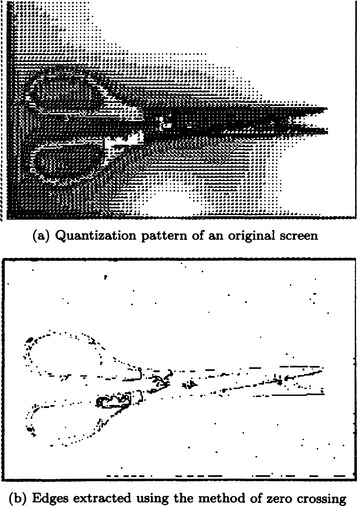
A point where k(x, y) = 0 is called a zero crossing. By connecting zero crossings, we can obtain an edge. Figure 4.2 shows a section of ∇2 H(r). Figure 4.3 shows an example of edges extracted using the method of zero crossings.
(b) The difference operator method
We now describe the use of the method of first-order differences as applied to pattern functions. It is possible to formalize this using first-order differentials, but, since our goal is to find an edge using a computer, we think it is more practical to formulate it using differences.
First, we assume that a given pattern function represents the intensity distribution of the image. In order to make it simple, we also assume that we know the direction of the change in intensity. If we let the x axis be the direction of the change of intensity and let the intensity at the point x be f(x), the difference of the intensity at x is
where k is the length of the difference interval. Now, in order to remove noise, we can do smoothing by averaging over k. For example,
For usual applications, values around k1 = 1, k2 = 2-5 are used. The advantage of the above formula is that f(x+i) and f(x-i) can be computed directly using data from the pattern function.
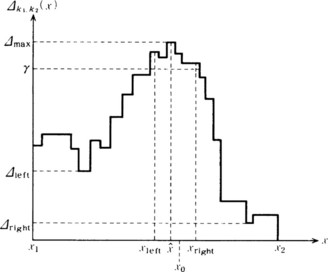
We compute Δk1,k2(x) in some interval, [x1,x2], and then estimate the location of an edge. Although the location of an edge should be at a point ![]() where the difference, Δk1,k2(x) takes a maximum in [x1, x2], we usually use the following algorithm, which takes the interference of noise into account.
where the difference, Δk1,k2(x) takes a maximum in [x1, x2], we usually use the following algorithm, which takes the interference of noise into account.
Algorithm 4.1 (estimating the location of an edge)
[1] Estimate the existence of an edge using the following substeps. If the system succeeds in estimating the existence of an edge, go to [2]. Otherwise, stop.
[1.1] Find the maximum value of Δk1,k2(x) on the interval [x1,x2]. Call this value Δmax and let ![]() be one of the points that take
be one of the points that take ![]() .
.
[1.2] Let Δleft and Δright be the minimum values of Δk1,k2(x) on the intervals ![]() and
and ![]() , respectively.
, respectively.
[1.3] If the following is true for some given threshold values α1 and α2. assume that an edege exists near ![]() :
:
[2] Estimate the location of an edge using the following substeps:
[2.1] For given parameters β1 and β2 ((β1 > 0), set
[2.2] Among points to the left of ![]() on the x axis, let xleft be the leftmost point such that Δk1,k2(x) ≥ γ is true for each point between such a point and
on the x axis, let xleft be the leftmost point such that Δk1,k2(x) ≥ γ is true for each point between such a point and ![]() In other words,
In other words,
[2.3] Among points to the right of ![]() on the x axis, let xright be the rightmost point such that Δk1,k2(x) ≥ γ is true for each point between such a point and
on the x axis, let xright be the rightmost point such that Δk1,k2(x) ≥ γ is true for each point between such a point and ![]() In other words,
In other words,
[2.4] Estimate the location of the edge, xo, as the midpoint between xieft and xright. In other words,
Figure 4.4 shows an example of estimating the location of an edge using the above algorithm.
(c) Estimating the direction of intensity change
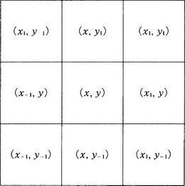
In method (b) we assumed that the direction of the edge was orthogonal to the x axis. If the direction of the edge is unknown, this method is useless. In this case, we need to find the direction of the intensity change, in other words, the direction that meets the edge at a right angle. We now describe a method for finding this direction. Consider the 3×3 window with some point (x, y), in two-dimensional Euclidean space E2, as its center, as shown in Figure 4.5. The (difference) gradient of light at (x, y)
is obtained using the following formulas:
Furthermore, the direction of the gradient vector at (x, y), v, can be obtained from
We can use v(x, y) as the direction of the x axis in (b). In that case, the direction of the edge is v + α/2 at the point (x, y). Also, the magnitude of the gradient, in other words, the change of intensity at (x, y), is
In the above example, we used a 3 × 3 window; however, we can use a bigger window, for example, 5×5. In this case, the formulas for the gradient will be slightly different.
4.2 Detection of a Boundary Line
In the recognition of visual patterns, it is important to detect boundary lines that distinguish an object from its background, or two surfaces of an object. Detection of a boundary is usually done by somehow grouping many small edges discovered using the methods described in Section 4.1. Constructing a line segment or curve by grouping local edges is called segmentation. In this section we explain the edge tracing method, the edge prediction method, and the Hough transformation method, all of which are popular methods for detecting boundary lines.
(a) Edge tracing
Once we have found the direction of the gradient of each edge from a visual pattern function, we can detect a boundary line by tracing the edge in the direction orthogonal to the gradient. This method is called the edge tracing method. The edge tracing method traces an edge using heuristic search on a graph that is constructed using the directions of gradients. What to use as an evaluation function for the heuristic search depends on what kind of boundary lines we are looking for. For example, by using shortest-path search, a boundary line is determined by a group of the shortest lines. Evaluation functions including the magnitude of the gradient or curvature (which can be obtained from the difference in the direction of neighboring gradients) can also be used.
As an example, let us suppose that we have found the direction orthogonal to the gradient at each point as shown in Figure 4.6(a). Let us imagine the graph G shown in Figure 4.6(b), which takes each point with the direction of the gradient at that point as its nodes and has a directed edge in that direction. We assume that, of the three neighboring nodes that are within ± 90 degrees of the orthogonal direction, ρ, of the gradient at a node, ui of G, only the nodes that are closer than ±90 degrees from ρ are direct destinations of edges from ui. For example, in G, the node u1 has an edge to u2, u3, and u4, respectively. Also, the node u2 has an edge to u5 and u6. However, there is no edge from the node u5 to u6.
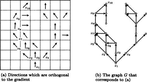
Next, let us assume that the end points ui and uj of the boundary line are already known. Now, if we search for the shortest path from the end point ui to uj on the graph, we will be able to construct the boundary line we are looking for as a set of segments. For example, in the graph G in Figure 4.6(b), one of the shortest routes from u1 to u10 is the path passing through u1, u2, u5, u7, u8, u9, and u10. We can use edges on this path as a representation of the boundary line.
Below, we will show the basic algorithm for the edge tracing method.
Algorithm 4.2 (edge tracing)
[1] Using the method described in Section 4.1, compute the direction of the gradient
and the magnitude of the gradient
for each point (x, y) in the domain of the pattern function. Assume ![]()
[2] Define the graph G = (U, L) as follows:
(i) Make each point (x, y) for which we have computed ρ(x, y) correspond to a node of G.
(ii) Let ui and uj be the nodes that correspond to two neighboring points, (xi,yi) and (xj,yj). Assume that a directed edge from ui to uj exists if and only if (xj,yj) is one of the three neighboring points in the ρ(xi,yj) direction from (xi,yi) and when all of the following inequalities hold:
where k is a given positive constant.
[3] Pick two nodes of G, uo and ud, and let uo be the initial state so and ud be the goal state sd. Do the shortest-path search from so to Sd using the best-first search described in Section 3.6. For the shortest-path search, we use an evaluation function whose value at a node is the length of the path followed so far.
Formula (1) in condition (ii) of [2] above is a heuristic rule to make the orthogonal direction of the gradient closer to ud. Formulas (2) and (3) are heuristic rules for recognizing only gradients of a certain magnitude as contributing to the boundary line, in order to prevent confusion between an edge and noise.
(b) Edge prediction
In this section we describe the edge prediction method, a boundary detection method similar to the edge tracing method. Intuitively the edge prediction method starts from an edge, predicts the direction of a neighboring edge, and combines edges based on that prediction. The basic algorithm is shown below. The algorithm for this method is simple, and it is possible to use it along with other edge detection methods. Also, it is, in principle, possible to generate not only line segments but also curves. However, since this method computes serially using local data from the pattern function, it may find different boundaries depending on what we take as the initial edge. It is also easily affected by noise.
Since the following algorithm is conceptual, to turn it into a program, we would need to supply programs for edge detection or extrapolation of line (or curve) segments.
Algorithm 4.3 (edge prediction)
[1] Pick one edge and assume that it is the currently considered edge. Assume no boundary lines have been obtained so far. Let the current edge be the initial boundary line. (Selection of the initial edge)
[2] Extend the boundary obtained so far along the current edge and predict the location of the end of the extension and its direction. The direction of the extension is generally not unique but is usually distributed over some area. (Prediction of the neighboring edge)
[3] Find a neighboring edge within the area predicted in [2] using some edge detection method. If a neighboring edge was found as predicted, add it to the boundary and go to [2]. If an edge was detected outside the predicted area, go to [4]. If an edge could not be found, go to [5]. (Detection of a neighboring edge)
[4] Assume that one boundary line ends at the current edge and stop the algorithm. (Termination of prediction)
[5] If an edge could not be found persistently for several trials, decide that the boundary ends at the current edge and stop the prediction.
Otherwise, decide that the reason for not being able to find the edge is the effect of noise, go to [2], and predict another direction. (Decision to continue prediction)
(c) Hough transformations
Fitting a curve to many local edges can be done by finding a formula for a curve that passes through as many points as possible that make the magnitude of the gradient larger than a certain value. One method for detecting a boundary line by making use of this idea is called the Hough transformation method. The Hough transformation works particularly well when many edges have been obtained. Compared with the edge tracing method and the edge prediction method, it is less likely to be affected by noise. Let us consider the Hough transformation method here.
As an example, suppose we fit a straight line to a set of edges generated from a pattern function in two-dimensional Euclidean space. Let {p1,…, pn}{pj = (xj,yj),j = 1,…, n) be points where the magnitude of the gradient goes over a given threshold. If the straight line ![]() passes through the points p1,…, pk1 ≤ k ≤ n), then
passes through the points p1,…, pk1 ≤ k ≤ n), then ![]() holds. This means that, if we map these functions into the space of the parameters (a, b), there are k straight lines b = −xja+yj (j = 1,…, k) that intersect at one point,
holds. This means that, if we map these functions into the space of the parameters (a, b), there are k straight lines b = −xja+yj (j = 1,…, k) that intersect at one point, ![]() . That is, grouping the original n points, P1 … Pn and putting the points of each group on a straight line is equivalent to finding the intersection point of straight lines in the space of the parameters, (a, b).
. That is, grouping the original n points, P1 … Pn and putting the points of each group on a straight line is equivalent to finding the intersection point of straight lines in the space of the parameters, (a, b).
Suppose, as shown in Figure 4.7(a), we have the points, {P1,…, P5} = {(2,2), (2,3), (4,4), (5,5), (6,5)}. In this case, the straight lines that correspond to p1}i,…, p5} in the parameter space will be the following:
(see Figure 4.7(b)). The number of points of intersection of these five straight lines is five, A, …,E, as shown in Figure 4.7(b). Each point corresponds to the straight line that combines the points in Figure 4.7(a). We assume here that the points p1 and p2 have the same x coordinate and that the straight lines corresponding to p1 and p2 are parallel in the parameter space, since the slope of the straight line a, which combines p1 and p2, is infinite.
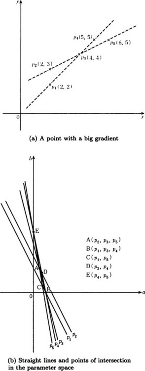
As you can see from this example, in general, the number of straight lines that intersect at a point is different for each point of the intersection in the parameter space. Usually, when you use this method for detecting a boundary, it is desirable to choose, as a boundary line, a straight line that passes through as many points as possible in the original space, or equivalently a point of intersection where as many lines as possible intersect in the parameter space (called the maximal intersection). In the above example, points A and B in Figure 4.7(b) are the points with maximumal intersection. The straight lines that correspond to A and B in the original space are the two broken straight lines shown in Figure 4.7(a). These two straight lines segment the edges.
The method above can be used not only for straight lines but also for simple curves. The method of detecting a boundary line by transforming the original problem to one of computing points of intersection in a parameter space is called the Hough transformation method. An algorithm for the Hough transformation for finding a straight line that passes through as many as points as possible can be summarized as follows:
Algorithm 4.4 (Hough transformation for fitting a straight line)
[1] Quantize the parameter space between the maximum values and the minimum values that a and b can take. Call the quantized parameters a1,…, ar, b1,…, bs. (Quantization of the parameter space)
[2] Make aj = 0 (j = 1,…, r), bk = 0 (k = 1,…, s). (Initialization of parameters)
[3] For each point pi = (xi, yi) whose gradient magnitude exceeds a certain threshold value, let
for aj, bk such that ![]() . (Detection of an intersection point in the parameter space)
. (Detection of an intersection point in the parameter space)
[4] Find a point (a, b) that takes a maximal value in the quantized parameter space. This (a, b) corresponds to a set of points that have large gradients and are all on one straight line. (Detection of a straight line)
However, as we noted in the previous example, this algorithm cannot find a straight line passing through two points whose x coordinates are the same in the original space, in other words, a straight line passing through two points arranged vertically. Thus we often use the above method with a polar coordinate space as the parameter space and transform a point (x, y)to a sine wave in the space of parameters (r, θ) by using x cos θ + y sin θ = r. The Hough transformation method is often used as a boundary detection method for cases with many local edges or with noise.
4.3 Extracting a Region
Once boundary lines have been detected, we can use this line to extract the region surrounded by the boundary lines. In this section we will describe two popular algorithms for extracting a region, the splitting method and the merging method. Before we do that, we need to define the word “region.” A region is a set of pattern elements defined as follows:
Definition 1
(partition and region) Let D be a finite set of pattern elements from a given pattern function and let 2D be the set of subsets of D. Let Q(D) be a predicate on 2D that, for any subset of pattern elements, D ∈ 2D, returns T if the elements in the subset have uniform values and returns T returns F otherwise. A set of pattern element sets D1,…, Dn is called a partition of I for a predicate Q if
and
Each pattern element set, Di (i = 1,…,n), of the partition is called a region.
(a) Splitting method
As noted in Definition 1, in order to determine a region, we need a predicate for judging whether the pattern elements included in that region have uniform values or not. Let us consider the following predicate Q as an example:
where f(x) is a pattern function and c is a given constant.
For this predicate Q, we are only considering a pattern element set D where either all x ∈ D make f(x) > c or all x ∈ D make f(x) ≤ c. Therefore, Q is a predicate applicable only when the value of a pattern function distinguishes an object from its background. In other words, if we let D1 and D2 be the sets of pattern elements for an object and its background, respectively, then Q is a predicate for extracting D1 and D2 so that Q(D1) = T and Q(D2) = F.
Region extraction of this kind can be done approximately by setting an appropriate threshold value c. For example, if we make a histogram for the values of a pattern element, f(x), and remove small variations of values by smoothing it, then we can use the minimal value as the value of c. We can smooth a histogram, for example, using the method of fitting the histogram to the sum of two normal distributions and determining the threshold value from the estimated parameter values.
The above method of region extraction is generally called the splitting method. This method can extract smaller regions by using the same method of splitting recursively. An algorithm for such a recursive splitting method is as follows:
Algorithm 4.5 (region extraction using the recursive splitting method)
[1] Let the domain, D, of a given pattern function, f(x), be the initial region. Set D = {D}. (Definition of the initial region)
[2] Construct the histogram of the values of f(x) on the pattern elements. (Construction of the histogram)
[3] Smooth the histogram and determine the threshold value as the minimal value in the histogram. (Finding the threshold value)
[4] If there is no minimal value in the histogram, stop. D is the extracted region. Otherwise, go to [5] using c as the threshold value. (Termination condition)
[5] Let D1 {x|f(x) > c} and D2 = {x|f(x) ≤ c}. Let D = D ∪ {D1,D2} − {D}. (Extracting a region)
The splitting method is a global method for extracting regions based on the whole distribution of intensity values of a pattern function and is robust against noise. We can also search for threshold values by constructing a multidimensional histogram using, for example, intensity and some other attributes like color. It is sometimes even easier to find threshold values if we use a multidimensional histogram.
(b) Merging
While the splitting method uses global data, the merging method uses local data. The merging method first considers a small set of pattern elements as one region. As the smallest set, it can take each pattern element. It then merges neighboring regions when the difference between the average values of the pattern function in those regions is smaller than some given threshold value. By repeating this operation, we can extract a larger region with uniform values of the pattern function. Depending on how we define the average value of a region, many methods are possible. We will provide one of them below.
Algorithm 4.6 (region extraction by merging using the difference in values of the pattern function on two sides of a boundary line)
[1] Detect boundary lines by applying some boundary detection algorithm to a given pattern function.
[2] Do the following substeps for all boundary lines, k:
[2.1] Assume that the sets of pattern elements found on the two sides of the boundary line k are regions ak and bk, respectively.
[2.2] Let Lk be the length of k. Let Mk be the sum of the lengths of the parts of k for which differences in values of the pattern elements in ak and bk are smaller than a given value.
[2.3] For a given threshold value, c, merge ak and bk, and delete k only when Mk/Lk < c.
[3] If the merge does not happen for any of the current boundary lines in [2], then stop. Otherwise, go to [2].
There is also a method, called the split-and-merge method, that combines the splitting method and the merging method.
4.4 Texture Analysis
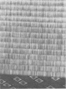
There are visual patterns that can be considered as single patterns at the level of a region, though local features such as directions of edges and differences of intensity are similar in each of those patterns. For example, Figure 4.8, part of a tatamimat, produces a pattern by repeating similar elements. A pattern like this, which is created by repeating elements with some invariant feature, is called a texture. An element constituting texture is called a texture primitive or a texel.
To consider texture as one feature of the surface of an object and extract such a feature from the pattern function corresponding to the object is called texture analysis. In this section, we will explain some methods of texture analysis.
(a) Structure analysis
Considering the fact that a texture usually is generated by repeating elements that are similar in shape but are placed slightly differently, we can do texture analysis based on a kind of grammar whose elements are shapes. For example, let us consider the texture shown in Figure 4.9(a). This texture is generated by iterating ![]() and
and ![]() . In order to generate such a texture, we can use the grammar, {S, C, R, S0}, shown in Figure 4.9(b), where S, C, R, and S0 represent the set of terminal symbols, the set of nonterminal symbols, the set of grammar rules, and the initial symbol, respectively. (S0 is equivalent to a sentence in a linguistic grammar.)
. In order to generate such a texture, we can use the grammar, {S, C, R, S0}, shown in Figure 4.9(b), where S, C, R, and S0 represent the set of terminal symbols, the set of nonterminal symbols, the set of grammar rules, and the initial symbol, respectively. (S0 is equivalent to a sentence in a linguistic grammar.)
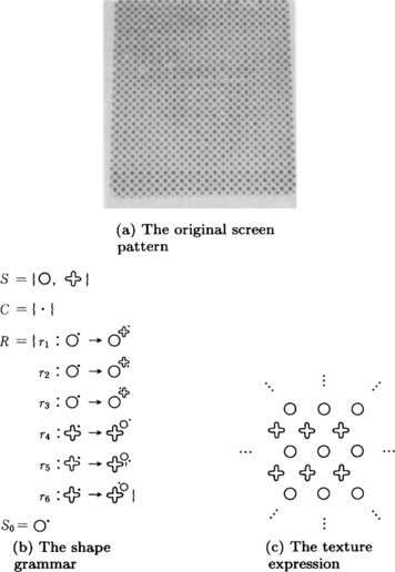
By starting from the initial symbol, S0, and applying one of the grammar rules, r1 − r6, we can generate the texture shown in Figure 4.9(c). (In the rules, ![]() ,
, ![]() ,
, ![]() , and
, and ![]() and
and ![]() , and
, and ![]() are identified, respectively.) A grammar like the one shown in Figure 4.9(b) is called a shape grammar. In order to apply a shape grammar to a given pattern function, we apply the following algorithm to the data after we have finished region extraction:
are identified, respectively.) A grammar like the one shown in Figure 4.9(b) is called a shape grammar. In order to apply a shape grammar to a given pattern function, we apply the following algorithm to the data after we have finished region extraction:
Algorithm 4.7 (texture analysis using a shape grammar)
[1] Find a region whose shape is similar to the initial symbol, where regions generated by geometrical operations such as rotation, inversion, expansion, and contraction on the region are identified. If such a region cannot be found, then stop. Otherwise, consider the initial symbol as the currently matching symbol, and find a grammar rule whose left side is the currently matching symbol. (Detection of the initial symbol)
[2] If such a rule cannot be found, then stop. If it is found, apply the same geometrical operations as [1] or [3] to the pattern that corresponds to the symbol in the right side of the rule. (Application of a grammar rule).
[3] Generate a new pattern by replacing the pattern in the left side of the rule used in [2] by the right side of the same rule. Find a grammar rule whose left side matches part of the new pattern, considering geometrical operations such as those used in [1]. (Generation of a new pattern)
Generally, more than one grammar rule can be obtained in [1] or [3]. So it may actually be necessary to use a tree search method in searching for matching rules, although Algorithm 4.7 omits that part. The method of using a shape grammar is a kind of texture analysis called structure analysis. There are many other methods known as structure analysis.
(b) Statistical analysis
Structure analysis is useful when the texture has distinctive regularity; however, in reality, this is not always the case. This is especially true for patterns that include noise or data deficiencies, and statistical analysis is often more appropriate for such patterns. Examples of statistical analysis include cluster analysis using characteristics of pattern elements or regions and methods for extracting features in the spatial frequency domain that are obtained by Fourier analysis of the data.
(c) Texture gradients
Texture often appears because surfaces have a slope. In these cases, the direction of the slope of a surface can be considered to be the direction of the maximum change of the size of the texel. So, if texels making up the texture have already been extracted, we can estimate the direction of the slope of a surface by computing the direction that gives the maximum rate of change in the size of texels.
4.5 Detection of Movement
In previous sections, we described pattern recognition of a static object. In this section, we will consider an object that moves as time goes by. With the human visual system, we are unable to see the outside world if the movement of our eyeballs is synchronized perfectly with the movement of the outside world. Our ability to see the outside world depends on the small but constant movement of our eyeballs. Note that this is equivalent to the view that there are stationary eyeballs that are seeing the slightly moving outside world. So, recognition of a moving object rather than a static one is basic to human vision.
On the other hand, pattern recognition by computer has emphasized the study of static objects until recently. Also, recent studies of feature extraction from moving visual images often involve extending the methods used for static images. For example, in detecting a moving boundary line, we can extend boundary detection methods for static images by considering boundary lines with both time and location as parameters.
However, a new approach for feature extraction has appeared that puts fundamental emphasis on detection of movements as in human vision. As an example of a pattern recognition method that is different from the methods we have explained so far, we will describe a method for detecting movement based on optical flow.
(a) Optical flow and its computation
The fact that an object “moves” smoothly at some speed means that each point on the object generates a velocity field that is continuous in space-time. We call this velocity field optical flow. For example, we can represent the location of a point at time t in two-dimensional Euclidean space E2 as (x(t),y(t)) and its velocity vector as (dx/dt, dy/dt) if x(t) and y(t) are differentiable. The velocity field can be considered to be the set of such velocity vectors in some region of E2. We can detect the movement of an object by computing its optical flow. Note that optical flow is also observed if an object stays still and the observer is moving. Now, let us consider how to compute optical flow.
First, we define a pattern function f(x, y, t) as a function of the location of a pattern element (x, y) and the time t. f(x, y, t) can be approximated by the following Taylor expansion:
If we assume that the intensity value of a pattern element does not change while it is moving,
Therefore, from formulas (4.1) and (4.2), we have
Formula (4.3) shows that the time rate of change ∂f/∂t of f at the point (x, y) can be expressed (as a linear approximation) by the inner product of the spatial rate of change for f, (∂f/∂x,∂f/∂y), and the velocity vector, (dx/dt,dy/dt), at the point (x, y).
All that is left is to find the optical flow, i.e., (dx/dt,dy/dt) the velocity vector at each point (x, y). Although formula (4.3) is one of the constraints to be satisfied by the velocity vector, there are infinitely many velocity vectors that satisfy (4.3). So, let us look for a velocity vector that makes the following error function E a minimum:
where
The first term of the right side in formula (4.4) is the square of the left side of formula (4.3), and the second term is the sum of the squares of the rate of change in the velocity components. Formula (4.4) is a Lagrangian function corresponding to the minimization problem for making the first term minimum under the condition of making the latter term smaller (a condition for choosing a locally smooth vector as the velocity vector), and λ corresponds to the Langrange multiplier.*
To find the optical flow, we need only compute the u and v that make formula (4.4) minimum. First, we differentiate (4.4) using u and v and make the results equal to 0:
where ![]() .
.
*For real-valued functions h(x), gi(x) (i = 1,…, m) with a space D as their domain, the problem of finding an x ∈ D that satisfies the constraints gi (x) = 0 (i = 1…, m) and that makes h(x) minimum is called a constrained minimization problem. A necessary condition for some x* ∈ D to be a solution to the constrained minimization problem is as follows: When defining the function
some λ*1,…, λ*m should exist where x*, λ*1,…, λ*m satisfy the simultaneous equations
L(x, λ1,…, λm) is called the Lagrangian for this problem, and λi (i = 1,…, m) are called the Lagrange multipliers. The method of solving a constrained minimization problem by finding solutions to those simultaneous equations is called the Lagrange multiplier method. The Lagrange multiplier method is useful not only for problems involving equality constraints but also for problems that include constraints involving inequalities. However, in a problem including inequality constraints, the above simultaneous equations should be simultaneous inequalities and the signs of the Lagrange multipliers should be limited. The Lagrange multiplier method can also be used for solving minimization problems with constraints on unknown functions (called problems of variations).
then by formulas (4.5) and (4.6) we have
To obtain u and v satisfying formulas (4.7) and (4.8) approximately on a computer, we can use the following algorithm applying the Gauss-Seidel method:
Algorithm 4.8 (computation of optical flow using the Gauss-Seidel method)
[1] Let u(x, y,0) = 0, v(x, y,0) = 0, t = 1. (Initialization)
[2] At each point (x, y), compute
(Iterative computation)
[3] If ![]() (the final time of the data), stop. Otherwise, make t = t + l and go to [2]. (Termination condition)
(the final time of the data), stop. Otherwise, make t = t + l and go to [2]. (Termination condition)
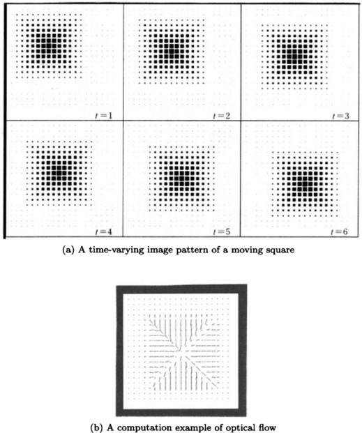
Figure 4.10 shows a time-varying image of a square moving across a screen (at six points of time) in two-dimensional Euclidean space and the optical flow obtained at t = 6. Note that there are many other methods for computing optical flow.
(b) Detecting the direction of movement using optical flow
Let us consider a method for determining the direction of movement of a surface as an example of feature extraction applying optical flow. Suppose, as in Figure 4.11, an observer with a single eye stands at the origin of three-dimensional Euclidean space and is looking at the pattern of a static surface S at distance r from the origin that is being projected onto the surface of the unit sphere (sphere with radius 1) around the origin. As you can see from Figure 4.11,
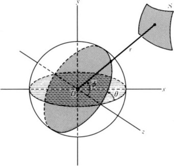
holds, where θ′ = dθ/dt, u = dx/dt, v = dy/dt.
If we substitute x = r sin ϕ cos θ into (4.9), we have
On the other hand, by using z = r cos ϕ,
where ![]() Now if we substitute r′ (xu + yv + zw)/r into (4.11),
Now if we substitute r′ (xu + yv + zw)/r into (4.11),
(4.10) and (4.12) are the angular velocity in the θ and ϕ directions, respectively. Therefore, they are the equations that need to be satisfied by the optical flow in spherical coordinates.
Now, suppose the observer at the origin moves at the speed –V in the z direction, facing the static surface S (see Figure 4.12). (Relatively, this is the same as the situation where the object is moving at a certain speed, facing the observer.) Since
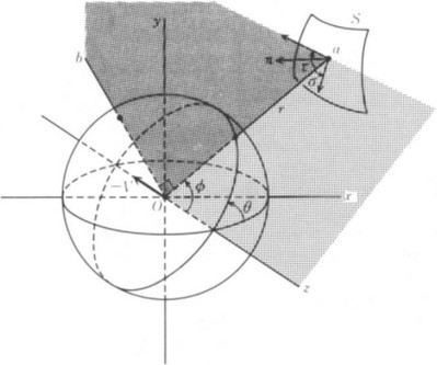
Figure 4.12 The direction of the surface based on the optical flow that is generated by going farther on the z axis.
we substitute them into (4.10) and (4.12) and obtain
Now let us compute the normal n of the surface S at a point a on S using the optical flow given in (4.13) and (4.14). First, let us consider the angles σ and τ on the planes aoz and boa that satisfy
σ and τ each represent the rate of change of the distance to the point a of the object with respect to ϕ and θ when the observer moves. The normal n of S can be computed using σ and τ. Now we differentiate (4.14) using ϕ and θ, respectively,
If we substitute these into (4.15) and (4.16), we get
(4.17) and (4.18) show that it is easy to obtain σ and τ from the optical flow in the ϕ direction. In particular, note that (4.17) and (4.18) can be computed independently of the speed of the observer V, the distance r between the observer and the object, and the rate of change of r, that is, ∂r/∂θ and ∂r/∂ϕ.
(c) Ill-posed problems and their regularization
As noted in (a) and (b), we cannot generally find a unique solution to a feature extraction problem based on optical flow. For example, in extracting the direction of a surface as in (b), we gave general equations for the flow using spherical coordinates in (4.10) and (4.12); however, by using only these equations, it is generally difficult to extract a feature such as the direction of the movement of a surface. To compute a specific flow, we need to introduce an external constraint, for example, an observer moving at a fixed speed along a coordinate axis (as we did in (b)). Also, in the method of computing flow explained in (a), (4.3) is an equation to be satisfied by the flow; however, there are infinitely many flows that satisfy (4.3). Therefore, in (a) we used the external constraint that makes the flow locally smooth.
In this subsection, we will have a more general discussion of the problem of not being able to determine a feature uniquely based only on optical flow. The reason why we cannot compute flow determining a feature uniquely using only data provided by the pattern function is that a visual system is a special information processing system that transforms three-dimensional information into two-dimensional information and then reconstructs the three-dimensional information. We can assume that the visual system determines the three-dimensional information uniquely by constraining the information from outside by the structure of the system itself. The methods explained in (a) and (b) are special cases of formalizing the idea that the visual system solves an insufficiently constrained problems. Below we will give a general description of feature extraction as an insufficiently constrained problem and methods for solving such a problem.
(1) Ill-posed problems
When a unique solution to a problem P exists and is continuous in the initial conditions, we call P a well-posed problem. Otherwise, we call P an ill-posed problem. For example, ordinary linear differential equations satisfying appropriate conditions on continuity are well-posed problems, while simultaneous algebraic equations with more variables than the number of equations are generally ill-posed problems. Feature extraction by the visual system can be regarded as a kind of ill-posed problem.
(2) Calculus of variations and regularization
Let us consider the calculus of variations as a basic method for solving ill-posed problems. First, consider the problem P of obtaining a vector y that satisfies the simultaneous linear equation
for a given data vector x, where A is a linear operator.* When y is not determined uniquely for x (for example, when the inverse of the coefficient matrix A does not exist for the simultaneous linear equations in (4.19)), we can introduce another constraint for y and determine y uniquely “as much as possible.” For example, for an arbitrary linear transformation B, we can choose y to minimize the norm ||By||2. In this case, the original problem P can be formulated as the following problem.**
This is a problem in the calculus of variations using a quadratic functional, and λ is the undetermined Lagrange multiplier. As we assumed above, if A and B are linear operators and ||⋅|| is the square norm, a unique solution exists and it is continuous in the initial conditions. In other words, this problem is a well-posed problem. To transform a problem that is originally ill-posed into one that is well-posed is called regularization of the ill-posed problem, and λ is called the regularization parameter.
(3) Applying regularization to pattern recognition
Regularization can be applied to many pattern recognition problems including feature extraction. Some applications are shown in Table 4.1.

Let us consider the detection of an edge. Let i(x) be the quantized value of a pattern element, f(x) be the original pattern function, and Q be the sampling operator for f(x). Regularization, in this case, can be stated as the problem of reconstructing f(x) from the given quantized data i(x) under the condition that f(x) be as smooth as possible. In other words, if we represent this regularization problem in the form of a variation problem, it becomes the problem of finding an f(x) that gives the following minimum value:
where fxx(x) is the second-order differential of f(x).
The problem of reconstructing the original visual pattern from moving image data can be formulated similarly, provided we use, as a constraint, the condition that makes the inner product of the gradient Δf of the pattern function and the velocity vector V as close as possible to ft, the change of the intensity over time. This condition corresponds to (4.3).
Also, the regularization problem for optical flow in a region in Table 4.1 corresponds to the result described in (a). Furthermore, the problem of reconstructing the location of the surface of an object can be formalized as the regularization problem of obtaining the smoothest f(x, y) that makes the quantized sample Q(f(x, y)) of the surface coordinate f(x, y) have a value as close as possible to the depth d(x, y). For color, the problem of obtaining the intensity distribution that represents the distribution of the intensity data Iν well and makes the change in intensity minimum can also be obtained. The regularization problem of computing optical flow from contours of a pattern function can be formulated as the problem of obtaining, under the condition that the velocity vector V changes as smoothly as possible on the contours, the V for which there is the smallest difference between its projection toward the normal V · N (N is the unit vector to the normal direction) and VN(s), the normal direction component of V, when VN(s) (s is the length of a contour) is given as data.
Many other problems of visual pattern recognition are known to be for-malizable as regularization problems.
(4) The characteristics of pattern recognition using regularization
The problems summarized in Table 4.1 have the following two characteristics:
(1) The regularization problem can sometimes give a good explanation of the visual information processing of an organism.
(2) Some neural network algorithms, similar to those explained in Chapter 10, can be used to solve regularization problems using quadratic functional. Also, those problems can be solved using linear analog circuits.
Optical illusion is an example of (1). For example, there are cases in which a horizontal optical flow appears as a vertical flow in the solution to a regularization problem. This is a phenomenon similar to the one that occurs when we see a rotating barber’s sign. (2) suggests that the method of using regularization may give a fast algorithm. This is an important characteristic that may lead to the application of highly parallel computers to these problems.
4.6 Representing a Boundary Line
So far we have described methods for feature extraction in pattern recognition. These methods can be regarded as algorithms that generate and transform representations of features. However, we have not systematically explained how to represent the extracted features. From this section through Section 4.8 we will describe methods for representing features, especially boundaries, regions, and solid bodies. First, we will provide a method for representing a boundary line in two-dimensional Euclidean space.
(a) Representation using polygonal line approximation
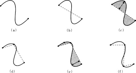
When we can assume that the boundary of an object is a continuous, smooth curve, we can represent this boundary approximately by using a linear polygonal line. For example, Figure 4.13 shows the use of a polygonal line approximation for a curve.
An algorithm for obtaining a polygonal line approximation for a given curve is as follows:
Algorithm 4.9(obtaining a polygonal line approximation of a curve)
[1] Make a segment by joining both ends of the curve, and let the segment be the initial state of a polygonal line approximation. (Generation of an initial segment)
[2] Do the following substeps for each segment of the polygonal line. (Improvement of the representation)
[2.1] Draw a perpendicular line from each point of the curve to the segment.
[2.2] If the length of the longest perpendicular line is smaller than a given threshold value, then stop. Otherwise, replace the original segment with the polygonal line approximation in two segments with an end point on the curve that makes the longest perpendicular line at end points.
[3] If [2.2] stops for all the segments in [2], stop the algorithm. Otherwise, go to [2]. (Recursive application)
(b) Chain code representation
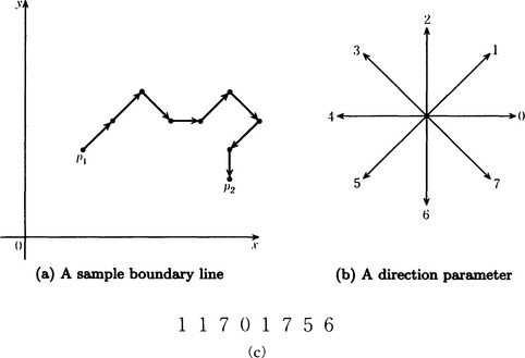
Let us consider a boundary made of segments such that the direction of neighboring pattern elements along the boundary that are attached to each other can be represented using a parameter for expressing some particular direction. For example, suppose we have the boundary shown in Figure 4.14(a). If we define the direction parameter to have eight values as in Figure 4.14(b), we obtain the series of direction parameter values shown in Figure 4.14(c) from point p1 to point p2. Such a series is generally called a chain code, and representing a boundary using a chain code is called chain coding.
A chain code representation has the following characteristics:
(1) It can compress information as compared to the original boundary data.
(2) The chain code can be used easily to restore the original boundary data.
(3) If we take the first-order differences of the chain code (differences of neighboring pairs of parameter values in the code modulo the number of direction parameters), the obtained representation becomes invariant under rotation of the boundary. Using this characteristic, we can judge the similarity of two boundaries that do not change under rotation.
(4) If the boundary is closed (that is, two end points coincide), it is easy to compute the area of the surrounded region.
(5) We can easily find a segment of certain length (and a segment of shorter length than that) whose end is an end point of the boundary. This characteristic can be used in eliminating noise.
(6) We can easily find the common part of two boundaries. This characteristic can be used in merging regions with a common boundary.
For example, with regard to (4), an algorithm for obtaining the area from the chain code representation of a closed boundary is the following when there are four direction parameters, up, down, right, and left:
(c) Fourier series expansion
We will explain the method for representing a boundary that is a continuous curve using a Fourier series expansion for the amplitude of the tangential line. Suppose the boundary l is a continuous closed curve. We write θ(s) for the amplitude of the tangential line at a point whose distance is s along l from the initial point on l as shown in Figure 4.15. Furthermore, if we let L be the whole length of l and let
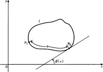
then ![]() becomes a periodic function of period L. If we do a Fourier series expansion of
becomes a periodic function of period L. If we do a Fourier series expansion of ![]() , we obtain
, we obtain
Therefore, we have represented the original boundary using the amplitude of the tangential line at the initial point and the Fourier coefficients ak and bk (k = 0,1,…).
As you can see from this example, we have obtained not only the boundary but also a representation for the figure surrounded by the boundary itself. So, if we use the values of the Fourier coefficients, we can relatively easily judge the similarity of two figures or distinguish the shape of a figure. Also, we can restore the original function from the values of the Fourier coefficients. Therefore, in the above method, we can restore the original boundary just by remembering the values of the Fourier coefficients (and the value of the amplitude of the tangential line at the initial point). In this sense, we sometimes call the Fourier coefficients in the Fourier series expansion the Fourier descriptor.
(d) Other methods
There are many other methods for representing a boundary. The cubic spline function approximation explained in Section 3.4 is often used as a method for approximating a boundary given a set of sample points of a curve. Other methods include using conic sections and representing the boundary using a binary tree with rectangles of various sizes and directions as nodes.
4.7 Representing a Region
We will explain some methods for representing a region in two-dimensional Euclidean space.
(a) x-coordinate and y-coordinate representations
First, we will describe the x-coordinate and y-coordinate representations. We start by quantizing a rectangle in the (x, y) plane that includes the given region. For the (quantized) interval of the x-axis [x0 ± nΔx, x0 ± (n + 1)Δx](n = 0,1,…, Nx), we enumerate quantized sections that include a pattern element whose value is not 0. For example, let us look at the region shown in Figure 4.16(a). This region, using the above method, can be represented as the list of names of sections shown in Figure 4.16(b). Each element of this list consists of a list whose first element is the the name of a section on the x-axis and whose second and later elements consist of lists of two elements, the name of a quantized section on the y-axis where the region begins and the name of a section on the y-axis where the region ends.
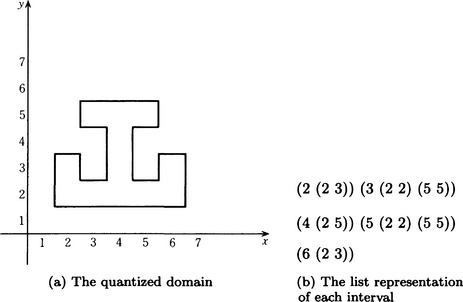
A list representation indexed by the names of the quantized sections that contain the region along the x-axis is called the x-coordinate representation of the original region. Similarly, a list representation indexed by the names of the quantized sections along the y-axis is called the y-coordinate representation of the original region. Since the x-coordinate representation and y-coordinate representation are simple enough to be easily generated from data of the region, they are often used to represent a region.
(b) Quad-tree representation
The x-coordinate and y-coordinate representations are methods for representing a region at the level of each pattern element composing the region and, thus, are one-level representations. On the other hand, there are methods for representing regions using a hierarchical structure of partial regions. As a popular method of this kind, we will describe the quad-tree representation.
Suppose a region in the (x, y) plane is quantized along the coordinates as in (a). Let us consider the following multilevel structure whose nodes are given a value. First, we define the lowest level that corresponds to the level of each pattern element. Next, for each set of four neighboring pattern elements at this level, we provide a new pattern element at one level higher. When the values of the four original pattern elements are all 1 (that is, all included in the region to be represented), we set the value of the new pattern element to 1. Also, when the values of the original four pattern elements are all 0 (that is, they are not included in the region to be represented), we set the value of the new pattern element to 0. Furthermore, if they do not belong to either case, in other words, when the four neighboring pattern elements have both values, 0 and 1, we set the value of the newly provided pattern element to 0.5. By repeating this operation to create superordinate levels, pattern elements in higher levels are generated; as a result, we obtain the pattern represented using a multilevel structure in that the whole pattern is represented by one pattern element in the highest level.
Let us consider the pattern shown in Figure 4.17(a). Suppose that the pattern elements represented as ![]() have the value 1 and other elements have the value 0, and the set of pattern elements whose value is 1 is the region. The multilevel structure for this pattern is illustrated in Figure 4.17(b), where
have the value 1 and other elements have the value 0, and the set of pattern elements whose value is 1 is the region. The multilevel structure for this pattern is illustrated in Figure 4.17(b), where ![]() ,
, ![]() ,
, ![]() represent the values 1, 0.5, 0, respectively.
represent the values 1, 0.5, 0, respectively.
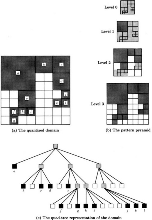
The representation of a pattern using a multilevel structure as above is called a pattern pyramid. In the case of a visual image pattern, it is called a (visual) image pyramid.
Considering the hierarchical structure that corresponds to a pattern pyramid, we can define a tree where the highest level of the pyramid corresponds to the root node. When the pattern element is ![]() or
or ![]() , the pattern element corresponds to a leaf of the tree. When the pattern element is
, the pattern element corresponds to a leaf of the tree. When the pattern element is ![]() , it corresponds to an intermediate node that has edges connected only to neighboring levels. For example, for the pyramid shown in Figure 4.17(b), we can obtain the tree structure shown in Figure 4.17(c). A tree generated in this way has the structure of a quad-tree, where every node except a leaf has four child nodes. This tree structure can easily be represented on a computer as a list. Also, by counting the number of
, it corresponds to an intermediate node that has edges connected only to neighboring levels. For example, for the pyramid shown in Figure 4.17(b), we can obtain the tree structure shown in Figure 4.17(c). A tree generated in this way has the structure of a quad-tree, where every node except a leaf has four child nodes. This tree structure can easily be represented on a computer as a list. Also, by counting the number of ![]() , we can compute the area of the original region. Furthermore, we can choose a representation with cruder levels rather than using the level for the original pattern elements. We can also easily pick nodes of appropriate depth in the tree structure. However, it is not easy to do geometric operations such as rotation, expansion, and contraction of the region.
, we can compute the area of the original region. Furthermore, we can choose a representation with cruder levels rather than using the level for the original pattern elements. We can also easily pick nodes of appropriate depth in the tree structure. However, it is not easy to do geometric operations such as rotation, expansion, and contraction of the region.
(c) Skeletal representation
Extracting a long thin region, or a set of connected line or curve segments, that is a subset of the original region and that in some ways maintains the same distance from the boundary is called skeletonization of the original region. A representation obtained by skeletonization is called a skeletal representation. To generate line segments going through the center of the region and preserving the connectivity of the region is called linear skeletonization, and a representation obtained by linear skeletonization is called a linear skeletal representation. This method of representation is appropriate for representing a region composed by stick-shaped subregions such as a human body.
4.8 Representation of a Solid
Let us consider the representation of a pattern obtained from a solid object in three-dimensional Euclidean space (we will call this just the representation of a solid). Methods of representing solids are roughly divided into the following three groups:
We will explain each group below.
(a) Representation using boundary lines
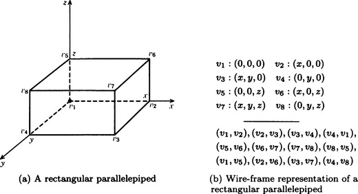
A well-known method of representation using boundary lines is the wire-frame representation described in Section 2.2. For example, the rectangular parallelepiped shown in Figure 4.18(a) can be represented using the coordinates of each vertex and the neighbor relation of vertices determined by the sides. Such a representation is shown in Figure 4.18(b). If we consider x, y, z as variables, we can look at Figure 4.18(b) as representing a general rectangular parallelepiped that is parallel to the coordinate axes and with one vertex at the origin.
(b) Representation using boundary surfaces
The winged-edge model method, the surface patch method, and the spherical function method are methods of representation using boundary surfaces.
(1) The winged-edge model method
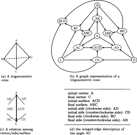
The method of representing a solid by a graph that assigns its surfaces, angles, and vertices as the nodes and takes the neighbor relations as edges is called the winged-edge model method. (Sometimes this method does not use the surfaces of a solid, but just some parts of the solid and their neighbor relations.) For example, the triangular conic shown in Figure 4.19(a) can be represented as the graph in Figure 4.19(b).
In the winged-edge model, the attribute-value pair for each node in the graph can be stored separately in the following form:
(i) Vertex: the coordinate location of the vertex in the object-centered system of coordinates and the observer-centered system of coordinates.
(ii) Side: the topological relation of the side with the neighboring vertices, sides, and surfaces.
(iii) Surface: surface features such as the orientation of the surface (can be represented as a normal vector), reflection rate, texture, color, and so on.
For example, for the side AC in the triangular conic shown in Figure 4.19(a), the relation with the vertices, angles, and surfaces shown in Figure 4.19(c) can be stored as the data given in Figure 4.19(d). As in Figure 4.19(d), it is usual to describe an angle as turning in the counterclockwise direction relative to the observer. The winged-edge model method not only gives simple representations but also can easily describe features of the surface and the location of the solid.
(2) Surface patch method
When a surface of a solid is a curved surface, we need to construct a representation that takes into consideration the curvature of sides and surfaces. This generally requires a complicated representation. As one of the simplified methods, we can approximate the surface by patching together some parts of planes or of curved surfaces. This method is called the surface patch method. This general method includes a method for generating partial curved surfaces from the three-dimensional information about the original solid and a method for imagining a curved surface with four sides as a partial curved surface and approximating those sides using B-spline functions.
(3) Spherical function method
The method of representing a surface of a solid as a function on a sphere is called the spherical function method. For example, there is a method for using a sphere where the distance between its center and a point on the surface of a solid is a function of its direction vector. Such a sphere is called a Gaussian sphere. We can project the normal vector at each point on the surface of a solid to the surface of the Gaussian sphere and let the normal vectors in the same direction take their vector sum. This vector field is generally called the extended Gaussian image. The representation method using the extended Gaussian image is one kind of spherical function method.
The extended Gaussian image preserves the congruent relation between convex* solids. Using this property, we can judge the congruency of two convex solids. There are also other spherical function methods, including methods using spherical harmonic functions.
(c) Representation using volume
We can also represent a solid by using features of three-dimensional volumes rather than local features in one- or two-dimensional space such as edges or surfaces. Using volume is more appropriate for representing a complex object since it can create macroscopic, concise representations. We will explain the generalized cylinder method and constructive solid geometry, two popular representation methods using volume.
(1) The generalized cylinder method
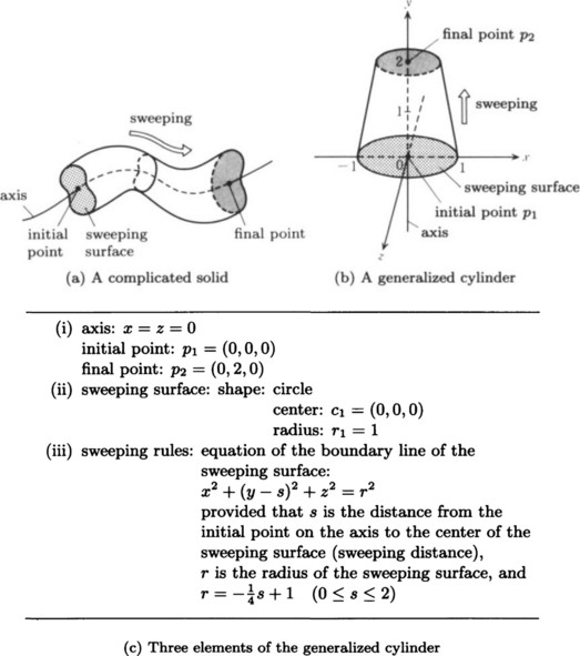
The solid obtained by generalizing the bottom surface and each cross section of a cylinder from a circle to a general simple closed curve or by changing the central line from a straight line segment to a curve segment is called a generalized cylinder. The method of representing a solid by using the position of its parts, assuming that the original solid is made of some pieces, and by representing each piece as a generalized cylinder is called the generalized cylinder method. We can construct a generalized cylinder by assigning a curve in three-dimensional Euclidean space, E3, as a spine and specifying a moving surface orthogonal to this spine by allowing the surface to change its shape as it moves from one end point of the spine to the other end point (such a move is called sweeping). Thus, a generalized cylinder can be described using the following elements:
(i) A curve in E3, in other words, the spine, its initial point, and its final point.
(ii) The shape of a sweeping surface at the initial point of the spine.
(iii) A rule for deciding how the shape changes during the sweep.
For example, the generalized cylinder shown in Figure 4.20(b) can be described as in Figure 4.20(c).
One characteristic of the generalized cylinder method is that we can easily compute the volume of a solid. Let p1, p2, and s be the initial point of spine, its final point, and the distance along the spine from p1, respectively. Also, let S(s) be the area of the surface orthogonal to the spine, or the section, at distance s from p1 along the spine, and let L(s) be the length of the boundary of the surface. Furthermore, let τ be the length of the arc on the boundary and represent a point p on the boundary as p = (x(s, τ), y(s, τ), z(s, τ)) using s and τ as parameters. The volume V of the generalized cylinder can be obtained by
For example, for the generalized cylinder in Figure 4.20(b),
Therefore
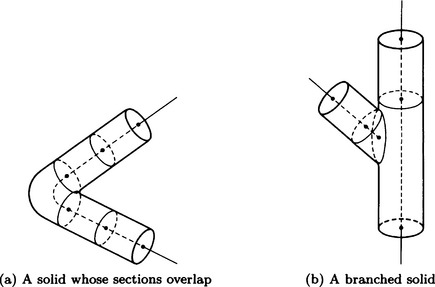
Using the generalized cylinder method, it is known that, if we look at the three-dimensional orthogonal coordinate system called the Frenet frame as a local coordinate system with each point on the spine as the origin, we can easily obtain much information about a pattern. The generalized cylinder method is suitable for representing a solid whose spine is not very bent. It can also easily transform the slope of a solid by changing values of parameters. However, it is hard, using the generalized cylinder method, to represent a solid that is so bent that sections overlap as in Figure 4.21(a) or a solid branched as in Figure 4.21(b).
It is not easy to generate a generalized cylinder from a pattern function. One method for doing that is to obtain a skeletal representation of the region using some linear skeletonization algorithm and find the shapes of the sections at several points along this skeleton. However, with this method, it is difficult to generate completely a representation like Figure 4.20(c). So the generalized cylinder method is often used as a method for representing a three-dimensional model to be stored in a knowledge base, rather than for representing a visual pattern.
(2) Constructive solid geometry
If we assume that a solid is made up of some solid primitives, we can reconstruct the original solid from them by defining their transformation operations. As solid primitives, we usually use rectangular parallelepipeds, circular cylinders, spheres, and generalized cylinders as described in (1). As transformation operations for a solid primitive, we use combinatorial operations such as sum and difference and operations on movement. This method of representing solids is called constructive solid geometry.
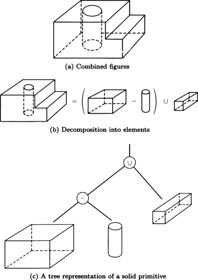
For example, the solid shown in Figure 4.22(a) can be constructed by the combinatorial operations of solid primitives shown in Figure 4.22(b). Or, using a tree structure, we can use the tree shown in Figure 4.22(c), which has solid primitives at its leaves and operators as intermediate nodes.
Using constructive solid geometry, we can represent not only individual solids but also a class of solids by parameterizing the attributes of the solid primitives (such as the length of a side of a rectangular parallelepiped). If we combine this method with the generalized cylinder method described in (1), we can represent many kinds of solids like those in Figure 4.23. However, in order to use constructive solid geometry we need to know the positional relation among the solid primitives that we used, as well as information about their locations, relative angles, and extent.
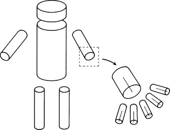
Figure 4.23 Combining constructive solid geometry with the generalized cylinder method (modified from Marr and Nishihara, 1978).
4.9 Interpretation of Line Drawings
In this chapter we have so far explained methods for extracting features and representing them in a computer. In particular, we gave methods for representing solids in Section 4.8. In this section we will explain a method for finding, in a pattern consisting of overlapping solids, what kinds of solids are contained in the pattern and where they are relatively positioned.
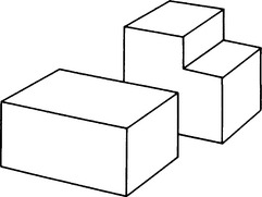
A pattern including more than one object is called a scene. In particular, a scene including only polyhedra is sometimes called a polyhedral scene. Finding the structure and attributes of objects or positional relations among objects in a scene is called scene analysis. Scene analysis is one of the important problems in pattern recognition. Here we will look at the simplest case, where the scene is a line drawing as in Figure 4.24. To obtain a line drawing from a given pattern function, we can combine and use the appropriate feature extraction methods described so far. Let us suppose we have already obtained a line drawing and think about a method for finding the objects contained in the line drawing and their relative positions. Scene analysis for a line drawing in this sense is called an interpretation of the line drawing.
(a) The Guzman method
A method that is often used for interpreting a line drawing is to classify the shape of each vertex and its neighborhoods, generate a graph based on the connective relations among the classified shape characteristics for vertices (called vertex elements), and interpret the line drawing by matching this graph and a graph that corresponds to a solid primitive. Of such methods, we will first describe one of the classics, the Guzman method.
Let us consider the six kinds of vertex elements shown in Figure 4.25(a). By using these vertex elements, we can represent a line drawing using a graph based on the connection among elements. On the other hand, we represent each solid primitive using a graph whose nodes are vertex elements, so that, if any subgraph of the graph for the original line drawing matches the graph of a primitive solid, we can recognize the solid primitive in the original line drawing. For example, we can represent the line drawing in Figure 4.24 as the graph G1 in Figure 4.25(b). On the other hand, suppose the graph G2 for a rectangular parallelepiped shown in Figure 4.25(c) is given as the graph of a solid primitive. If we ignore the nodes of G1 that correspond to the T-shaped vertices, G2 matches a subgraph of G1.
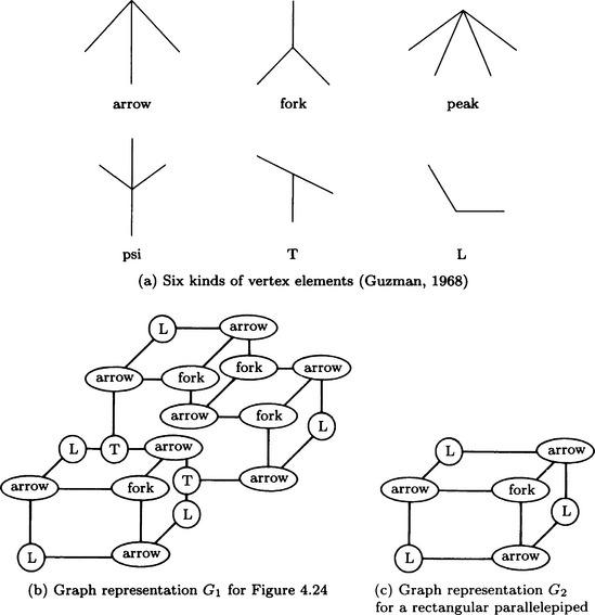
By repeating this sort of matching with the graphs of solid primitives, we can interpret a line drawing as more than one solid primitive. The Guzman method, as illustrated in the above example, is not always perfect in matching two graphs and generally requires rules for ignoring some nodes. Since such rules depend largely on the structure of each graph, there can be many exceptions for matching. Also, since this is a method for directly matching two graphs, a lot of calculation is required to interpret a complicated line drawing.
(b) Huffman-Clowes method
Whereas the Guzman method matchs graphs based on the shapes of vertex elements, there are methods for interpreting line drawings by making use of properties of boundary lines. One of these methods is the Huffman-Clowes method. We start by assigning one of the labels +, −, or > to a boundary line in a line drawing.
(1) If a boundary line is convex from the viewpoint of the observer, assign +.
(2) If a boundary line is concave from the viewpoint of the observer, assign −
(3) If a boundary line has one of its adjacent surfaces* hidden, assign >, provided that the hidden surface should be on the left side of the line and the surface that is visible should be on the right side of the line.
(The Clowes method also uses ↑ as the label for the direction of a shadow line.)
If we use these rules for assigning labels, there will be only 16 possible labelings for a vertex of a polyhedron whose vertex connects only three surfaces (trihedral-vertex polyhedron). Figure 4.26 shows the 16 labelings. In the case of a trihedral-vertex polyhedron, the Huffman-Clowes algorithm assigns one of the vertex elements shown in Figure 4.26 to each vertex of a given line drawing. However, this method uses only local information about the shape of each vertex and its neighborhood, so it may label meaning-less line drawings without contradiction or assign an impossible label in a meaningful line drawing.
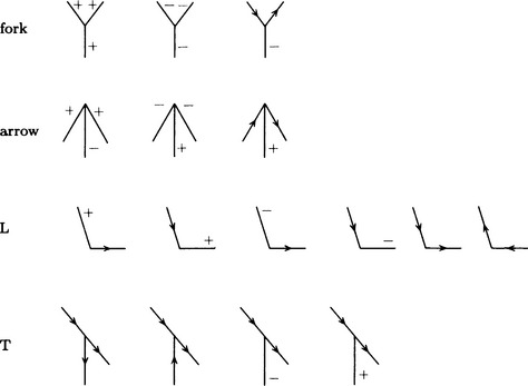
Figure 4.26 Huffman’s labeling for a trihedral-vertex polyhedron (Huffman, 1971).
(c) The Waltz method
One shortcoming of the Huffman-Clowes method is that the algorithm for labeling may not be applied to all possible line drawings. The Waltz method, though like the Huffman-Clowes method it is based on labeling boundary lines, uses a more farsighted global algorithm for labeling a line drawing, which is called constraint filtering. Let us look at an outline of the algorithm.
Algorithm 4.11(1) (labeling a line drawing using the Waltz method- outline)
[1] Enumerate all possible labelings for each vertex in a line drawing. (Enumeration of labelings)
[2] For each line segment in the line drawing, remove any labeling from the labelings enumerated in [1] that does not satisfy the following constraint. (Constraint filtering)Constraint on labeling: any line segment has to have the same label on both end points.
[3] Repeat [2] until all the line segments satisfy the constraint. (Relaxation)
The algorithm outlined above is an instance of an optimization method called the relaxation method. Let us look at this algorithm in more detail from the standpoint of a relaxation method.
Algorithm 4.11(2) (labeling a line drawing using the Waltz method)
[1] Name the vertices of a given line drawing 1,…, n and do the following substeps for each pair of vertices i, j:
[1.1] Set rik = 1 when assigning label k to vertex i is possible; otherwise set rik = 0.
[1.2] When the vertices i, j are neighbors and labeling k, l is possible for i, j, respectively, do the following:
[1.2.1] If labeling k, l gives the same label to the segment that joins i, j, set s(i, j, k, l) = 1. Otherwise, set s(i, j, k, l) = 0.
[2] Enumerate possible labelings kil,…, kini for each vertex i. (Enumeration of labelings)
[3] For any vertex i and its neighboring vertex j, if s(i, j, k, l)rjl = 0 is true for all l = kj1, change the value of rik from 1 to 0. (Constraint filtering)
[4] Do [3] for each vertex i and repeat this operation. (Relaxation)
Not only does the Waltz method introduce constraint filtering into the Huffman-Clowes method, it also can interpret a line drawing that includes shadow lines and cracks. The number of locally possible labelings will increase in a line drawing that includes shadow lines and cracks, but by using an algorithm with constraint filtering our experience tells us that only one or at most a few possible interpretations will be obtained that keep consistent labelings for all segments.
Section 5.2 will explain the Waltz method in more detail with examples.
(d) The Kanade method
The methods we described so far can be used on line drawings of scenes built out of convex polyhedrons. The Kanade method is a constraint filtering algorithm that can interpret not only such line drawings but also line drawings including folded-up polyhedrons (the origami world). This method, using labelings with the vertex elements shown in Figure 4.27, performs constraint filtering similar to that in the Waltz method. For example, the result of interpreting the line drawing of a box (shown in Figure 4.28(a)) is shown in Figure 4.28(b).
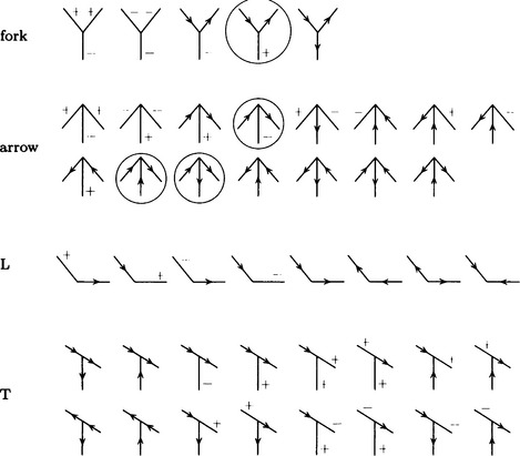
Figure 4.27 Labeling for the origami world by Kanade (see the text for the ones with a circle) (Kanade, 1980).
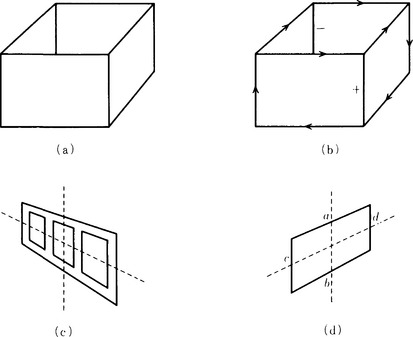
Figure 4.28 Interpretations of line drawings by the Kanade method (Kanade, 1980).
In Figure 4.28(b) there are four vertex elements that are not included in the list of vertex elements for the Huffman-Clowes method. They are circled in Figure 4.27. Those elements are a consequence of allowing folded-up polyhedra.
On the other hand, if we think of a line drawing as the projection of a solid in three-dimensional Euclidean space onto two-dimensional Euclidean space E2, the resulting constraints can be used to reduce the multiplicity of interpretations. In particular, if we use the following two heuristic constraints, we can reduce the number of interpretations in the origami world.
(1) Skew symmetry: we assume that, in E2, a figure that is symmetrical in an oblique coordinate system is symmetrical in the original orthogonal coordinate system in E3.
(2) Preserving parallelism: we assume that two line segments that are parallel in E2 are also parallel in E3.
For example, the object in Figure 4.28(c) is symmetrical in an oblique coordinate system, and it is assumed by (1) to be symmetrical in the orthogonal coordinate system in E3. Also, by (2), the parallel segments in Figure 4.28(d), a and b, or c and d, are assumed to be parallel in E3.
Summary
This chapter described algorithms for extracting features from a visual pattern.
4.1. The zero-crossing method and the difference operator method can be used to detect an edge.
4.2. The edge tracing method, the edge prediction method, and the Hough transformation method can be used for extracting boundary lines.
4.3. The splitting method, the merging method, and a method that combines both can be used for extracting a region.
4.4. Structure analysis, statistical analysis, and the texture gradient method are used for texture analysis.
4.5. Optical flow is used for detecting movement.
4.6. Many pattern feature extraction problems can be formulated as regularizations of an ill-posed problem. Detection of movement using optical flow is one example.
4.7. A boundary line can be represented by a polygonal line approximation, a chain code, or a Fourier series expansion.
4.8. A region can be represented by an x-coordinate representation, a y-coordinate representation, a quad-tree representation, or a skeletal representation.
4.9. A solid can be represented using boundary lines as in a wire-frame representation; using surfaces as in the winged-edge model method, the surface patch method, or the spherical function method; and using volumes as in the constructive solid geometry and the generalized cylinder method.
4.10. The Guzman method, the Huffman-Clowes method, the Waltz method, and the Kanade method are used for scene analysis of line drawings.
Exercises
4.1. Explain how the formula in Section 4.1(a), k(x, y) = ∇2H(r)*f(x, y), should be transformed to run the zero-crossing method on a computer. How many multiplications and exponentiations are necessary to compute the zero crossing, using the transformed formula?
4.2. Solve the example problem for the Hough transformation described in Section 4.2(c) (see Figure 4.7) using polar coordinates (r, θ) as the parameter space.
4.3. Write an algorithm for finding the skeletal representation of a region represented by a two-dimensional bit pattern.
4.4. Describe the difference between wire-frame representation and representation by the winged-edge model method. Also explain the merits of combining these two kinds of representation.
*The simplest example of a linear operator is the coefficient matrix of simultaneous linear equations. The arguments here encompass more general instances and apply to a wide range of linear operations.
**It can also be defined as the problem of finding a y that minimizes ||By||2 and satisfies ||Ay − x|| < ∈ for some ∈ > 0.
*We say a set D in n-dimensional Euclidean space is a convex set if, for any x1, x2 ∈ D and real number μ ∈ [0,1], μx1 + (1 − μ)x2 ∈ D. A convex solid is a convex set in three-dimensional Euclidean space.
*Sometimes the word “face” is used instead of “surface,” particularly for polyhedral solids. But we use the word “surface” consistently in this book.