
Pattern Understanding Methods
One of the goals of pattern recognition is to find an object included in a pattern as well as its attributes and its relationship to other objects in the pattern. This is generally called pattern understanding. Attributes and relationships of objects can be represented by the methods described in Chapter 3. The job of pattern understanding is to generate representations of these attributes and relationships from a given representation of a pattern or from the representation of extracted features. Pattern understanding requires knowledge about an object. Feature extraction methods can recognize the boundaries and regions included in a pattern, but they cannot understand the pattern: understanding a pattern requires knowledge of the corresponding objects. This chapter will explain methods of pattern understanding based on knowledge of objects. Pattern understanding, in this sense, requires algorithms for matching stored knowledge and extracted features and methods for controlling the process from feature extraction to pattern understanding. This chapter discusses both of these problems in order.
5.1 Pattern Understanding and Knowledge Representation
Before we explain the methods of pattern understanding, we need to think about how the knowledge necessary for understanding can be represented in a computer. In this section we discuss knowledge representation methods appropriate for pattern understanding.
(a) What is knowledge representation?
We need knowledge in order to understand what is in a picture. For example, if we have knowledge about roads and buildings, we understand that Figure 5.1(a) is a picture of a building. However, if we do not have enough knowledge, we will not understand what kind of picture it is. For example, some people may not understand what is in Figure 5.1(b).
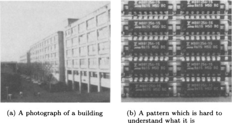
If we do not have knowledge about the shape of a building or a road, we cannot understand the pattern in Figure 5.1(a). In representing this knowledge, we can use a declarative representation, such as “the shape of a building from above is usually a rectangle” or “a road, from above, has a long and narrow belt shape,” or a procedural representation for connecting such knowledge to features such as boundaries and regions. Furthermore, this kind of knowledge becomes useful for pattern understanding only when it can be effectively used in conjunction with an inference mechanism that can generate the attributes of an object such as a building or a road or a relation between objects from a pattern and its features. A framework for representing knowledge in a computer, so that the information necessary to carry out intellectual activities such as pattern understanding and an inference mechanism for actually accomplishing this intellectual activity satisfy the following three conditions, is called a knowledge representation:
(1) It can represent human knowledge possibly as it is.
(2) The inference system is highly efficient.
(3) It is easy to describe and modify knowledge and to understand the descriptions.
It is convenient to use symbols when representing human knowledge in a computer. Thus the representation methods using symbols, like lists, semantic networks, rules, and frames, are often used for knowledge representation. Knowledge represented using a declarative representation is called declarative knowledge, and knowledge represented using a procedural representation is called procedural knowledge.
(b) Basic techniques of knowledge representation
Here we provide the basic techniques of knowledge representation for pattern recognition.
(1) The representation of declarative knowledge using semantic networks
First let us consider, using an example, a method for representing declarative knowledge. Suppose we have an object “triangle.” Our declarative knowledge about the object “triangle” includes the attributes of triangles in general, their values, and their relation with other objects.* Consider the fact that there are three vertices in a triangle. This fact can be represented, if we represent a triangle by the symbol triangle and the attribute, the number of vertices, by the symbol number _of _vertices, as the following list of three elements:
If we represent the attribute that is the number of sides of a triangle using the symbol number _of _sides, the fact that a triangle has three sides can be represented as
In this way, if we represent each characteristic of an object in the form of a list
we can represent the characteristics of an object, or equivalently the object itself, as a set of such lists. This representation is one example of a semantic network.
Next, let us consider relations among objects. For example, an equilateral triangle inherits the general characteristics of a triangle. If we represent this inheritance relation using the attribute isa:, we can represent the relation between a triangle triangle and an equilateral triangle equilateral_triangle as the list
Also, the relation between “a triangle” and one of its sides is the relation that the side “is a part of” a triangle. If we represent this relation using the attribute partof:, we can represent the relation that the side ab is a part of the triangle abc using the list
Usually, isa: is called the superordinate-subordinate relation and partof: is called the part/whole relation. Both of these are often used in representing attributes of objects for pattern understanding.
On the other hand, we can think about the inverse relation of isa: or partof:. As opposed to the inheritance of a characteristic using the attribute isa:, we can represent the fact that a triangle is superordinate to an equilateral triangle as follows using the attribute supers::
This is the inverse relation to (equilateral_triangle isa: triangle). Similarly, the relation that a triangle abc has the side ab as a part can be represented as follows using the attribute haspart: :
So far, we have used the atom triangle and the list (triangle a b c) for representing a triangle and the triangle abc, respectively. The former is a general term representing the class of triangles; the latter is the particular triangle abc and represents one instance. Suppose we attach, to triangle, variables $x, $y, $z representing the three vertices as arguments. Then, we can represent the class of triangles as (triangle $x $y $z). The fact that (triangle a b c) is an instance of the class called (triangle $x $y $z) can be represented as follows using the attribute class::
If we represent the inverse relation of class: using the attribute instance:, we can represent the fact that the class (triangle $x $y $z) has the instance (triangle a b c) as follows:
Extending the above arguments, we can describe a general triangle (triangle $x $y $z), its instance (triangle a b c), and the equilateral triangle (equilateral_triangle $x $y $z) using the semantic network shown in Figure 5.2.
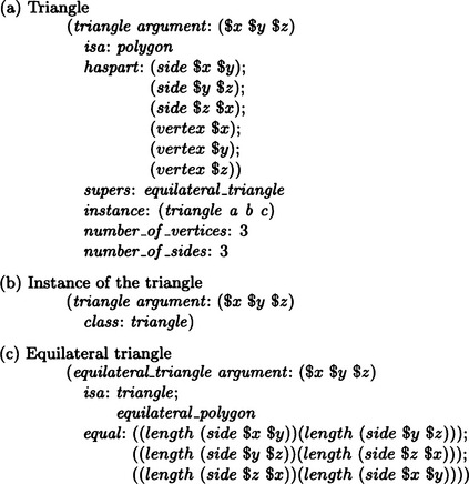
In Figure 5.2, we assume that $x, $y, $z are local variables defined only inside triangle but their scope extends to objects that inherit the properties of triangle. For example, since an equilateral_triangle is a triangle by virtue of the inheritance of the attribute isa:, the value of each attribute of triangle is inherited, with its variables, to equilateral_triangle. Therefore, equilateral_triangle, just like triangle, has (vertex $x), (vertex $y), (vertex $z) as its parts.
(2) Inference using a semantic network
Now, let us consider how we do inference using semantic networks. For example, how would we answer the question “how many sides does an equilateral triangle have?”? Suppose the equilateral triangle equilateral_triangle is represented as in Figure 5.2. If we check the value of its isa: attribute, we are led to triangle, and by looking in triangle we find that the number of the sides is three. Here, the attribute isa: means that the properties of the superordinate class triangle are inherited by the subordinate class equilateral_triangle.
As we noted in Chapter 2, the case of multiple inheritance causes problems when trying to do inference by inheritance. For example, the equilateral triangle equilateral_triangle could be thought of as having two different superclasses, equilateral_polygon and triangle. If we are to infer the number of the sides of an equilateral triangle, it must inherit its number of the sides from a triangle, not from an equilateral polygon. In this case, we can represent the number of sides explicitly as the value of an attribute of equilateral_triangle using the blocking method.
(3) Representing procedural knowledge using rules
Here we explain how to represent procedural knowledge for pattern understanding using rules. First we consider how to infer properties of an object from local features that can be extracted from a pattern. For this purpose, let us define the following production rules:
if there are two ![]() shaped figures among the extracted features
shaped figures among the extracted features
then conclude that there is a rectangular object made by extending the horizontal sides of ![]() and
and ![]()
if there are two line segments among the extracted features
and they cross each other obliquely
then conclude that the two line segments intersect orthogonally in three-dimensional space
These rules are not always logically correct. They are heuristic rules in the sense that they are likely to give correct results. Usually, procedural knowledge tells what to do in particular situations like this example. When representing knowledge for use in pattern understanding, we need to build a knowledge representation system that can understand various different kinds of patterns, and methods that can represent heuristic rules, like production rules, are often effective.
(c) Knowledge representation for pattern understanding
In this section we discuss some problems of knowledge representation as applied to pattern understanding and how we might solve them.
(1) Superordinate/subordinate relation between classes of objects
There are many different levels of representation for one pattern function, and there are different methods of representation for each level. The diversity of different representations is one of the most interesting and most difficult problems in knowledge representation for pattern understanding. For example, there are the level of pattern elements, the level of boundaries and regions, the level of an object’s attributes and relations among objects, and the level of scenes that may include many objects. Each of these levels requires its own representation methods. There are even different representation methods for the same level, like the chain code representation and spline function representation of a boundary line.
(2) The whole/part relation between objects
For pattern understanding, the whole/part relation between objects is a more complicated problem than it is for general knowledge representation. For example, in a usual semantic network the whole/part relation can be completely described by using the attributes partof: and haspart:. However, in pattern understanding, the relative spatial location and the topological connection of two objects or the number of parts of an object can be factors that determine the whole/part relation.
When representing the shape of an object that is closely tied to the whole/part relation, there may be many levels of representation as explained in (1). So the whole/part relation of knowledge representation when used in pattern understanding, especially the relation of spatial positions, requires a detailed representation method.
Let us look at the pattern of the “hammer” shown in Figure 5.3(a). A hammer as an object can be represented by the class hammer as shown in Figure 5.3(b). It has two parts, the class of “head of a hammer,” hammer_head, and the class of “handle of a hammer,” hammer_hand.
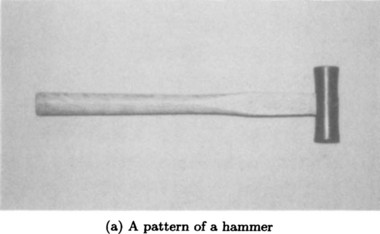
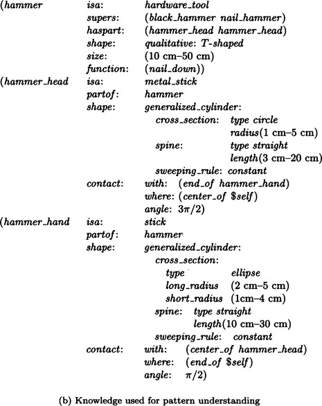
Figure 5.3(b) represents the shape of a hammer as the value of the attribute shape:. In other words, the value qualitative: T-shaped of shape: states that the general shape of a hammer is qualitatively T-shaped, where qualitative: is a subattribute of the shape:.
On the other hand, the class hammer_head uses the more quantitative representation of generalized cylinders for its value of shape:. We also use generalized_cylinder: as the subattribute for representing a generalized cylinder and cross_section:, spine:, sweeping_rule: as the sub-subattributes for representing the shape of a section, the shape of a spine, and a sweeping rule, respectively. The shape of hammer_hand is also represented using a generalized cylinder.
In Figure 5.3(b), the topological connection among objects is represented by the attribute contact:. The value of contact: is what part of two objects are connected and to what degree. We also make with:, where: and angle: subattributes representing “with” what object, “where,” and “at what angle” an object is connected, respectively. For example, the value of the attribute contact: in hammer_head gives that “the handle of a hammer” is connected to the end of “the head of a hammer” at its center with 270 degrees in a two-dimensional plane. $self is a variable that binds the name of the class in which it is defined.
The following are examples of spatial relations between two objects X and Y:
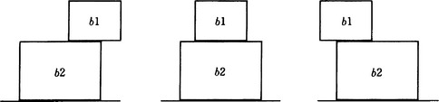
In general, there are many patterns that correspond to a given symbolic representation of a spatial relation. This is certainly true for two connected objects. For example, think about representing “box b1 is on box b2.” By thinking of b1 and b2 as instances of the class of boxes, box, this can be represented as an attribute-value pair on the instance b1, (b1 on: b2).
However, even if we are given this list, patterns corresponding to it will not be unique. For example, in Figure 5.4, (b1 on: b2) is used to represent both the case in which b1 is right on b2 and the case in which b1 is slightly off to the right or left on b2.
For this reason spatial relations like on: are more appropriately represented by a set of constraints that determine the position of corners of boxes. For example, if we regard b1 and b2 as two-dimensional rectangles and let (x1,y1) and (x2,y2) be the coordinates of two vertices on the bottom side of b1 from the left and (a1, b1) and (a2, b2) be the coordinates of two vertices on the top side of b2 from the left, we have the following feature level representation corresponding to the symbolic representation (b1 on: b2):
This is a set of constraints on the coordinates of the corners.
The method of using fuzzy sets is another way of representing spatial relations, though it will not be considered in this book. Knowledge of the correspondence between a symbolic representation and a feature level representation can itself be a powerful tool for finding a symbolic representation of an object and its relation to other objects from features extracted from a pattern.
(3) Hierarchical representation
For some purposes in pattern understanding we need only understand the rough structure of a pattern rather than analyze the whole in detail. If we do not know anything about what we are looking at before we try to understand a pattern, we could extract a crude representation first and then try to understand each part in more detail from that information. In order to use this method effectively, it is better to represent knowledge in a hierarchical fashion.
Figure 5.5 illustrates how to represent parts of a human body using generalized cylinders. Using this hierarchical representation based on the whole/part relation, we can first try to match classes at a high level in the hierarchy with the pattern at low resolution. If we succeed, then we can try to understand the more detailed parts by matching classes lower in the hierarchy with the pattern at a higher resolution.
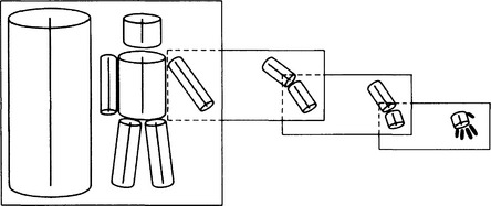
Figure 5.5 Representation of “a person” using generalized cylinders (modified from Marr and Nishihara, 1978).
(4) Knowledge representation for pattern understanding 1
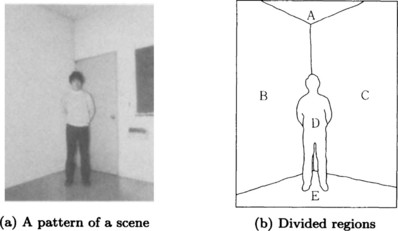
Here we give an example of knowledge representation used in pattern understanding. Suppose that by feature extraction, we have divided the scene shown in Figure 5.6(a) into regions as shown in Figure 5.6(b).
Also, let us suppose that a pattern understanding system has the following procedural knowledge in its rule base:
(i) If the region X is the uppermost region then conclude that X is a ceiling or the sky.
(ii) If the region X is the lowest region then conclude that X is a floor or the ground.
(iii) If the region X is a quadrangle and X is connected to both the uppermost and lowest regions then conclude that X is a wall.
(iv) If the boundary of a region X includes a curve and X is connected to both the uppermost and lowest regions then conclude that X is a forest.
(v) If the region X is connected to the lowest region and X is not connected to the uppermost region then conclude that X is a human being.
(vi) If a human being is included in the scene then conclude that the uppermost region is a ceiling.
Based on this knowledge, the problem is to infer what object corresponds to each of the regions, A-E, in Figure 5.6(b). Let us call the name of the object corresponding to the region A the label of A. Then the problem is to label the regions. In our example we examine the production rules from the top in order. If we use the inference method using ordered rules, we will obtain the following labeling:
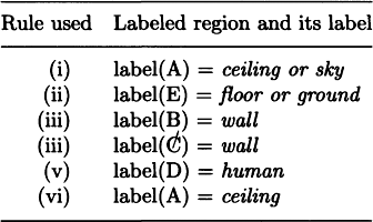
In other words, we can conclude that the regions A, B, C, and D can be regarded as a ceiling, a wall, a wall, and a human being, respectively. Since the region E can be thought of as either a floor or the ground, we have inferred that the scene in Figure 5.6(a) is a room containing a human being.
Of course, this result depends on the reliability of the knowledge used in making the inferences and may not be perfectly reliable. Also, this example is very simple and uses only one kind of knowledge representation. Even from our simple example, however, we see that we cannot understand a pattern merely with the feature extraction techniques described in Chapter 4. In order to know what exists in a given pattern, we need to build a pattern understanding system based on knowledge.
(5) Knowledge representation for pattern understanding 2
Now, let us consider a more realistic example of pattern understanding.
Consider the colored scene shown in Figure 5.7(a). First, we do feature extraction for the original pattern based on color and divide it into smaller regions as shown in Figure 5.7(b). By merging smaller regions around each bigger region, we obtain the final partition of regions shown in Figure 5.7(c).
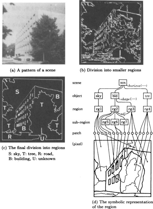
Figure 5.7 Pattern understanding based on knowledge. (Ohta, 1985)
If we represent each region obtained so far as a class, we obtain the symbolic representation of the pattern shown in Figure 5.7(d).
Next, based on knowledge, we try to label the regions partitioned as in Figure 5.7(c). We suppose that knowledge is represented by the semantic network and production rules shown in Figure 5.8. The semantic network represents declarative knowledge of the properties of objects and the relations among objects, whereas the production rules represent the procedural knowledge used for labeling.
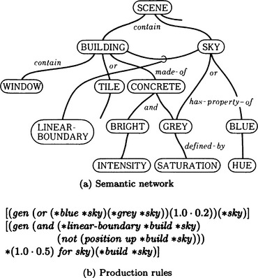
Figure 5.8 Knowledge for understanding the pattern in Figure 5.7. (Ohta, 1985)
In this case the pattern understanding system applies the production rules to the set of regions and, based on the knowledge in the semantic network, finds a plausible labeling of each region. That is, if we let n1,…, nk be the possible labelings for the region A, the plausibility of a labeling is is given by
Concretely, the plausibility is represented, for example, by label(A) = ((sky 0.7)(tree 0.2)(building 0.1)).
Next, by using a production rule (for example, the last rule in Figure 5.8), we select the labeling with the highest plausibility, generate the pair of a region and its label, and attach it to the partially constructed semantic network shown in Figure 5.7. In Figure 5.7, (…) means the parts to be attached.
5.2 Pattern Matching and the Relaxation Method
A pattern understanding system tries to find the attributes of the objects in a pattern or relations among such objects using knowledge represented by the methods explained in Section 3.1 and the features extracted from the pattern. In this section, we will describe an algorithm for matching knowledge against features.
(a) Properties of pattern matching in pattern understanding
Matching in pattern understanding, unlike matching in symbolic processing, needs to take the following points into consideration:
(1) Since local features of a pattern usually match many different pieces of knowledge, we need to do matching based on the global structure obtained from local features.
(2) We need to attempt matching at various representation levels of a pattern.
(3) Since features of a pattern usually include noise, we need a matching algorithm applicable to data including noise.
(b) The relaxation method
Let us look at a relaxation method that is a representative algorithm for obtaining global structure from a set of local features. The purpose of the relaxation method is to find a consistent labeling of features, such as regions and boundaries, based on a set of local features. Although the relaxation method itself is an algorithm for finding the global structure of a pattern, it is also important as a preprocessing method for matching at the structure level. Now let X = {x1,…, xn} be the set of given features and M = {μ1,…, μm} the set of possible labels. The relaxation algorithm is given a set of features as its input and outputs a globally consistent labeling of them.
There are two well-known kinds of relaxation methods:
(1) The discrete relaxation method
This method determines whether a feature can be labeled or not using the two discrete values 0 and 1. The method uses an algorithm for obtaining the value of f for all xi and μj, when
(c) The discrete relaxation method
First, we describe an algorithm for the discrete relaxation method. The function f defined in (b) is for labeling one feature. So we also define a coefficient called the compatibility coefficient, which is a measure of how compatible the combination of features xi and xj is with the labels μk and μl as
Whether a feature can be labeled or not depends on the pattern, so the actual definition of the function g will be different for each problem.
Let us consider the following algorithm:
Algorithm 5.1
[1] Let X be a set of features. Enumerate locally possible labelings for each Xi ∈ X. Let L(xi) be the set of enumerated labelings for xi (i = 1,…, n). (Local labeling)
[2] If there is an xi such that ![]() , stop. A compatible labeling does not exist. Otherwise, go to [3]. (Termination condition)
, stop. A compatible labeling does not exist. Otherwise, go to [3]. (Termination condition)
[3] Let f(xi,μj) = 1 for all μj ∈ L(xi), and let f(xi,μj) = 0 for all μj ∉ L(xi). (Setting the initial values of the labeling function f)
[4] Select any xi ∈ X. (Setting the starting point for one relaxation cycle)
[5] Do the following substep for each feature xj that is a neighbor of xi (Starting the relaxation cycle)
[5.1] Do the following for all ![]() if
if ![]() and all μl, then set f(xi, μk) = 0.
and all μl, then set f(xi, μk) = 0.
[6] Set X = X − {xi. (Ending the relaxation cycle)
[7] If ![]() , stop. For each xi, any μ with f(xi, μ) = 1 can be given to xi as its label. If
, stop. For each xi, any μ with f(xi, μ) = 1 can be given to xi as its label. If ![]() , go to [4]. (Condition for terminating one relaxation cycle)
, go to [4]. (Condition for terminating one relaxation cycle)
Algorithm 5.1 is conceptual. In practice we need to determine things like the compatibility coefficient g based on the actual problem. Also, this algorithm looks for a consistent labeling by using only the compatibility coefficient for local features, meaning that the labeling may not be globally consistent. In this case, when we are done, we still need to check combinatorially whether the labeling found by this algorithm is globally consistent.
A well-known discrete relaxation algorithm is the Waltz method for interpreting line drawings, which is described in Section 4.9(c). We will explain this algorithm once more using the formulation described here.
As an example, let us try to label each vertex xi,…,x4 in the line drawing shown in Figure 5.9(a) using Algorithm 5.1. In this case labels are the vertex elements given in Section 4.9 and the compatibility coefficients are denned as follows:
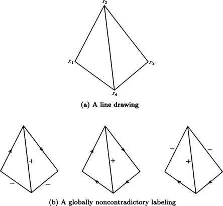
[1] Let X = {x1, x2, x3, x4}. The following is a list of possible labels for each vertex (Local labeling):
[2] None of L(xi) are empty. (Termination condition)
[3] Set the value of f(xi, μj) to 1 or 0. (Setting the initial value of the labeling function f)
[4] Pick the vertex x1 ∈ X arbitrarily. (Setting the starting point for one relaxation cycle)
[5] For the vertices x2,x4 that are neighbors of x1 (Starting the relaxation cycle),
Thus, set f (x1, angle < <) = 0. Similarly, set f (x1, angle < +) =0 Also,
So, set f (x1, angle+<) = 0. As a result, we find that we cannot assign the label angle<<, angle <+, or angle+< to the vertex x1.
[6] Let X = {x2,x3,x4}. (Ending the relaxation cycle)
[7] If ![]() go to [4]. (Condition for terminating one relaxation cycle)
go to [4]. (Condition for terminating one relaxation cycle)
[4] Select the vertex x2 ∈ X arbitrarily. (Setting the starting point of one relaxation cycle)
[5] For the vertices x1,x3 that are neighbors of x2 (Starting the relaxation cycle),
Since there is no pair y ∈ {x1,x3} and μk ∈ L(x2) that makes g(x2,y,μk, μ) = 0 for all of those labels μ making the value of f 1, no label can be found that can be assigned to x2.
[6] Set X = {x3,x4}. (Ending the relaxation cycle)
[7] Since ![]() , go to [4]. (Condition for terminating one relaxation cycle)
, go to [4]. (Condition for terminating one relaxation cycle)
[4] Select the vertex x3 ∈ X. (Setting the starting point of one relaxation cycle)
[5] For the vertices x2,x4 that are neighbors of x3 (Starting the relaxation cycle),
and for all μ ∈ L(x3),
So set f(x3, angle>+) = 0. Similarly, set f(x3, angle>>) = 0. Thus we find that the vertex x3 cannot be labeled by either angle>+ or angle>>.
[6] Set X = {x4}. (Ending the relaxation cycle)
[7] Since ![]() , go to [4]. (Condition for terminating one relaxation cycle)
, go to [4]. (Condition for terminating one relaxation cycle)
[4] Select the vertex x4 ∈ X. (Setting the starting point of one relaxation cycle)
[5] For the vertices x3,x1 that are neighbors of x4 (Starting the relaxation cycle),
and for any μ ∈ {angle+ >, angle < −, angle <<, angle- <}
So, set f (x4, fork +-+) = 0 In other words, the vertex x4 cannot be labeled by fork +-+.
[6] Set ![]() . (Ending the relaxation cycle)
. (Ending the relaxation cycle)
[7] Since ![]() , stop. The possible labels for each vertex are the following (Condition for terminating one relaxation cycle):
, stop. The possible labels for each vertex are the following (Condition for terminating one relaxation cycle):
In this way, we have obtained all the possible labelings. Prom these labelings, we can construct 3 × 3 × 3 × 2 = 54 possible combinations of global labeling for the four vertices. However, they might include combinations of labeling that are globally inconsistent. For this reason, we need to check each of the 54 combinations for global inconsistency.
When we check, we find that the three combinations shown in Figure 5.9(b) are the only ones that are not globally inconsistent. As we saw, we need to enumerate for global inconsistency, but we can reduce a large number of inconsistent combinations by the discrete relaxation method above. In our example, the number of possible labels for each vertex is 6,3,6,3, respectively, so there are 6 × 3 × 6 × 3 = 324 possibilities. The above method reduced the number to 54. As a pattern becomes more complex, the relaxation method usually becomes more effective.
(d) The stochastic relaxation method
Suppose we have a set of features, X, extracted from a pattern and a set of possible labels, M. For any xi,xj ∈ X, μk,μl ∈ M, let p(xi, μk xj,μl) be the probability that the label of xj is μl and the label of xi is μk. For p(xi, μk|xj, μl), the following holds: For any xi, xj, μl
p(xi,μk)|xj, μl) can be thought of as the extent to which labeling xi with μk and xj with μl does not contribute to an inconsistent labeling, so it can be considered as a stochastic parameter that represents the compatibility of labels.
Below we assume, either statistically or from previous knowledge, that the value of p(xi,μk|xj, μl) is given for all xi, xj ∈ X, μk,μl ∈ M. In this case, we can use the following algorithm:
Algorithm 5.2
(the stochastic relaxation method)
[1] Set n = 0. (Initialization of the iteration)
[2] For iteration n, from the probability, Pn(xi, μ), that the label μ ∈ M is a label for each feature xi ∈ X, obtain the probability vector for a labeling, Pn(xi) = (pn(xi,μ1), …, pn(pn(xi,μm)). (Computation of the probability vector)
[3] Using the following formula, compute Pn+1(xi) = (pn+1(xi,μ1),…, pn+1(xi,μm)). (Updating the probability vector)
[4] Stop if ||Pn(xi)|| ≈ ||Pn+1(xi)|| for all xi ∈ X. If ![]() selectμ κi as the label for xi. Otherwise, go to [5]. (Termination condition)
selectμ κi as the label for xi. Otherwise, go to [5]. (Termination condition)
[5] Let n = n + 1 and go to [3]. (Repeating the iteration)
In Algorithm 5.2, γij represents the degree to which the label μl contributes to xj in the change of the labeling probability p(xi,μk).
Updating the probability vector ([3] in Algorithm 5.2), in an actual problem, consists of repeating the multiplication of the matrix whose elements are γijp(xi, μk|xj, μl) and the vector Pn(xj). Thus efficient parallel computation is possible. The convergence of this process is not generally guaranteed, but if the matrix (linear operator for relaxation method) satisfies appropriate conditions, it can be proved to converge globally, that is, independent of the initial value of the probability vector P0(xi) (xi ∈ X).
This method can be used for matching a pattern with noise or other defects because it treats the labeling as a probability distribution. Since, like the discrete relaxation method, it is based on only the local compatibility of the labeling, it does not always result in a globally consistent labeling. It still requires a test of global consistency of the labeling.
(e) Graph matching and its evaluation measure
Results from the relaxation method can easily be represented by graphs. Also, if we use graphs to represent knowledge for pattern understanding, such as semantic networks, we can generally make the amount of memory needed small. As a result, graph matching methods become important for matching two patterns or for matching a pattern against such knowledge.
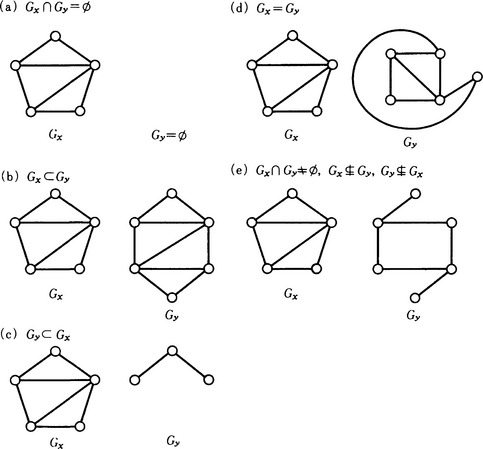
First, let us consider evaluation measures for matching. Matching two graphs can be divided into three cases as in Figure 5.10: when they completely match, when they do not match, and when they partially match. Of these cases, partial matching is important here, because in pattern understanding graphs corresponding to two patterns will usually only partially match.
In partial matching, there are two problems:
(i) We need to evaluate the similarity of two graphs.
(ii) The computing time for such matching algorithms increases exponentially with the size of the graph (for example, with the sum of the numbers of nodes and edges).
Here, let us consider (i), the evaluation measure.
Suppose two patterns X and Y are represented by two directed graphs Gx and Gy. Let Vx and Vy be the sets of nodes of Gx and Gy, respectively, and suppose the elements of Vx and Vy correspond to some features, like vertices, boundaries, and regions, of X and Y. Also, let Ex and Ey be the sets of (directed) edges of Gx and Gy, respectively, and suppose the elements of Ex and Ey correspond to relations between two features of X or Y.
First, let us consider an evaluation measure for the similarity of two graphs. When the names of the nodes of two directed graphs Gx and Gy are appropriately overlapped, we can express the degree of similarity using O = |V| + |E| where |V| is the number of overlapping nodes and |E| is the number of overlapping edges.
For example, five kinds of overlapping for the graphs Gx and Gy are, as shown in Figure 5.10,
The values of O for (a)-(d) are, if we take the names of the nodes appropriately, |Vx| + |Ex|, |Vy| + |Ey|, |Vx| + |Ex|, respectively. For (e), the value satisfies 0 < O < min {|Vx + |Ex|,|Vy| + |Ey|}.
The measure O can be thought of as one measure of the size of the maximum subgraph isomorphism of two graphs.
An algorithm that finds a subgraph isomorphism with the largest O (in other words, the maximum subgraph isomorphism) for two directed graphs X and Y basically has to check every possible pair of subgraphs. Improving the efficiency of such an algorithm requires heuristic knowledge. For example, in pattern understanding, a node of a graph usually corresponds to a feature, to which at tribute-values such as texture and color are often provided. In a graph, these attribute-value pairs may be represented by a self-loop at a node. We can introduce the heuristic knowledge that, when matching two patterns, features need to have the same attribute-value pairs, represented by the self-loops, in order to match. Then we can limit the search for a subgraph isomorphism to nodes whose self-loop labels are the same. This can reduce the time needed for the search.
If we only want to find such a graph with the locally largest value of O, that is, a locally maximal subgraph isomorphism rather than the globally maximum subgraph isomorphism, we may possibly find a solution in a short time. However, the graph search usually attains many local maxima, and there is no guarantee that a local maximum value of the evaluation measure is close to the global maximum.
5.3 Maximal Subgraph Isomorphism and Clique Method
In this section we will explain a method from graph theory that provides an algorithm for obtaining a maximal subgraph isomorphism of two labeled directed graphs. This method can easily be applied to a graph without labels. First, let us consider the labeled directed graphs Gx = (Vx, Ex, Cx), Gy = (Vy, Ey,Cy), where Cx and Cy are the sets of labels of the edges of Gx,Gy, respectively. We define the association graph of Gx and Gy as follows:
Definition 1
(association graph) Suppose two labeled directed graphs ![]() and
and ![]() are given. For
are given. For ![]() , Let
, Let ![]() and
and ![]() , and
, and ![]() . The undirected graph A (S,U) is called the association graph for Gx and Gy.
. The undirected graph A (S,U) is called the association graph for Gx and Gy.
In this definition, it is possible to restrict the elements in the set E using heuristic knowledge. For example, as we noted in Section 5.2(e), it is possible to define E by only collecting pairs of nodes representing features with the same attribute-value pairs.
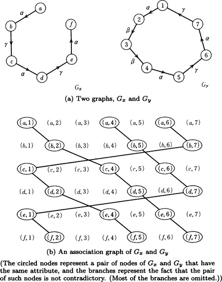
Now, a maximal subgraph isomorphism of two graphs Gx and Gy corresponds to a maximum clique of the association graph for Gx and Gy. For example, let us consider the two graphs shown in Figure 5.11(a). Their association graph G is shown in Figure 5.11(b). There are three maximum cliques in G, each shown as a solid line. (In order to make the illustration simpler, we did not show most of the edges.) Each of these corresponds to a maximal subgraph isomorphism.
From these, we can formulate the following algorithm for detecting the maximum cliques of the association graph as a method for finding maximal subgraph isomorphisms of two given graphs.
Algorithm 5.3
(detecting maximum cliques for finding maximal subgraph isomorphisms)
• Suppose there is a procedure C(H, K) that takes as inputs H = (Vh, Eh), a clique of the graph G, and K = (Vk, Ek), a subgraph of G that includes the nodes of H, and outputs all the cliques included in K. In particular, ![]() returns all the cliques of G. C(H,K) can be defined recursively as follows:
returns all the cliques of G. C(H,K) can be defined recursively as follows:
(1) If for any v ∈ Vk − Vh there exists a v′ ∈ Vh such that (v, v′) ∉ Ek, then return H.
(2) Otherwise, there is a v* ∈ Vk such that (v*,v′) ∈ for all v′ ∈ Vh. Find v*. Then compute C(H*,K) ∪ C(H,K*), where H* is the graph obtained by adding the node v* and all the (v*,v) ∈ Ek (where v ∈ Vk − Vh) to H and K* is the graph that is obtained by deleting the node v* and all the (v*,v) ∈ Ek (where v ∈ Vk − Vh) from K.
[Detection of maximum cliques]
• In order to find a maximum clique, compute C(H*,K) ∪ C(H,K*) recursively in (2) for all possible v*.
As an example, suppose we obtained the two graphs shown in Figure 5.11(a) from the two patterns shown in Figure 5.12. The association graph for these two graphs is shown in Figure 5.11(b). If we use the above method [detection of maximum cliques], we find the three maximal cliques shown in Figure 5.11(b).
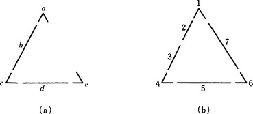
Figure 5.12 Patterns that yield the graphs Gx and Gy in Figure 5.11.
In this section we described methods of pattern matching using graph matching. These methods are clear and easy to see as they are based on the algorithms of graph theory. However, they are only for structures that are completely represented by graphs, so they are sometimes not so effective for patterns that include noise or defects.
5.4 Control in Pattern Understanding
To understand patterns, we need to combine many different processes. The efficiency of pattern understanding depends on how we control various processes. Also, there are many problems we have not yet covered, such as interpolating incomplete patterns based on knowledge, integrating processing of different levels, and so on.
In this section we will look at these problems from the viewpoint of control in pattern understanding.
(a) Bottom-up and top-down processing
First, as an example, let us look at the pattern of a “hammer” shown in Figure 5.3(a). Figure 1.5 shows the result of feature extraction from the pattern of a “hammer” other than the one in Figure 5.3(a). Furthermore, Figure 1.6 shows the result of matching knowledge against the extracted features.
Since matching algorithms do not usually look into the details of features, matching against knowledge does not always work correctly. Sometimes it results in a contradiction with past analysis. Therefore, an algorithm needs a flexible method of control that can use feature extraction and knowledge utilization alternatively. We can summarize this in the following conceptual algorithm:
Algorithm 5.4
(bidirectional control in pattern understanding)
[1] Let f(x) be a given pattern function.
[2] Do feature extraction on f(x) and let the result be g(x). Parts with more than one interpretation are left as they are.
[3] Match g(x) against our knowledge. If we do not find knowledge k that matches g(x) well, then stop. Output g(x). Otherwise, go to [4].
[4] Using inference based on k, make the incomplete or ambiguous (multiply interpreted) parts of g(x) more complete and call the result g(x) again. If the result is satisfactory, then stop. Output g(x). Otherwise, go to [2].
In Algorithm 5.4, [2] is called bottom-up processing or data-driven processing; [3] and [4] are called top-down processing or model-driven processing.
In pattern understanding based on knowledge, it would be ideal to perform bottom-up and top-down processing bidirectionally. However, we need to note that, since knowledge is generally incomplete, there is no general guarantee that the new pattern obtained in [4] gives a better result than previous iterations.
In Algorithm 5.4, bottom-up and top-down processing are executed in the following way:
Algorithm 5.5
[1] Preprocess the input data with techniques like the elimination of noise using smoothing.
[2] Extract local features of the pattern such as fragments of boundaries, small regions, color, or texture.
[3] Extract global features from local features.
[4] Generate a global representation of the pattern like a line drawing.
Algorithm 5.6
[1] Find a consistent labeling for the global features of the pattern.
[2] Match the labeled features against our knowledge.
[3] Interpolate the object’s representation based on the knowledge.
As an example, consider a pattern understanding system for finding a tumor in an X-ray photograph. First, bottom-up processing is used to extract features from a given X-ray photograph.
Next, if the system knows that tumors are likely to grow in a lung, it can try to find the outline of the lung and its inside from fragmentary features extracted from the X-ray photograph by top-down processing using knowledge of the structure of a lung.
On the other hand, even if the system obtained the outline of the lung, knowledge about where we might find a tumor in the lung does not exist. The system needs to narrow down candidates for a tumor using bottom-up processing.
Furthermore, in order to select the most likely candidate for a tumor, top-down processing using knowledge of the lung’s structure may be effective.
As in this example, a pattern understanding system can concentrate its attention on a selected candidate and analyze it in detail by controlling bottom-up and top-down processing bidirectionally. Also, at each point of processing it can combine appropriate methods of feature extraction and pattern matching.
(b) Interpolating representation based on knowledge
We now explain more concretely some methods of accomplishing the control described conceptually in (a). First, we describe a method for interpolating a representation based on knowledge.
Consider understanding the pattern of a polyhedron shown in Figure 5.13(a). We assume that we have obtained the boundary lines of the polyhedron as shown in Figure 5.13(b), using bottom-up processing.
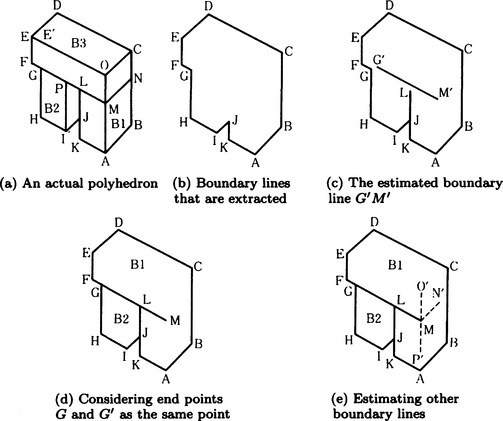
Figure 5.13 Interpolating representations using top-down processing with heuristic knowledge. (Shirai, 1975)
If we know the heuristic “When there is a concave angle on the boundary, each side of this angle becomes part of the boundary of different objects,” we can predict that there are boundary lines around the angles G and J and find new boundaries from fragmentary features around G and J. The result is shown in Figure 5.13(c).
Furthermore, if we use two other heuristics-“The end point of a boundary line connects to another boundary line” and “If two vertices are close each other, they are actually one vertex”-then we can interpolate the structures as shown in Figure 5.13(d) and (e) and can, in the end, obtain the structure shown in Figure 5.13(a).
(c) Control of modules using the blackboard model
Suppose we have several independent computation modules and one memory shared by those modules. A computing model for problem solving by repeated execution of modules, each of which gets its input from the memory and writes its results to the memory, is called the blackboard model
We now describe a method of control for pattern understanding using the blackboard model. As an example, let’s look at an understanding system for aerial photographs based on the blackboard model. Figure 5.14 shows a summary. This system has both a region extraction module and an object recognition module. The former analyzes the pattern spectrum, shape, texture, and so on to extract regions and writes them to memory. The latter takes regions found by the former from the memory and does further analysis to estimate larger regions.
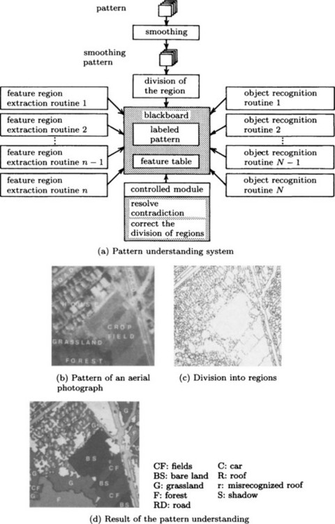
Figure 5.14 An understanding system and its analysis of an aerial photograph using the blackboard model. (Matsuyama and Nagao, 1980 (in Japanese))
The memory keeps such information as the density of features, threshold values, the directional angle of the sun, various values of attributes for regions, shapes of regions, labels for spatial relations, semantic networks representing conceptual relations among objects, and so on.
For pattern understanding, we can formulate, as independent computing modules, various algorithms for extracting features at various levels and algorithms for labeling and matching based on knowledge. Although the blackboard model is a cooperative computing system using multiple modules, each module is independent, so contradictory data can exist in memory at the same time. Also, information that may negatively affect problem solving can possibly be written out to memory.
In the control of the blackboard model, we need not only to schedule the priority to give to modules but also to resolve contradictions in the data and eliminate meaningless data. Therefore, a system based on a blackboard model often has, in the control module, a routine for finding and resolving contradictory data and a routine for correcting the estimated partition of regions.
(d) Constraint satisfaction by back constraint
When we try to match a representation obtained by feature extraction using bottom-up processing against knowledge, ambiguities frequently remain. For example, in the analysis of a photographic portrait using the generalized cylinder method, the length, L, and the direction, D, of a generalized cylinder are often hard to determine because the camera angle or the direction of the sun is often not clear. For such cases, we can represent knowledge using a set of inequalities like Lmin ≤ L ≤ Lmax, Dmin ≤ D ≤ Dmax as constraints.
Checking whether the length, L*, and the direction, D*, of a generalized cylinder obtained from feature extraction satisfy these inequalities or not corresponds to pattern matching. Furthermore, if L* and D* satisfy the inequalities, it is possible to estimate conditions when taking the photograph from the values of L* and D*. For instance, if knowledge of conditions when taking a photograph is represented as a set of inequalities about, for example, light rays in three-dimensional space, actual conditions for a given photograph can often be estimated by the values of L* and D*.
In this way, by propagating attributes of features satisfying constraints, we can often do consistent matching at various levels. This method is generally called constraint satisfaction by back constraint.
(e) Pattern understanding using production systems
By using production systems, we can often have flexible control over pattern understanding by combining declarative and procedural knowledge.
For example, we can keep a set of rules at each node of a semantic network and make them execute when the corresponding node is inferred. The scene understanding system described in Section 5.1(c)(4) is an example of a pattern understanding system based on a production system where the rules are localized.
There are two main differences between production systems and the blackboard model:
(1) Differences in modularization of knowledge
In a production system, procedural knowledge is represented by relatively small rules, and it is necessary to represent declarative knowledge of objects somewhere else, using frames, a semantic network, or some other declarative representation. In the blackboard model, we frequently use relatively large computing modules that join declarative and procedural knowledge together.
(2) Differences in inference method
In a production system, matching the condition side of a rule and the content of memory is the basic inference process. In the blackboard model, more complicated matching between a module and memory content is possible.
From these differences, we can say that a production system is useful for detailed control using a set of relatively small procedures, whereas the blackboard model is more appropriate when knowledge is too complicated to be divided into rules. However, in an actual problem, what kind of computing model is appropriate depends on the problem domain, and it is hard to determine what control method is best in general.
(f) Pattern understanding by plan generation
If we uniformly analyze every part of the pattern, it may sometimes take too much computing to find a specific object X in a pattern that includes many objects. It is convenient if we have some method of control for the priority we give to analyzing features of X.
Here, we consider plan generation as an example of this method of control. For example, in order to check, in a short amount of time, whether an aerial photograph of an airport includes a runway with a service road, we can execute the following procedure:
Procedure for plan generation
Generate the following plan to find a runway with a service road.
• goal: find a runway with a service road
• subgoal[1] Find a runway
[1.1] Find the convex hulls (a convex hull of a set of points is the minimum convex set including those points) of a set of sample points with some particular density, which approximates a region with a narrow belt shape.
• subgoal[2] Find a service road that crosses the runway.
In the above plan, subgoals [1] and [2] are AND goals. For a goal above those subgoals to be attained, both subgoals need to be accomplished. Subgoals [2.1] and [2.2] are SEQUENCE goals and need to be attained in that order. Furthermore, subgoal [1.1] needs to be accomplished before [2.2]. Also, since subgoals [1.1.1] and [2.1.1] are attained by the same procedure, it is sufficient if either one of them is accomplished.
Thus, the above plan has chronological constraints on subgoals and is generally called a nonlinear plan. If a system has enough information to generate a nonlinear plan like the example, it has the possibility of finding an object in a short time by paying attention only to the necessary parts of a complex pattern. Sometimes generating a plan itself requires complicated inference, so if plan generation is used to control pattern understanding, the computation time as a whole may not always be improved.
(g) Expert vision
As we continue to study control in pattern understanding, we realize that a system for pattern understanding basically consists of a set of modules with various kinds of technical knowledge and the interaction among such modules. This makes it possible to construct a support system that organizes these modules to make them easier to use and makes it possible for a user who is not a specialist in pattern understanding systems to do pattern understanding by combining modules in an appropriate way. A support system that functions like this is called an expert vision system.
The knowledge that a pattern understanding system needs is mainly divided into two kinds:
(1) Knowledge necessary for extracting features from a pattern and generating some representation.
(2) Knowledge for combining and controlling various methods for pattern understanding.
In an expert vision system, the latter knowledge is systematized and is used in applications to determine automatically what method to use for visual image processing and so on.
Summary
In this chapter, we described methods of understanding patterns using knowledge.
5.1. Pattern understanding is the generation, using knowledge, of a representation of what objects are included in a pattern, what are their attributes and values, and what are the relations among those objects.
5.2. Two important methods of knowledge representation used in pattern understanding are the superordinate/subordinate relation and the whole/part relation for classes of objects.
5.3. Symbolic representations such as semantic networks, frames, and rules can be used as knowledge representations for pattern understanding.
5.4. The relaxation method is a method for matching features extracted from a pattern against knowledge. Pattern understanding can use both the discrete relaxation method and the stochastic relaxation method.
5.5. If we represent, as graphs, the results of feature extraction and labeling by relaxation and represent knowledge also as graphs, graph matching algorithms become an important method for pattern understanding.
5.6. A maximal subgraph isomorphism of two labeled directed graphs can be obtained by finding a maximum clique in the association graph for the two graphs.
5.7. In order to control the process of pattern understanding, both bottom-up processing (data-driven processing) and top-down processing (model-driven processing) can be used.
5.8. The method of interpolating a representation based on heuristic knowledge can be used for top-down processing.
5.9. Control of computing modules using the blackboard model, constraint satisfaction using back constraint, and plan generation are methods of control in pattern understanding systems.
5.10. An expert vision system is a support system for performing pattern understanding by intelligently combining knowledge modules and control modules.
Exercises
5.1. Describe the difference between extracting features of a pattern and understanding a pattern. Also enumerate the information necessary for pattern understanding.
5.2. We say that two graphs G1 = (V1,E1) and G2 = (V2,E2) are graph isomorphic when there is a one-to-one correspondence between the elements of V1 and V2 and the elements of E1 and E2, and that this correspondence extends to any edges {v11,v12} ∈ E1, {v21,v22} ∈ E2 in corresponding nodes 〈 v11,v21〉 〈 v12,v22〉. Describe an algorithm for judging if two given graphs are graph isomorphic or not. Using this algorithm, show that the graphs given in Figure 5.10(d), Gx and Gy, are graph isomorphic.
5.3. In pattern understanding using plan generation, a set of subgoals that has the property that if any one of the subgoals is accomplished, we consider the set to be accomplished, are called OR goals. Show examples of pattern understanding where it is necessary to generate a plan including both OR goals and AND goals. Also describe an algorithm for plan generation including both OR goals and AND goals.
*A “triangle” is a concept. In order to describe our knowledge of an object declaratively, we need to consider how to describe the concept of the object. However, in this section, rather than discussing concepts in detail, we will assume that a set of characteristics common to instances of an object constitutes a concept. We will define the idea of a concept more clearly in Chapter 6.