
Business Simulation
Some business models can be simulated. Business process models can be simulated to determine costs, cycle times, and other process results. Business motivation models can be simulated to determine the results of strategies and trends. In either case, simulation is useful for training, persuasion, and analysis. Simulation is also useful for model validation—for finding and fixing errors in a model.
After the successful acquisition of the Cora Group, your management team at Mykonos entrusts you with a new responsibility: improving customer satisfaction across all the Mykonos restaurants. Traditionally Mykonos management has thought about customer satisfaction in terms of the quality of the dishes prepared, and part of your new job is to monitor the quality by traveling around the country and dining at Mykonos restaurants. But you believe that customer satisfaction at restaurants reflects other issues as well—issues that in the past Mykonos central management had ignored. You intend to use your new responsibility to consider customer satisfaction more broadly.
In particular you want to look at customer wait times and the impact of waits on satisfaction. At some of the more popular Mykonos restaurants, patrons wait. They wait for a table to be available. They wait for water, wine, and bread. They wait for the waitstaff to take their orders. They wait for their food, and they wait for their bills. You are concerned that all this waiting makes customers dissatisfied and hurts the success of these restaurants. And you suspect that some simple policy changes could reduce the waits and make the restaurants more successful.
But your focus on waiting is just a hunch, based on your experience of the restaurant business. You are not certain you are right. And even if you were certain, you face big communication and persuasion challenges. The general managers of the individual restaurants have a lot of independence. Each sets the policies for his restaurant. You are not sure how you can convince them to take action and reduce the customer wait times.
You ponder the situation for several weeks while working on other problems. Then you talk to a freelance restaurant consultant—Rhonda Martinez—to seek her advice about this problem. She suggests creating two simulation models. One model is focused on the customer dining process—how customers arrive, are seated, have their orders taken, and so on. The other model has a longer time scale. It is focused on customer satisfaction—how food quality, wait times, and other factors contribute to customer satisfaction and how word of mouth and restaurant reviews affect the view of potential customers and, ultimately, a restaurant’s success. She claims that these two models could serve to analyze the problem: to analyze wait times and the effect of wait times on customer satisfaction and restaurant success. Working with the models, she could examine the effect of different policies on wait times. And she claims that the two models could help communicate the results to the many restaurant general managers, ultimately persuading them to change their policies and reduce the wait times.
You have little experience with simulations yourself, beyond playing the simulation game SimCity. But you have worked with Rhonda before, and you have confidence in her work. You decide to try a simulation approach.
Why Simulate?
In Chapter 1 we describe the eight purposes for business models. Model simulation can address three of those eight: training and learning, persuasion and selling, and analysis.
Simulations have long been recognized as useful for training and learning. There are hundreds of commercial training games that use simulation. And some mass-market consumer entertainment simulation games are also used for training by universities. For example, the game Capitalism™ has been used in classes at Stanford School of Engineering and Harvard Business School. The use of simulations for training is a mainstream activity today.
But training with a commercial sim is inevitably a compromise; no commercial sim will exactly match the situation you want to teach. Usually there is no commercial sim that even comes close. Fortunately, custom simulations are a good training alternative when no commercial sim fits. A homegrown sim can be created to exactly match your purposes. As we show in this chapter, simulations are not difficult to build.
One of the reasons simulations are so effective for training and learning is that people find playing a simulation enjoyable. Whether homegrown or commercially purchased, simulations are fun.
The use of simulation for training is well-understood and widely appreciated. But simulation can also be a powerful tool for persuasion, and this use of simulation is not widely appreciated. In fact, simulations are used so rarely for persuasion that sims are something of a secret sales weapon—an advantage to the people and companies who make use of them.
B. J. Fogg, the director of the Stanford Persuasive Technology Lab, says, “Cause-and-effect simulations can be powerful persuaders. The power comes from the ability to explore cause-and-effect relationships without having to wait a long time to see the results and the ability to convey the effect in vivid and credible ways.” [Fogg 2003] Today when people want to persuade, they typically uses verbal techniques, numbers and graphs, or images and video. All these media have limited effectiveness. People dismiss words, ignore numbers, and are sophisticated critics of images and video. But simulations give them the ability to try things out, to experiment and build up their own understanding inside the simulated world. Simulations encourage people to reach their own conclusions through their own trial and error, but faster and more safely than they can in the real world.
As Fogg points out, simulations always come with a point of view. For example, in SimCity it is much easier to build an effective, prosperous metropolitan area if you design an extensive rail system. Will Wright, the creator of SimCity, is apparently a strong proponent of rails instead of roads and designed SimCity to reflect his point of view.
When persuading, you are attempting to communicate a point of view. Often you work against the ingrained biases of your audience. At Mykonos, the general managers of restaurants regard long customer waits as a good thing. The waits are a sign of the popularity of their restaurants and a symbol of their personal success. Convincing them that customer waits undermine their future success is difficult. Powerpoint presentations won’t be effective in changing their minds. You want them to try a restaurant simulation with that scenario. They can try to manage a popular restaurant with long lines, and see how poor customer satisfaction, bad restaurant reviews, and general ill-will erode the success, leading ultimately to closure.
Howard Gardner describes seven techniques for changing people’s minds: reason, research, resonance, redescriptions, rewards, real-world events, and resistances [Gardner 2004]. When well-designed, a simulation can play to three of these techniques. First, when someone plays a simulation, she becomes engaged. The simulation feels real to her, as though she is really (for example) a mayor of a city. The (simulated) real-world events change her mind. Second, a simulation provides an environment for someone to do (simulated) research by letting her try out experiments and seeing what happens. These experiments are in some ways better than real-world research because they can be performed quickly and without risk. Many alternatives can be tried out that would be expensive or impossible to try in the real world. Finally, a simulation is in its very essence a redescription, a different way to tell a story that can supplement a traditional pitch.
As personal experience, we have used business simulations in the sales pursuit of many large system integration projects. We have sold projects worth a total of several billion US dollars using simulation. Our personal experience is that simulations are strikingly effective in demonstrating a deep understanding of a customer’s problems, and convincing them that a proposed solution will solve those problems.
Simulations are also good for analysis. Chapter 10 describes several analysis techniques—ways of analyzing a model to reach conclusions about either the model or the business situation being modeled. Simulation can be used as an additional analysis method, a dynamic analysis method to complement the static methods of Chapter 10.
Why do we need another analysis method? For larger models, there are many questions that are too difficult to answer via static analysis. For example, with a small and simple business process model, it might be possible to analyze the cost of the end-to-end process using static analysis without simulation. But most processes are not small and simple. Most have many activities, and the more activities a process has, the more difficult it is to analyze statically. Most processes are complex, with uncertainty, intermittent resource constraints, and cyclic behavior. Complex processes are very difficult to analyze statically. Simulation is required for all but the smallest and simplest business processes.
Motivation models have the same characteristics. Small and simple motivation models can be analyzed statically to determine how the goals, strategies, and influences will lead to results. But most motivation models are neither small nor simple. They have many interacting elements, and they have feedback, time delays, and uncertainty. For these larger and more complex motivation models, simulation is the only effective method of understanding what will happen.
Simulating a Business Process Model
Rhonda starts by creating a simulation of the business process, to analyze and understand the causes of the customer waits. She intends to build a general model of restaurant waits that can be adapted to any of the Mykonos restaurants, but she doesn’t start by creating something general. Instead she starts by creating a model that replicates the ebb and flow of a single restaurant, Zona.
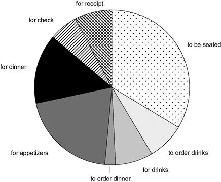
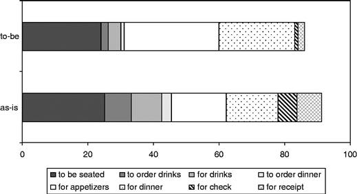
After some one-on-one modeling sessions with the Zona general manager and some observations of the restaurant in action, Rhonda creates a business process simulation. The simulation shows that each customer party waits 46 minutes on average. This 46 minutes includes all the waits: waiting for a table, waiting for a server to take their order, waiting for their dinner, waiting for their check, and waiting for their change or credit card receipt. The 46 minutes excludes the time spent considering the menu, ordering food and drinks, eating, and settling the bill. Figure 11.1 shows an initial simulation result, a breakdown of the average times spent by customers, organized by activity and presented as a pie chart.
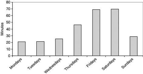
Wait times vary over the course of the week. Mondays and Tuesdays see far fewer customers than Fridays and Saturdays, and far shorter waits. The model has accounted for the typical number of customers on each day and when those customers arrive. The simulation produces wait times by day of the week, as shown in Figure 11.2.
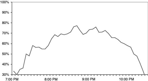
Wait times also vary over the course of a single evening. The wait times are shortest both early and late in the evening and longest in the middle of the evening, when the restaurant is busiest. Figure 11.3 shows a third simulation result: how the wait times vary over the course of a single Friday evening. Here, instead of an average wait time, the simulated waits are expressed as a percentage. Of all the customer parties in the restaurant at 8:30 PM, what percentage are waiting for something: for a table, for dinner, for their check? Similarly, at 8:40 PM, what percentage are waiting?
The simulation results in Figures 11.1, 11.2, and 11.3 are not intended to create any analytical insights—not yet. So far Rhonda has only replicated the current as-is situation at Zona. The simulation results validate that the model is reasonably accurate, that the model reflects the actual wait dynamics at the Zona restaurant.
Now Rhonda turns to analysis. She starts with a simple experiment. What happens if the staffing is doubled? What happens on Friday nights if there are two hosts available to greet and seat customers instead of one, twice as many servers waiting tables, twice as many chefs cooking meals, and twice as many bartenders mixing drinks? This is clearly an unrealistic experiment—Zona is not going to double their labor costs just to reduce customer wait times. But it is a revealing experiment. Are the customer waits due to staffing resource or due to some other cause?
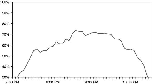
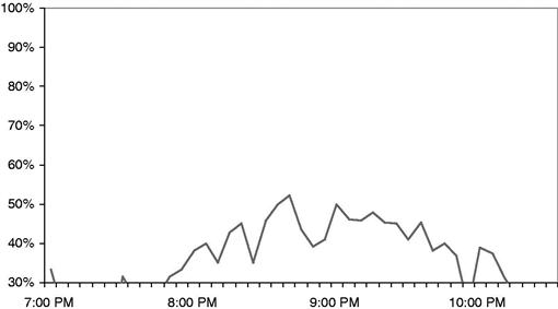
Figure 11.4 shows one of the results of the experiment—the percentage waiting through the course of a Friday evening. Figure 11.4 is directly comparable to Figure 11.3. The only difference is the staffing of the simulated restaurant. As you can see, there are some declines in wait times, but only modest reductions. At its worst, the Friday night waits with twice the staff are almost 90 percent of the current waits.
Why is the reduction in wait times so modest even when the staff is doubled? Rhonda analyzes the difference by looking at a single simulated party of four in both the as-is model and the (unrealistic) to-be. Figure 11.5 compares the breakdown of wait time for a single party arriving at the peak of Friday evening. On the bottom is the breakdown of waits for the party of four in the as-is model. On the top is the breakdown of waits for the party in the to-be model. The to-be party waits almost as long as the as-is party, but they wait at different points in the process. Instead of waiting for their bill to be prepared or for their server to take their order, their wait is concentrated at two points: waiting for a table and waiting for their dinner. By doubling the staff, we have succeeding only in shifting the wait time.
Of course, if every table is already occupied, a newly arriving party cannot be seated. They must wait for someone to leave. And when a party orders dinner, the food cannot be prepared if the kitchen capacity is fully taken by other dinners cooking. So Rhonda tries another experiment to test whether the tables and the kitchen capacity are creating the waits. In addition to doubling Zona staff, she doubles the size of the restaurant: the number of tables and the capacity of the kitchen. This is also unrealistic: Mykonos is planning no expansion in the size of Zona.
Figure 11.6 shows the Friday night waits for this double-size Zona. Most of the waits have disappeared. Customers still wait—of course they must still wait for their food to be prepared—but some of the waiting has been eliminated.
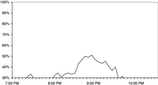
Figure 11.6 Percentage of customers waiting on Friday, with twice the staff, twice the tables, and twice the kitchen
Rhonda draws the obvious conclusion from this latest experiment: Zona is just not big enough for the demand on busy nights. Now it is time to try a realistic experiment. Suppose Zona changed their policy and only seated people with reservations on those busy nights. What if they eliminated waiting lists for tables? Rhonda models that policy change experiment. She first returns the model to the normal staffing and the normal size and then alters the process to turn people away who do not have reservations on Fridays and Saturdays. The results are shown in Figure 11.7. People are in fact waiting less. But that reduced wait comes at a cost: Zona is serving fewer people and the bar is serving far fewer drinks to people who are waiting.
Many other experiments are possible. What if Zona limited the size of the waiting list to allow no more than three parties to wait at a time? What if Zona staffed a single additional server on Fridays and Saturdays? What if Zona cross-trained the servers, so they could perform as hosts if the host was busy seating people? What if Zona only seated smaller parties—those of six people or fewer? All of these simulations could be modeled and the results examined.
You are planning to use the simulation to analyze different policies and improve your own understanding. But the wait times and changes in policy to reduce those wait times are ultimately the responsibility of the general managers of the individual restaurants. You intend to provide this simulation to those restaurant general managers so that they can experiment with various policies for their own restaurants.
Activities, Resources, and Jobs
What does it take to create the kind of business process simulation described in the last few pages? Of course you need a business process simulation engine, a software application that simulates the model. Often such an engine is included as part of a business process modeling tool.
You also need a good business process model, the kind of model described in Chapter 5. And you need to prepare that model to be run in a simulation engine. Preparing a model for simulation requires some additional work beyond what is required to create a static, non-simulated model. But more significantly than the extra work, preparing a process model to be simulated requires additional knowledge.
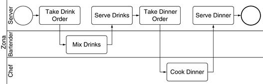
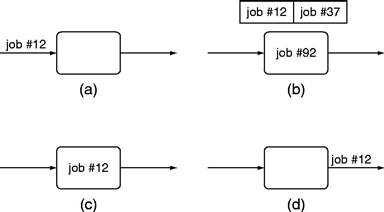
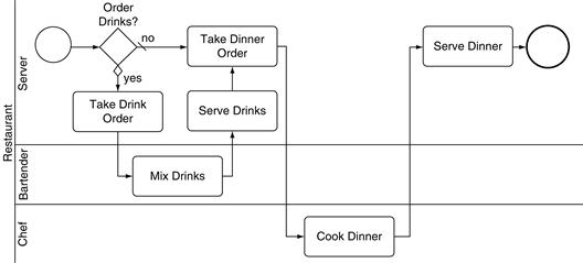
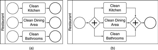
To create a business process simulation you must understand activities, resources, and jobs and the way these three interact with each other. As described in Chapter 5, a business process activity is a single step in a larger business process. In our model of customers dining at Zona (shown again in Figure 11.81), Mix Drinks is one activity and Take Dinner Order is another.
A resource is a person who performs the activity. The resource is identified in a business process by the swimlane where the activity is placed. For the activity Take Dinner Order, the resource is a Server. Note that the resource is an actual (simulated) person, whereas Server is a role the person plays. At any one time, many people will be playing the role of servers; seven different servers will be working on a typical Friday night. And over the course of an evening, one person may play multiple roles.
A job2 is something that flows through the process, being worked on by resources and flowing from activity to activity. Examples of jobs include a purchase order and a help desk trouble ticket. In our model of restaurant dining, each job is a customer party. Some jobs represent parties of two diners, some represent parties of four, some represent people dining alone.
The Job Cycle
A job is created at a start event and flows over sequence flows and message flows from activity to activity until an end event is reached. When a job reaches an activity, one of two things can happen. Either a resource is available to work the job or no resource is available and the job must wait until a resource is available, perhaps waiting in a long line of other jobs. Consider the activity Mix Drinks in Figure 11.8. The job arrives at this activity after the activity Take Drink Order occurs; after the party has ordered their drinks, the drinks can be mixed. At this point any bartender can mix the drinks. If a bartender resource is available, the activity can be performed. Otherwise the job must wait until some bartender is available.
Once a bartender is available, he performs this activity—mixing the drinks—until the activity is finished. While he is performing this activity he is not available to do anything else. He can neither mix other drinks nor perform other activities in the model. When he is finished mixing the drinks, the job and the resource separate. The resource is available to do something else—he can mix drinks for someone else or wash glasses or calculate someone’s bar tab. Meanwhile the job traverses the sequence flow to the next activity, Serve Drinks.
The job cycle is illustrated in Figure 11.9.
a A job arrives at an activity from the incoming sequence flow.
b It waits, perhaps behind a line of other jobs, for a resource to be available.
c Once the appropriate resource is available, the resource works the job.
d When finished with that activity, the job travels across the outgoing sequence flows to the next activity.
A business process simulation engine performs the job cycle thousands of times, every time a job leaves one activity and travels to another. The jobs—restaurant parties in our example—progress across sequence flows from activity to activity, progressing from Serve Drinks to Take Dinner Order to Cook Dinner. The resources—servers, hosts, and chefs in our example—work jobs when they are at activities.
Collecting Statistics
The simulation engine collects individual statistics as the simulation progresses—statistics about activities, resources, and jobs. These statistics are aggregated into the simulation results. For example, the results shown in Figures 11.1 through 11.7 are aggregated from thousands of individual statistics.
The engine collects statistics on each activity, each resource, and each job. Activity statistics include how many times each activity was performed, the average duration of each activity, the total cost of each activity, and the other activity statistics shown in Table 11.1. Resource statistics include the utilization of each resource, the total amount of work performed by each resource, and the other resource statistics shown in Table 11.1. Job statistics include the total cycle time of each job, the total touch time of each job, and the other job statistics in Table 11.1.
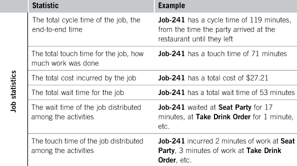
Statistics are collected for each activity, each resource, and each job, but these individual statistics are rarely examined by themselves. Instead they are aggregated in various ways, producing various averages and distributions. For example, each job keeps track of its end-to-end cycle time as it progresses through the process. When a job reaches an end event and finishes, the simulation combines that newly finished cycle time with others that have already finished and produces an average. It may also keep track of some other cycle time aggregates: how the average changes over the course of the simulation, the standard deviation of the cycle times, and how the cycle time varies with the type of job.
Activity Durations
To be simulated, activities need additional attributes. Duration is one such attribute. When a job arrives at an activity, how long does the resource work on it? Each activity has a duration attribute that indicates how long jobs need to be worked. Often that duration is a constant value, such as 10 minutes for every job that is worked by this activity. But duration can also vary, and it can vary in three different ways.
First, the duration can vary depending on the details of the job. For example, the Take Dinner Order activity takes much longer for a party of eight than it does a party of two. In fact, the party of eight takes longer for many activities in the customer dining process; not only does the activity Take Dinner Order require a longer duration for the party of eight, but so does Serve Dinner.
The job that models the party of eight needs to be different from the job that models a party of two. For this simulation, jobs need their own model-custom attribute, partySize. A job representing a party of eight will have a party size value of 8, and a job representing a party of two will have a value of 2.
Second, the duration of the activity can vary depending on the details of the resource. A skilled server will serve drinks quicker than a novice because she remembers who ordered which drink. The simulation needs to know that this server is quick, that one is average, and this other one is slow.
For this model, resources need a model-custom attribute, skillLevel, to keep track of skill. Values of skill level can then be 1 for an average skill, 0.8 for a quick server, and 1.2 for a slow one.
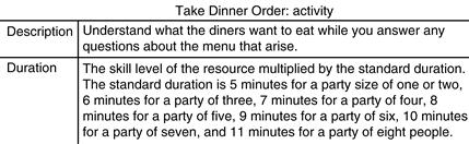
Suppose we want the duration of Take Dinner Order to consider both the skill of the server and the size of the party. How do we combine those elements? We need to encode the duration as a formula, perhaps like the duration in Figure 11.10. The standard duration depends on the party size: 5 minutes for parties of one or two, 6 minutes for parties of three, and so on. That standard duration is multiplied by the skill level of the server—multiplied by 1 for an average server, by 0.8 for a quick server, and by 1.2 for a slow one. (There is no standard technical language for encoding activity durations. In practice each BPMN tool that supports simulation has its own language. In this book we use precise English because our focus is not on the syntax of any language but on what needs to be expressed.)
Third, the duration of the activity can vary randomly. Consider the activity Cook Dinner. The duration of Cook Dinner might vary from 20 minutes to 45 minutes, depending on what is ordered.3 Sometimes it takes 22 minutes, sometimes 37 minutes, sometimes 41. As the simulation runs and Cook Dinner is executed for different jobs, each job takes a different duration, a random time between 20 and 45 minutes.
When durations vary randomly, modelers often employ a uniform distribution. Each duration in a uniform distribution within the range is equally likely; 20 minutes is just as likely as 33 minutes and just as likely as 40 or 45. Uniform distributions are easy for subject matter experts (SMEs) to understand.
It is also possible to use other distributions: a triangular distribution that peaks somewhere in the middle, a standard (bell curve) distribution, or something more sophisticated. Figure 11.11 shows some of the distribution alternatives.
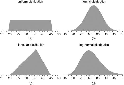
In practice, uniform and triangular distributions are commonly used, and the more complex statistical distributions are much more rare. The statistical distributions (e.g., normal, log-normal, exponential, etc.) often lead to higher model fidelity, but they are usually difficult for SMEs to understand. This is the modeling tradeoff between fidelity and simplicity, a tradeoff we have seen many times in this book.
Work Time and Delay Time
The duration of an activity specifies the work time—the time a person is actually working on a job. But a job can also experience a delay while it is at an activity, time when no one is actually working on the job. A resource delay occurs when there is no resource available to work a job. Consider again the job cycle shown in Figure 11.9. At step b, the newly arrived job waits for a resource to be available, perhaps in a queue of other jobs that are also waiting for resources. Step b is not work time, not part of the duration of the activity. Instead step b is resource delay time.
So a job can experience resource delay time while waiting for a person to start working it. A job can also experience resource delay after a person has started working it. The person working the job can become unavailable: she leaves for lunch, she takes a break, she goes home at the end of the day. When the resource working on a job becomes unavailable, the job experiences a resource delay.
In most situations this resource delay is a good approximation to what happens in the world being modeled: the work waits on the person’s desk until she returns to it after lunch. But sometimes in the real world, the work will not wait for the person working it. When a server in Zona leaves for the evening, if she has any remaining customers she will transfer those customers to someone else rather than making them wait until she returns the next day! But how does the simulation know that in this situation, customers are to be transferred to another resource? We use the resourceShift attribute of the activity: resourceShift indicates that the job should be given to another resource if the original one becomes unavailable. If resourceShift is false for an activity, a job at that activity can experience a resource delay even when there are available resources—for example, if the resource working the job at the activity leaves for the evening. If resourceShift is true for an activity, there will never be a resource delay there as long as at least one resource is available.
A job can also experience a resource delay before work has started. Suppose a job is waiting at the activity Collect Payment in our restaurant dining process of Figure 11.8; the dinner has been finished and the party is waiting for their server to settle the bill. Their server is busy with another table, so they wait for her, even though other waitstaff are available. The availability of other waitstaff does not matter; they need their server, the one who served them drinks and dinner and who has their bill. The job waits until that particular resource is available. The activity attribute consistentResource is used to indicate this situation—that the resource should be the same as the one used at the prior activity.
In addition to resource delays—waiting for a resource to be available—a job can experience an intrinsic delay. An intrinsic delay is a delay that occurs as part of the normal work of the job. Consider the activity Cook Dinner, when the chef is preparing food for the diners. There is much work in that activity, of course, but there are also times during the food preparation when the duck is grilling or the onions are sautéing and the chef is not doing anything on this dinner. He is either working on other dinners for other parties, or if the restaurant is empty, he just waits for the duck to be grilled. It might take 40 minutes to prepare the dinner: 25 minutes of work and 15 minutes of intrinsic delay.
When working a single activity, a job can experience both a resource delay and an intrinsic delay. Cook Dinner includes an intrinsic delay as part of the nature of preparing food. If many dinner orders arrive at once, the chef might have more work than he can do, and some of the dinners suffer delays—resource delays—until the others are finished. (Or as explained later in the chapter, the chef could be limited by the physical resources of the kitchen—if for example all the grills are occupied.)
Intrinsic delays and resource delays are both delays. In both situations, the job is waiting and no work is being performed. But they are modeled differently. If an activity has an intrinsic delay, its intrinsicDelay attribute will indicate the amount of time that the job is delayed. Resource delay is not specified in an activity attribute. Instead it happens when the process is simulated, as a job waits for a resource to work it.
A delay can also occur in a flow, either in a sequence flow between activities in the same pool or in a message flow between pools. For example, when a vineyard supplier to Mykonos submits an invoice for wine, that message flow might be implemented by physical mail, including a three-day delay for the US Postal Service to deliver the letter. For a simulation, a flow delay is like an intrinsic delay in an activity: the job just waits for the specified time and then continues.
Simulating Exclusive Gateways
As you may recall from Chapter 5, a gateway is used to model branching behavior when there are several different sequence flows a job can take and a decision is made about which one (or which ones) to take. Consider the process shown in Figure 11.12, a variation of the dining process of Figure 11.8. Sometimes diners do not order drinks before dinner. The gateway Order Drinks? has two outgoing sequence flows: one if the diners order drinks and another if they do not. Order Drinks? is an exclusive gateway; either drinks are ordered or they are not.
In the midst of a simulation, when a job arrives at an exclusive gateway, how does the simulation engine decide which way to send the job? Does this job represent a party that is ordering drinks or one that will move straight to ordering dinner? How do we model the exclusive gateway so that the simulation engine knows what to do?
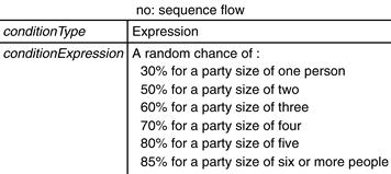
There are three alternative modeling approaches to this question. The simplest approach is for each of the outgoing sequence flows from the gateway to indicate a percentage of jobs. Each sequence flow has a conditionExpression attribute indicating whether the sequence flow will be taken. One of the sequence flows is a default; it is the flow taken if none of the others is chosen.
For example, suppose 60 percent of the parties order drinks before dinner and 40 percent do not. The lower sequence flow—connecting Order Drinks? to Take Drink Order—has a condition expression value of “A random chance of 60%,” indicating a 60 percent chance of taking that path. (As with durations of activities, there is no standard language for condition expressions. Each simulation tool supports its own language. We use a precise form of English in this book.) The upper sequence flow—connecting Order Drinks? to Take Dinner Order—is the default sequence flow. It is taken in the other 40 percent of situations.
A job that arrives at the gateway will have a 60 percent chance of taking the lower path and a 40 percent chance of taking the upper path. Each job is evaluated differently, so in the midst of a simulation run, it is possible for four jobs in succession to beat the odds and all take the upper path. But over the course of hundreds of jobs, the actual results will be close to 60/40.4
A second way of modeling how an exclusive gateway determines the outgoing path is to examine an attribute of the job. Suppose that each job in this model had a beforeDinnerDrink attribute, indicating whether the party will order drinks before dinner. For some of the jobs this attribute is true and for others it is false. Then for each job, the outgoing sequence flows from Order Drinks? will examine the value of this attribute. Those with a value of false will be sent along the upper path, and those with a value of true will be sent on the lower path.
Of course, this just pushes the problem from the sequence flows to the job. How does a job get a value for beforeDinnerDrink? In the process shown in Figure 11.12, a natural approach would be to assign this attribute in the original start event when the job is created. Perhaps 60 percent of the parties arriving would be drinkers, and those jobs would be given true values for beforeDinnerDrink as they are created. The other 40 percent would be given false values.
There are two advantages of driving a gateway using a job attribute instead of probabilities evaluated on the sequence flow.
1 Job statistics can be analyzed and sorted by the job attribute. For example, do diners who order before-dinner drinks stay longer at the restaurant than those who do not? How much longer? Do they experience more delays or fewer? These questions can be answered by comparing the statistical results of jobs that have a true value for beforeDinnerDrink with those that have a false value.
2 Attribute-based scenarios can be created. Suppose a large trade show is expected in town. Trade show participants are known to be more likely to drink (and to drink more) than typical restaurant patrons. A simulation scenario can be run in which for a few days 80 percent of the customers order drinks before dinner. Do longer wait times result? Does the restaurant need to staff more servers, or more bartenders, or both?
There is also a third way to model an exclusive gateway: combining the two approaches and making the gateway split depend on both an attribute of the job and on a random percentage. For example, the larger the party, the more likely someone will want to order a drink before dinner. The gateway sequence flows can be driven by logic that specifies a different percentage for different party sizes. Figure 11.13 shows the conditionExpression attribute of the lower outgoing sequence flow from the Order Drinks? activity in Figure 11.12.
Simulating Other Gateways
Exclusive gateways are the most commonly used variety of gateway, but other varieties are also used. As you will recall from Chapter 5, a parallel gateway starts parallel work—two or more sequence flows that then progress at the same time, perhaps to be later joined back together by another parallel gateway.
Consider the process shown in Figure 11.14, a refinement of Figure 11.12 that provides more detail on the preparation of food, showing the appetizers, entrées, and desserts. Figure 11.14 is a subprocess, just the preparation and serving of the food, without the messy details of seating the party and settling the bill. (And of course Figure 11.14 is quite simple, e.g., it assumes the party orders desserts.)
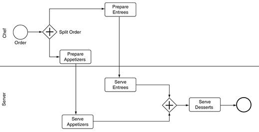
The chef starts the preparation of the appetizers and the entrées at the same time. The appetizers can be prepared quickly and are served to the customers when they are ready. The entrées take longer. When this part of the process is simulated, a single job will hit the gateway Split Order. The simulation engine splits the single job into two jobs, one traveling the upper sequence flow to Prepare Entrees and one traveling the lower sequence flow to Prepare Appetizers. Each of the two jobs collects statistics about the work—work time, delay time, etc.—as each progresses along its sequence flow. After the appetizers and entrées are served, the two jobs arrive at the other (unnamed) parallel gateway. At this point they are combined back into a single job, one that carries all the statistics of the two jobs that formed it.
Figure 11.14 assumes that each party orders both appetizers and entrées. An alternative approach is to use an inclusive gateway, as shown in Figure 11.15. In this case, a party can order just appetizers, just entrées, or both appetizers and entrées. During a simulation, the second (unnamed) gateway will do the right thing for each dining party. For a party that is eating both appetizers and entrées, the second gateway will wait for the two jobs to arrive before creating a new job from their combination. For a party that is eating only appetizers, the second gateway will pass the job through, not causing it to wait for anything. The analogous action occurs for the party that is eating only entrées: the second gateway will pass the job through.
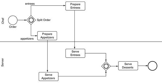
The behavior of the first gateway—Split Order—is a bit complex. When a job arrives at Split Order, sometimes the job needs to travel the upper path, sometimes the lower path, and sometimes it needs to be split so that the two parallel jobs can travel both paths. The logic is controlled by the conditionExpression attributes of the two outgoing sequence flows.
One approach to modeling Split Order is to encode the percentage of jobs that take each path. Perhaps 90 percent of parties order entrees, and 60 percent order appetizers, so the upper sequence flow might have a conditionExpression value of “A random chance of 90%” and the lower sequence flow one of “A random chance of 60%.” Since the two chances are independent, there are four combinations: 54 percent will order both entrees and appetizers, 36 percent will order entrees and no appetizers, 6 percent will order appetizers and no entrees, and 4 percent will order neither appetizers nor entrees.
This last 4 percent—in which neither path is taken—is a problem. An inclusive gateway needs to guarantee that at least one of the outgoing paths is taken or the model is considered invalid. But if condition expressions are used, 4 percent of the jobs will take neither outgoing sequence flow, leading to an invalid model.
Another, better approach that avoids the 4 percent problem is to generate the jobs with a custom attribute foodOrder that indicates whether the party orders appetizers, entrees, or both. Then the conditionExpression for the two outgoing sequence flows tests the value foodOrder of each job. The upper sequence flow tests whether foodOrder is either entrees or both, and the lower sequence flow tests whether foodOrder is either appetizers or both. Adding model-custom attributes to jobs is a useful technique that solves many modeling problems.
Simulating Start Events
Jobs are created at start events, travel through activities, gateways, and intermediate events, and finally finish their lives at end events. A start event typically creates many jobs, feeding a stream of jobs into a process. Consider again the restaurant dining process shown in Figure 11.12. The start event Party Arrives creates a job for each simulated party that arrives at the restaurant.
When does a start event create its jobs? Typically a start event will create some number of jobs every so often. For example, one start event might create two jobs every hour. Every hour of the simulation two new jobs are created. Another start event might create seven jobs every 20 minutes. Yet another start event might create one job every day. The Party Arrives start event in Figure 11.12 creates one job every 10 minutes; every 10 minutes a new party arrives at the restaurant to eat.
A start event has a jobQuantity attribute to model how many jobs are created at the same time and a jobInterval attribute to model the length of time between these times where jobs are created. Party Arrives in Figure 11.12 will have a jobQuantity value of 1 and a jobInterval value of 10 minutes.
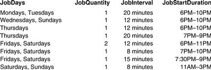
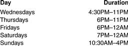
But things are a bit more complicated. Zona is not open all the time, only in the evenings. It doesn’t make sense for a new job to be created at 3:30 AM. There is another attribute that models the fact that the start event should only create new jobs at certain times of the day: jobStartDuration. Zona has a value of “5PM–10PM” for jobStartDuration.5
Of course Zona sees more customers on a Saturday night than they do on a Monday night. And more people show up between 7:00 PM and 9:00 PM than do before 7:00 PM or after 9:00 PM. As we saw earlier in the chapter, it can be important to model this variation, to see how much worse the waits are on Friday at 8:30 PM than on Monday at 6:30 PM. To model this variation, each start event has not just a single value for Party Arrives and jobStartDuration but a schedule of values. For the Party Arrives start event at Zona, that schedule is shown in Figure 11.16. On Mondays and Tuesdays, there is a steady but slow stream of customers, with one job started every 20 minutes between 6:00 PM and 10:00 PM. On Wednesdays and Sundays, there are more customers, one job started every 12 minutes. On Thursdays there is a job started every 12 minutes between 6:00 PM and 10:00 PM, and there are some additional parties that show up between 7:00 PM and 9:00 PM—an additional job every 20 minutes during those busy hours. On Friday and Saturday evening, there is a base level of jobs started between 6:00 PM and 11:00 PM, two parties every 12 minutes, an additional job every 8 minutes between 7:00 PM and 10:00 PM, and a further additional job every 15 minutes between 7:30 PM and 9:00 PM. Saturdays and Sundays also see Zona open for lunch and so there are jobs that start between 11:00 AM and 3:00 PM.
The schedule in Figure 11.16 shows a party arriving at Zona every 12 minutes on Wednesdays. That regularity is also a simplification. In the real world, parties arrive sporadically. Sometimes 30 minutes passes and no one shows up. Sometimes three or four parties will arrive in a few minutes.
It can be important to capture that variability in your model. When two parties arrive at about the same time, the second party will wait for the host to seat the first party. That wait will never happen in your model if you have modeled parties arriving regularly every 12 minutes.
It is possible to model a variation in arrival times. Instead of a fixed jobInterval of 12 minutes, you can include a probability distribution, e.g., a uniform distribution from 1 to 23 minutes, a standard distribution that averages to 12 minutes, or some more complex distribution, such as the duration distributions discussed earlier and shown in Figure 11.11.
The jobQuantity can also vary statistically. This variance is convenient when you are modeling a process that has a large number of jobs. For example, in Figure 11.16 there is a line in the schedule for Friday nights that has two jobs starting every 12 minutes between 5:00 and 11:00 PM. Instead of two jobs, you might model that as a uniform distribution of 1 to 3 jobs. One third of the time one party arrives, one third of the time two parties, and one third of the time three parties arrive at the same time.
A schedule in a start event can support high model fidelity; it is possible to get very precise about the load of jobs and the way that load varies from day to day. Of course, there are diminishing returns to that fidelity. Often a start event modeled at a lower-fidelity will deliver as good results as a higher-fidelity approach.
As discussed earlier, the jobs in our restaurant simulation will have a partySize attribute, indicating the number of people in the party. The party size for the job influences how long activities take and influences the probabilities within gateways. This model-specific job attribute is set when the job is created at the start event Party Arrives. How does this work? The start event has a collection of assignments, as shown in Figure 11.17.
When a job is created at a start event, it is given values for every attribute in the assignments collection. A job created at Party Arrives will be given a value for the attribute partySize of a number between 1 and 8, and a value for beforeDinnerDrink, either true or false. These attribute values will be part of the job, carried with it through all its activities, until the job finishes at an end event.
Simulating End Events
A job finishes when it reaches an end event. As you may recall, each job carries statistical information with it as it travels from activity to activity. (Table 11.1 shows the statistics carried by a job.) When a job finishes, its statistical information is aggregated with the statistical information of the other jobs that have previously finished.
For example, each job carries a cycle time—the amount of simulated time since it was created at a start event. For our restaurant dining model, the cycle time will be the amount of time a dining party has been at the restaurant, starting with their arrival at the restaurant. When the job finishes, its cycle time is combined with the cycle times of other jobs that have already finished. Now we can determine the average cycle time: how long diners spend at the restaurant from beginning to end. We can watch for a maximum cycle time: what was the most time some party spent at the restaurant? We can relate cycle time to other information tracked by the job: does cycle time depend on the size of the party?
When you are developing a simulation, you might find that some jobs never finish. Of course some jobs simply haven’t finished yet. If you run the simulation longer, they will finish. But sometimes jobs are started but never reach an end event, no matter how long you simulate. This happens when you have errors and mistakes in your model. Certainly in the real world, it would be odd if a restaurant party arrived at Zona on Friday night and never left! Later in this chapter we describe how you can look at job counts at activities to validate your model, to find and correct the errors and mistakes.
Simulating Subprocesses
Not every start event creates jobs. A start event within a subprocess does not create any jobs on its own. Instead it indicates where the subprocess starts. Suppose you were simulating the (rather simple) process of creating a daily specials menu, shown in Figure 11.18. The start event Start Specials starts jobs, presumably one job each day. But the start event Begin Plan starts no jobs on its own. Instead it shows where jobs that have left the activity Determine Ingredient Availability should begin the embedded subprocess Plan Specials. For the simulation engine, start events serve these two distinct functions.
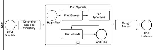
End events also serve two functions. The end event End Specials in Figure 11.18 finishes jobs. Any job that performs the activity Design Menus and then encounters End Specials will be finished at that point. Its statistics will be aggregated with the statistics of all the other jobs that have already finished. The end event End Plan is different. When a job hits that end event, it will finish the subprocess and travel across the sequence flow of the upper process, to Design Menus. Just as a start event in a subprocess does not create any jobs, an end event in a subprocess does not finish any. Of course, activity statistics are collected at each activity, including those that have subprocesses. But job statistics are not aggregated when a job hits a subprocess end event, since the job is not yet finished.
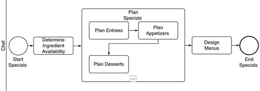
Often a subprocess will have neither a start event nor an end event. As explained in Chapter 5, if there is no start event in a subprocess, there is an implicit start event preceding each activity, event, or gateway that lacks an incoming sequence flow. In other words, Figure 11.19 (without start events) simulates just like Figure 11.18 (with start events). When a job finishes with the activity Determine Ingredient Availability, it drops down into the subprocess and starts the activity Plan Entrees, since that activity has no incoming sequence flow. It is as though there is an implicit start event before Plan Entrees, like the start event Begin Plan in Figure 11.18. When the job finishes Plan Entrees, Plan Appetizers, and Plan Desserts, it pops back up out of the Plan Specials subprocess and begins the activity Design Menus. It is as though there is an implicit end event after Plan Desserts, like End Plan in Figure 11.18.
Some subprocesses have multiple start events. Consider the subprocess with three start events shown in Figure 11.20a. When simulated, an incoming job will split and start the three start events in parallel. It is as though there is a single start event that leads to a parallel gateway; the subprocess in Figure 11.20a simulates exactly the same way as the one in Figure 11.20b.
Resource Schedules
People do not work all the time. Every person has hours he works and hours he does not work. To model realistic working times, resources have schedules. Just as a start event has a schedule for when jobs are created, each resource has a schedule for when he works. The schedule for a server who works at Zona is shown in Figure 11.21. As you can see, he works evenings Wednesday through Saturday as well as Sunday afternoons.
Resource schedules can be more detailed than shown in Figure 11.21. You can model breaks, holidays, vacations, and other HR detail. But often such detail is not useful. Many good models take a simpler approach. Rather than capture the schedule of each resource—each person—these simpler models just capture the schedule of each role. Figure 11.21 might be the schedule for the Server role, for all the servers in the model. This is another example of the tradeoff between the fidelity of more detail and the simplicity of less.
Resource Costs and Other Costs
Resources cost money. Most organizations pay more money for their human resources—their employees and contractors—than for any other expense. When a job simulates through a business process, the job accumulates the cost of each resource that works on the job. If a server spends 5 minutes serving dinner to a party, and the server costs the restaurant $12 per hour in costs, then $1 of costs will accumulate on the job that models that party.
To put the right cost on the job as it is worked by a resource, the modeler must capture the resource’s hourly cost. hourlyCost is another attribute of the resource. The hourly cost of each resource is captured separately because different people incur different hourly costs. Chefs are paid more than servers, who in turn are paid more than cleaning staff.
Hourly cost is not just the wages (or salaries) received by the employee. It includes the fully loaded cost to the employer of having the employee work: the cost of benefits, employment taxes, training, liability, etc. Sometimes the fully loaded cost for useful work is twice the wages or even more.
Some activities have other costs, in addition to the cost of the resource working the activity. For example, an activity that ships something across the country will incur the cost of the shipping service. This expense for the shipping service is in addition to the expense of the employee performing the shipping activity. The activity expense is captured in an attribute of the activity called additionalCost.
Nonhuman Resources and Multiple Resources
In most business process simulations, all the resources represent people. When a resource is working in a simulation, that resource represents a person working in the world. The schedule of a resource is a person’s schedule. The people-orientation of resources is not surprising: business process models are people-oriented. They model how people do work. Of course, when people work activities, they are often supported by machines—computers and software, production equipment, and the other artifacts of our technological age. But usually in business process models, we do not explicitly model the support machinery as resources. The availability of the machinery is usually not an issue; it is the availability of the people that constrains the work.
But we have already seen an exception, a situation where the modeling of nonhuman resources is important. In the customer wait model earlier in this chapter, the waits are caused partly by the limited number of tables. Consider again the process shown in Figure 11.12. A job at Seat Party will wait if there is no host available to seat the party represented by the job. But the job will also wait at Seat Party if there is a host available but no table. The activity Seat Party requires two resources, both a human resource—a host—and a nonhuman resource—a table.
An activity has an attribute resources that captures the resources required by the activity. Most activities require only a single resource, but Seat Party has two resources, and both must be recorded in the resources attribute. Note that there is no visual way using swimlanes to show that an activity requires multiple resources.
When a job arrives at an activity that requires two resources, it waits until both resources are available. The job does not grab the resources one at a time; when a job representing an unseated party arrives at the activity Seat Party it does not first occupy a host and wait for a table to be ready. Instead the job waits until both resources are available at the same time.
Summary of Business Process Simulation
Business process simulation is used to reveal the costs and times of a business process—either an existing business process or a newly designed business process. To create a business process simulation, you must understand the activities of your business process, the way jobs flow through those activities, and the way resources work those jobs at those activities as they flow through. As a simulation runs, statistics are collected about the jobs, resources, and activities.
To create a business process simulation, Rhonda modeled the business process of dining at Zona. She augmented the static model with several additional attributes. She added durations to the activities, including intrinsic delay times for activities such as preparing an entrée that naturally involves both work (on the part of the chef) and waiting. She annotated activities with the resourceShift and consistentResource attributes, indicating the way resources can be applied to jobs at activities. She added logic to gateways to indicate which jobs traverse which sequence flow. She added job schedules to the start events. And she modeled resources, including their costs and their schedules.
The result of all this work was a business process simulation that shows how waits occur, what actions and policies result in longer waits, and how waits can be shortened with different actions and policies. You intend to use this simulation to work with the restaurant general managers to show them how their decisions can affect wait times.
But Rhonda wants to go further. She wants to investigate how long waits impact customer satisfaction and how lower satisfaction results in fewer customers and, ultimately, failure. Business process simulations cannot help us with customer satisfaction. We must turn to the other business modeling discipline that supports simulation: business motivation models.
Simulating a Business Motivation Model
Business motivation models can be simulated, although the techniques are not as widely understood as those for business process simulation. You may recall from Chapter 3 that actuators can be connected to form a causal loop diagram to show, for example, how a neighborhood becoming known for restaurants (one actuator) will lead to more restaurant customers dining there (another actuator) and in turn lead to even more restaurant owners opening restaurants in the same neighborhood (a third actuator). A simulation can be built from the causal loop diagram, turning the actuators into simulated variables that change over time.
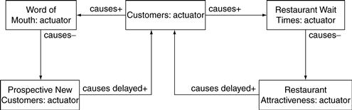
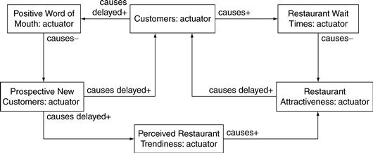
Rhonda builds such a business motivation simulation to explore how wait times affect the views of customers and potential customers. She starts with the causal loop diagram shown in Figure 11.22. As Zona becomes more popular and acquires more customers, word of mouth about the restaurant spreads. More prospective new customers try the restaurant. But as Zona becomes more popular, the customer wait time increases—both the time spent waiting for a table initially and the time spent waiting through the whole dining experience. As wait time increases, the attractiveness of Zona as a restaurant declines. And as Zona becomes less attractive, fewer customers go there; it becomes less popular.
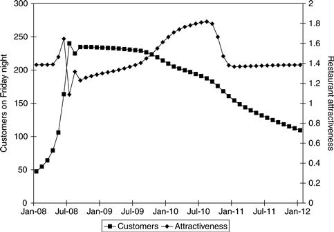
Rhonda sets the initial conditions of the model to reflect the number of customers Zona saw on Friday nights a year earlier. Similarly, she sets the wait times for those modest waits of a year earlier. Then she runs it for four simulated years, producing the results shown in Figure 11.23.
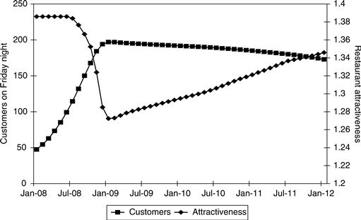
The simulation starts with 50 customers on a Friday night and with a very modest 30-minute average total wait time. Customers enjoy the good food and the modest waits. Word of mouth spreads. More people are attracted to Zona over the next 12 months, peaking at about 200 people on a Friday night. At that point there are 60-minute waits, and some customers find that those waits make Zona less attractive. Customers are gradually lost, and the wait times gradually decline.
Now Rhonda adds a complication. As more new customers discover Zona, some people start to perceive it as the hot new restaurant. This perception adds to Zona’s attractiveness, and more people dine there. The waits increase, but people care less about the long waits; eating at the latest place seems worth it. Of course, once the delays are long enough, people will be deterred from going to Zona, no matter how hot it is. The new causal loop diagram is shown in Figure 11.24.
The resulting simulation behaves differently. Figure 11.25 shows how customers and attractiveness play out over four years. Zona quickly becomes trendy, and Friday night customers approach 250, beyond the capacity of the restaurant. The waits increase to 90 minutes, but the trendiness offsets the impact of the long waits for a while, leading to high attractiveness. Of course, the perception of being the latest hot restaurant doesn’t last forever, and after a couple of years Zona loses some of the crowds and returns to being a very good restaurant with a loyal clientele.
But things are not quite so rosy. Rhonda now adds some more actuators to the causal loop diagram, as shown in Figure 11.26. She adds Former Customers, the number of people who were once customers of Zona but are customers no longer. Former customers also contribute to word of mouth, but their contribution is negative, not positive. The negative word of mouth serves to discourage people from trying Zona.
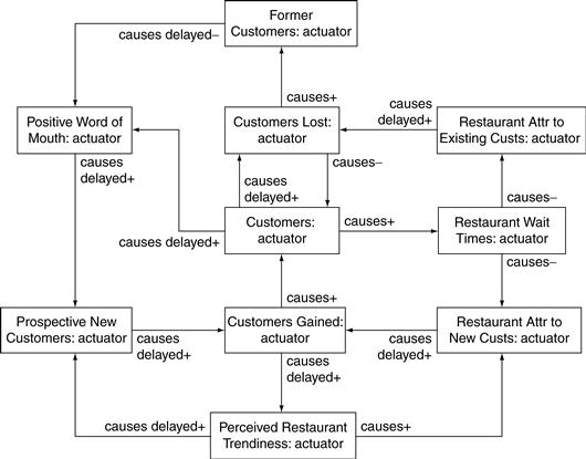
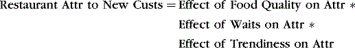
Rhonda separates restaurant attractiveness into two related measures of attractiveness. Restaurant Attr to New Custs is the degree to which Zona is attractive to new customers and includes the perceived trendiness. But once a customer is no longer new, he is less influenced by the trendiness. Now Restaurant Attr to Existing Custs is the relevant actuator. Rhonda also refines trendiness a bit, defining Perceived Restaurant Trendiness as caused by the number of new customers.
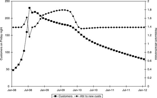
The results of the new model are shown in Figure 11.27. Again the waits spike early as Zona becomes trendy. But now the waits push existing customers away. When the trendiness passes, Zona continues to lose customers as the negative word of mouth from the former customers dominates the positive word of mouth. Zona never recovers.
Rhonda completes the model by adding a user interface so that restaurant managers can try different reservations policies and see the effects play out over time. (User interfaces are described later in this chapter, with Rhonda’s user interface shown as Figure 11.38.) If they want to let customers wait, they can see the sad results in Figure 11.27. They can also let their restaurant become a bit popular, then switch to the more restrictive policy of only seating people with reservations. Such a policy forgoes the revenues and some of the trendiness in return for keeping existing customers happier.
Business Motivation Simulation Tools
What does it take to simulate a motivation model? An appropriate simulation engine is required. Business process models are simulated with business process simulation engines, but business motivation models are simulated with a very different kind of engine—an engine suited for simulating strategy. A strategy simulation engine allows you to create a model of actuators influencing one another—like the one shown in Figure 11.26—and then simulate the results, producing a graph over time, like the one in Figure 11.27.
Variables
Creating a business motivation simulation requires more than just acquiring a modeling engine. Your motivation model must be ready for simulation. In particular, you must cast the model elements of your motivation model as variables, the key primitive of the motivation simulations.
What is a variable? A variable is some quantity that changes over time as the simulation is run. In the Zona simulation, Customers is a variable. The number of customers eating at Zona changes over the course of the simulation, first rising and then falling. Restaurant Wait Times is another variable.
Customers and Restaurant Wait Times are both concrete variables. A concrete variable is a variable that is measurable. You could in principle measure the value of either Customers or Restaurant Wait Times. You could keep track of the number of different people who eat at Zona at least once every three months to obtain a value for the Customers variable. Measuring Restaurant Wait Times is somewhat more involved, but with enough stopwatches you could time how long each party waits over the course of a single Friday night, then average those timings to obtain a value for Restaurant Wait Times.
Some variables are abstract, inherently difficult to measure. For example, it is not clear how you would measure Perceived Restaurant Trendiness. You could perhaps poll customers or prospective customers about what restaurant is hot, but your poll would not reflect the fact that some people’s opinions on these matters are more influential than others’.
Just because a variable is abstract does not mean it is less important. Some abstract variables are quite powerful; they have great influence on other variables. For example, perceptions of trendiness is a powerful motivator of behavior. Once a restaurant is perceived as the new hot place, many more people hear about it, and many more try it. A Zona model without a variable for trendiness will be less accurate and less valuable than one with trendiness.
Every variable—whether concrete or abstract—is measured in units against a scale. Customers is measured in the number of people who eat at Zona at least once over the course of three months. The scale of Customers is 0 to 50,000: 0 representing a restaurant empty all the time, and 50,000 far beyond the capacity of the rather small restaurant to serve.
Concrete variables have fairly obvious units and scales, but when you create a more abstract variable you often need to invent appropriate units and scale. For example, in the Zona simulation Perceived Restaurant Trendiness has a scale from 0 to 100. 0 is not trendy at all, and 100 is as trendy as it is possible to be, on everyone’s lips and in every newspaper article about top restaurants in DC.
Sometimes the appropriate unit of a variable is a rate over time. For example, in Figure 11.26 the actuator Customers Lost models how quickly Zona loses its existing customers—how quickly customers of Zona decide to stop patronizing that restaurant. The unit of Customers Lost is customers per week: how many customers does Zona lose each week? The scale for Customers Lost is 0 to 1,500. On a good week, Zona will lose no customers, and on a very bad week Zona might lose every customer who ventures in.
As you might have guessed, there is a relationship between the actuators in a causal loop diagram and variables in a motivation simulation. Every actuator is a variable. In Figure 11.26, there are 10 actuators, and each is a variable in the simulation; Former Customers, Restaurant Wait Times, and Positive Word of Mouth are all variables.
But there are more than 10 variables in the simulation model. In fact, Figure 11.26 is something of a simplification—accurate enough and shown to present a comprehensible view of the whole but without all the variables needed for simulation. For example, in Figure 11.26, Customers and Restaurant Wait Times are connected directly by a causes+ association. But to actually simulate that association, several more variables are needed. One such variable is Weekly Demand, as shown in Figure 11.28.
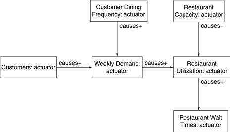
Defining Variables with Arithmetic
Sometimes the relationship between variables is expressed in simple arithmetic. For example, in Figure 11.28, the utilization of the restaurant is determined by dividing the weekly demand by the capacity:
![]()
The capacity is 1,300 customers (per week). When the weekly demand is 650, the utilization is 50 percent—on average, half the tables are occupied and half the tables are open.
The weekly demand is also expressed using simple arithmetic, by multiplying the number of customers by the frequency with which they dine:
![]()
Zona’s customers frequent the restaurant once every 12 weeks (on average), or at a frequency of 0.083/week. When Zona has 7,800 customers, the weekly demand is 650.
Defining Variables with Tables and Graphs
Often the relationship between variables is too complex to be modeled with simple arithmetic. For example, the relationship between the utilization of the restaurant and the average wait time for customers is not something easily defined by addition, multiplication, and the other primitives of arithmetic. Instead, we model it with a table of values, as shown in Table 11.2. When Zona is 20 percent utilized, the average wait time is 30 minutes. Customers wait only for their food to be prepared, not for a table, for waitstaff, or for their check. Higher levels of utilizations lead to longer waits. An average utilization of 60 percent for the week implies that Zona is quite busy at the busiest times—8:00 PM on Friday and Saturday nights. This leads to an average wait of 73 minutes. If the utilization is even higher, the waits are longer. A utilization of 90 percent leads to an average wait of 174 minutes, almost three hours.
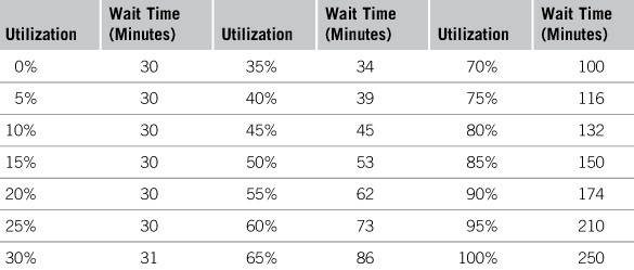
Of course, at any given time the utilization is likely to be some other value not shown in Table 11.2—not 55 or 60 percent, but 57.23 percent. The simulation engine finds the current value for wait time by interpolating—by creating an estimate of the value based on the two values on either side. The engine notes that 55 percent has a wait time of 62 minutes, that 60 percent has a wait time of 73 minutes, and that 57.23 percent has a wait time of 66.91 minutes, in between 62 and 73.
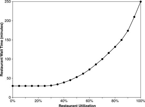
Some motivation simulation tools allow the modeler to define variable relationships graphically. The modeler has the choice of entering the values in Table 11.2 or drawing the equivalent graph shown in Figure 11.29.6 Often it is easier to think about the relationship in terms of a graph. Furthermore, most subject matter experts find the graph form easier to understand and validate.
Abstract Variables
Defining a relationship as a table or a graph is particularly useful for variables that are more abstract. For example, consider the attractiveness of Zona to customers. Attractiveness is very much an abstract variable, something we have modeled in the simulation on a 0 to 2 scale, with 2 being the most attractive restaurant in the world, 1.5 being quite attractive, 1 being neither particularly attractive nor particularly unattractive, and 0 being repellant to all customers. Attractiveness depends on the wait times as well as on other factors. But how does the average wait time influence the attractiveness of Zona? Clearly we are not going to create an arithmetic expression that shows how wait time influences attractiveness. But with tables and graphs, creating this relationship is surprisingly easy.
Consider first the causal loop diagram shown in Figure 11.30. The attractiveness of the restaurant to new customers is modeled by the variable Restaurant Attr to New Custs. In our model, restaurant attractiveness is determined not only by the wait times but also by the quality of the food and current trendiness of the restaurant. These three variables combine to determine attractiveness.
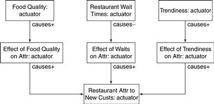
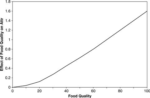
Each of the three variables could determine attractiveness on its own if the other two were not relevant. If the wait times at Zona were such that customers were not dissuaded, and if Zona were neither a currently trendy restaurant nor last year’s tired trend, then the attractiveness of Zona would be completely determined by the food quality: by how well the food delights the palates of the customers. The food quality is itself an abstract variable, with a range from 0 (awful) to 100 (world class). When the food quality is 0, the attractiveness will be 0, and when the food quality is 100, the attractiveness is 1.5, as shown in Figure 11.31.
Note that Figure 11.31 does not show the relationship between food quality and restaurant attractiveness directly. Rather it shows the relationship between food quality and the feeder variable Effect of Food Quality on Attr. That feeder variable is identical to restaurant attractiveness only if the other two factors have no effect on attractiveness. Mathematically that result is achieved by multiplying the effects for the three feeder variables:
If the waits are modest, the waiting time will have no effect on attractiveness. In this situation the feeder variable Effect of Waits on Attr will be 1.0. (And of course, multiplying by 1.0 leads to no change.) If the waits are long, the long waits will make Zona less attractive. In this case, Effect of Waits on Attr will be some number less than 1.0, and multiplying that number will reduce the attractiveness. Figure 11.32 shows the relationship between wait times and restaurant attractiveness.
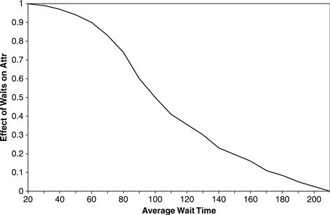
Long waits make Zona less attractive, dissuading would-be customers and convincing existing customers to eat elsewhere. For example, an average wait of 70 minutes—not uncommon at a busy restaurant—will lead to Effect of Waits on Attr taking a value of 0.83. When this is multiplied by the effect of the food quality and trendiness, the resulting attractiveness value will be 17 percent less than it would be otherwise, without the waits. But short waits in themselves never make Zona attractive. A fast-food restaurant might be attractive solely because it is fast, but a fine restaurant like Zona (and all the Mykonos restaurants) do not benefit from speed alone. Only food quality and trendiness can actually make Zona attractive in our model; Effect of Waits on Attr never takes a value greater than 1.
The third contributor to attractiveness—Trendiness—is also an abstract variable. Restaurant trendiness is measured on a 0 to 100 scale, with 0 being a restaurant that is yet to be discovered by the trend-setters and 100 a restaurant that is their favorite, at least today. Trendiness has its own effect on attractiveness and, like food quality, can contribute to Zona being either more attractive or less so.
Delays
Delays are common in business motivation situations. A corporate goal leads to new strategies, but forming the new strategies takes a while. An influencer occurs and is recognized as a threat, but only after someone within the organization notices it, brings it to the attention of others, and persuades enough people that the threat is real and something worth their consideration.
There are many delays in our restaurant wait simulation. For example, Zona’s reputation (modeled in Figure 11.26 as Positive Word of Mouth) leads to more prospective customers, people who want to eat at Zona. Some of these prospective customers will enjoy their experience and become Zona customers, eating there more or less regularly. But an increase in prospective customers does not lead to an immediate increase in customers, because the prospective customers do not drop all their other plans and immediately try Zona. Instead they work it into their schedules, they make reservations, they invite their friends or loved ones. It takes some time for a prospective customer to try Zona for the first time.
Figure 11.33 shows the relationship between Prospective New Customers and Customers Gained, expanded to include the intermediate variable Samplers not shown in the more abstract Figure 11.26. An increase in prospective new customers leads to an increase in samplers, people who try the restaurant. The increase happens after a delay as people fit the new restaurant in their plans. Once someone tries the restaurant for the first time, she is no longer a prospective new customer. So an increase in Samplers leads to a decrease in Prospective New Customers. Some of the people who sample the new restaurant then become customers, so there is a causes+ association from Samplers to Customers Gained.
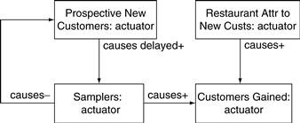
The causes delayed+ association from Prospective New Customers to Samplers is enough detail for the motivation model diagram of Figure 11.33 but not enough detail to actually drive a simulation. Simulation requires more precision. For example, Samplers could be defined as being exactly equal to Prospective New Customers but delayed by four weeks:
![]()
(As usual, we have employed precise English rather than bothering with the syntax of a delay function. In any case, the different simulation tools use different syntaxes for their delay functions, although they all offer this basic delay functionality.)
Figure 11.34 shows the simulation results for Samplers and Prospective New Customers. To better display the relationship, only a single 12-month period is shown, from July 2008 to July 2009. As you can see, Samplers follows the rise and fall of Prospective New Customers, after a four-week delay.
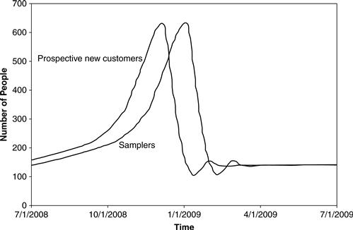
Pipeline Delay and Information Delay
In fact, several different kinds of delay are possible. The delay shown in Figure 11.34 is called a pipeline delay. In a pipeline delay the value of the lagging variable (Samplers) is exactly equal to the earlier value of the leading variable (Prospective New Customers). If there are 150 prospective customers on January 2, then four weeks later, on January 30, there will be 150 samplers trying the restaurant for the first time.
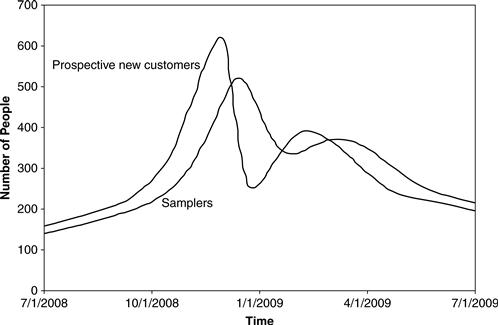
Pipeline delays are a good way to model situations where something needs a fixed amount of time to be prepared. If we were modeling the delay between the decision to offer a new menu and the actual introduction of the menu, a pipeline delay would be a good choice. But the delay between someone wanting to try Zona and that same person actually trying it for the first time is not a fixed delay. Some people plan ahead for 10 or 12 weeks, knowing when they will visit Washington, DC, and making reservations for that visit. Others plan a few weeks ahead, putting Zona on their social calendar. Still others are quite spontaneous, arranging to try Zona the day they hear about it. This diversity in planning behavior is better modeled by a different kind of delay, an information delay. With an information delay, some of the effect is almost immediate, some is delayed a bit, some delayed more, and some delayed even more.
The differing delay times can be averaged. For example, if some delay takes 1 day, some takes 2 weeks, and some takes 8 weeks, we might see an average delay of 4 weeks. So every information delay is expressed in terms of the average delay. For example, the relationship between Prospective New Customers and Samples might exhibit an information delay of 4 weeks:
![]()
Figure 11.35 shows the results of a four-week information delay. Note that the curve for samplers is smoother than the curve for prospective new customers. It does not reach as high during the peak of trendiness nor dip as low with the long waits. Information delays smooth out the extremes of the leading variable.
Simulating Feedback
In Chapter 3 we introduced causal loop diagrams, and earlier in this chapter we examined several of these diagrams. Within a causal loop diagram are typically one or more causal loops. A causal loop is a circular chain of variables affecting one another in turn. One variable affects a second variable, which in turn affects a third variable, and the third variable then affects the first. Or perhaps the loop is longer, with five or seven variables completing the circle.
Causal loops are common in the situations modeled by business motivation simulations. In the simulation of restaurant wait times we are exploring, there are at least 10 distinct causal loops. Using the terms introduced in Chapter 3 some of these loops are reinforcing; these loops drive more and more extreme behavior. For example, as the restaurant gains customers, more people talk about it. More prospective customers learn about the restaurant through word of mouth from their friends and colleagues. Some of these prospective customers try the restaurant, and some of those samplers like it so much that they become regular customers. This in turn leads to more word of mouth and further prospective customers. The restaurant becomes more and more popular.
Other loops in our restaurant example are balancing; these loops moderate the behavior, returning the situation to some middle ground. For example, as the restaurant earns new customers and it becomes more popular, the utilization grows and the wait times increase. The increasing wait times lead to a decline in the attractiveness and fewer new customers gained. Figure 11.36 shows this balancing causal loop.
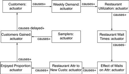
Of the nine variables in Figure 11.36, we have already explored six earlier in this chapter.
So we must define only the three remaining variables to completely model this causal loop, the three variables on the left of Figure 11.36: Enjoyed Proportion, Customers Gained, and Customers. Let’s start with Enjoyed Proportion. When new people sample Zona for the first time, how many enjoy their experience enough to become customers? How many do not enjoy their experience, at least not enough to return? The proportion of people who enjoy their experience is Enjoyed Proportion. For a world-class restaurant on a good day, the enjoyed proportion might be as high as 0.80; 80 percent of the new samplers like it. For a truly awful restaurant, the enjoyed proportion can be as low as 0.0—no one likes it enough to return.
Figure 11.37 shows how Enjoyed Proportion depends on Restaurant Attr to New Custs—the attractiveness of the restaurant to new customers. As you will recall, attractiveness varies from 0—not attractive at all—to 2—highly attractive.
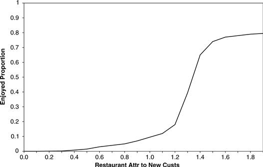
The second undefined variable—Customers Gained—is quite simple. It is just the number of people who sampled the restaurant this week multiplied by the proportion of those samplers that enjoyed their experience:
![]()
Stocks
Only one variable remains from Figure 11.36: Customers. The number of regular customers depends on how many regular customers were gained over the last week, on the variable Customers gained, as shown in Figure 11.36. Customers also depends on how many regular customers were lost in the last week, whether because they moved away, became bored with Zona, or suffered long waits during their latest Zona experience. (For simplicity Customers Lost is not shown in Figure 11.36.)
But Customers depends on something more than the customers lost and gained over the last week. A newly opened restaurant might gain 100 customers in its first week. In the same week, a long-established restaurant might also gain 100 customers. But they do not end the week with the same number of customers; the established restaurant already has hundreds of customers from its years of operation. The number of customers depends not only on how many customers are gained and lost that week but also on how many customers the restaurant had at the beginning of the week.
Customers is defined as the previous week’s value of Customers incremented by the newly arriving customers and decremented by the departing ones:
![]()
Most variables do not explicitly depend on their previous values. In our model, Enjoyed Proportion depends solely on the attractiveness of restaurants to new customers, not on any prior value of Enjoyed Proportion. Those variables (such as Customers) that are defined in terms of increments and decrements of prior values are called stocks.
Our restaurant wait model includes some other stocks. The number of former customers —the number of people who used to eat at Zona but no longer do—is modeled as a stock. Former Customers simply accumulates the values of Customers Lost:
![]()
Note that we do not draw the relationship between Customers and itself in a causal loop diagram. There is no association link from Customers back to itself in Figure 11.36.
Stocks are common in business motivation simulations. If we were to model Zona’s employees, we would model the skill of the chefs as a stock, with skill falling as new underchefs are hired and rising as chefs gain experience week after week. A model of the menu creation would include customer familiarity with the menu as a stock, rising week after week as the menu stayed the same and falling when changes were made. A model of the finances of Mykonos Corporation would include stocks for debts, capital equipment, and other balance sheet items. Anything that persists over time on its own accord is a candidate for being modeled as a stock.
User-Controlled Variables
In Chapter 2, we described playable simulations that a user can interact with as the simulation runs. A playable simulation does not merely show the user what would happen in a particular situation; a playable simulation turns over the steering wheel so that the user can try his hand at driving. Playable simulations are useful for teaching how to manage a situation and for the related task of persuading someone to take actions they would not otherwise consider.
A playable simulation has a user interface. The user interface allows the user to see what is happening as time progresses and to change some things. For example, Figure 11.38 shows a playable simulation of the restaurant wait model. In Figure 11.38, the user can see the wait times and the customer count and how those values have changed over the past few weeks.
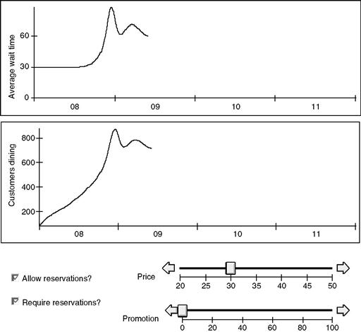
The user can also control things using the user interface in Figure 11.38. He can control whether reservations are taken and whether they are required. He might start 2008 by not taking any reservations, implement a reservations process midway through the year by checking the reservations taken box, and as Zona’s popularity increases, start requiring reservations. In other words, he can change things over the course of the simulation.
The user can control the price of dinner, raising prices as Zona gets more popular. And he can spend money on promotion. (For a high-end restaurant like Zona, promotion spending involves sponsoring high-profile charity events rather than coupons or radio advertisements that are typical for fast-food restaurants. But the effect is the same: greater awareness.)
There are two sliders in Figure 11.38, one for setting prices and the other for setting the promotion spending. Each slider controls a variable in the simulation. The price slider controls the variable Average Price, measured by the price of the average entrée. Unlike the other variables we have seen so far, Average Price is not affected by anything else in the simulation. Rather, it is completely controlled by the user and affects other simulation variables.
The two checkboxes in Figure 11.38 are also connected to variables. The lower checkbox is connected to the variable Require Reservations? which takes a value of true when reservations are required and false when they are not. Like Average Price, Require Reservations? is completely controlled by the user via the user interface. It affects other variables in the simulation model.
More About Simulating Business Motivation
We have just described an introduction to business motivation simulation, providing enough detail for you to build some simulations of strategies and other business motivation situations. When you are ready for more detail, there are many places to turn. Several books describe business motivation simulation. The best of these books (in our opinion) is John Sterman’s Business Dynamics: Systems Thinking and Modeling for a Complex World [Sterman 2000].
Of course, you need more than knowledge and skills to create a business motivation simulation. You also need a business simulation engine. Though many business modeling packages include a business process simulation engine, none includes a business motivation simulation engine, at least not at the time of this writing. You must acquire your business motivation simulation engine separately.
Validating a Simulation
As you will recall from Chapter 7, model verification involves improving the quality of a model by working with subject matter experts to check every model element in a model, and model validation is about improving the quality of a model through simulation. Now it is time to look at how model validation is performed and how simulation can be used to improve model quality.
Consider the business process of IT support: people handling support requests from employees, as shown in Figure 11.39. A phone call is answered by a level 1 technician. He understands the problem and perhaps resolves it on the phone. If he is not able to solve the problem himself, he may escalate it to a more experienced technician. Alternatively, the problem might be something that can only be solved in person, and the level 1 tech might dispatch a field tech to replace a part or reinstall key software.
The process shown in Figure 11.39 has been simulated for 10 (simulated) days, and some results of the simulation are shown above each activity. On the upper left of each activity are the activity job counts: how many tech support jobs are currently working that activity? For example, the activity Install Part or Software has an activity count of 6; six tech support problems are currently either being addressed by field techs replacing something, or are waiting for field techs to start working on their problems. On the upper right of each activity are the average activity times: For the jobs currently at the activity, how long have they been there, either being worked or waiting? The activity Install Part has an average activity time of 72 minutes; the six jobs there have been at that activity for (an average of) 72 minutes each.
Now consider what happens when a problem is escalated from the first level tech support to a more experienced second level. The level 2 tech starts by understanding the problem in the activity Understand Problem 2. This activity has an activity count of 419. There are 419 people on the phone, either talking to a level 2 tech or waiting for one to become available. Since there are only eight level 2 techs in total, most customers must be waiting. The activity time is 40 hours—the 419 people have waited an average of 40 hours on the phone at this task.
Figure 11.40 shows a graph of the activity job count for Understand Problem 2 over the 10 simulated days. The count has accumulated, growing day by day until it has reached 419 jobs on day 10. Clearly something in the model is causing a growing backlog of people waiting at this activity.
This activity job count does not reflect reality. No one has waited 40 hours on the phone for a level 2 tech. Something is wrong with the model and needs to be corrected.7 There are several model problems that could cause this growing backlog in the simulation. Perhaps too many jobs are being sent to level 2 techs because the decision logic in the gateway Problem Resolved? is faulty. Perhaps too much time is being spent by level 2 techs; they actually finish their work in less time than the simulation indicates and so the backlog does not accumulate. Perhaps there are more level 2 techs in reality than in the simulation. It is even possible that some backlogs do accumulate for level 2 tech support, and after 10 or 20 minutes, the people on the phone give up, hang up, and try to fix the problem themselves.
Whatever the reason for the backlog, the model needs to be corrected to reflect the reality that is occurring. You need to question your subject matter experts to determine what needs to be fixed so that the simulation results provide useful data for your questions. You do not need to ask about the 40-hour backlog—you already know it is not valid. But you can ask questions to investigate sources of this backlog. You can ask whether the simulated activity time spent on Understand Problem 2 is accurate. You can check the percentage utilization of tech 2s in the simulation and compare that to the subject matter expert’s understanding. This process is model validation: using the simulation results to drill into the model until you discover the root cause of the problem.
An ever-increasing backlog is one simulation result that is useful for validating a business process model. There are three others that are often used:
![]() Resource utilization; for example, a resource is 40% utilized in the simulation, but much busier in the real world
Resource utilization; for example, a resource is 40% utilized in the simulation, but much busier in the real world
![]() Job cycle time; for example, some jobs take two weeks to process in the end-to-end simulation, but in the real world everything is done within four days
Job cycle time; for example, some jobs take two weeks to process in the end-to-end simulation, but in the real world everything is done within four days
![]() Job touch time; for example, some jobs are only worked by resources for 20 minutes, but in the real world every job is worked for at least an hour
Job touch time; for example, some jobs are only worked by resources for 20 minutes, but in the real world every job is worked for at least an hour
Business motivation models can also be validated. As with business process validation, you compare simulated results with real-world values. But instead of comparing activity job counts or cycle times, you compare the results produced by motivation simulations: market shares, customers, morale, and so on.
Simulation and Standards
The current version of BPMN at the time of this writing—BPMN 1.1—does not support business process simulation. Many activity attributes described in this chapter and needed for simulation are not part of BPMN: there is no duration attribute, no resourceShift attribute, no intrinsicDelay, and no consistentResource. BPMN does not specify modeling support for resources beyond the participant that labels a swimlane, and does not specify modeling support for jobs beyond the ability to set job attributes from an activity.
As discussed earlier in this chapter, start events create simulation jobs according to schedules and quantities specified in the start event itself. The BPMN spec does not include these attributes: there is no jobQuantity, jobInterval, or jobStartDuration. Many tools do support process simulation, in non-standardized ways.
As you may recall from Chapter 5, some start events are timers. A timer models the special case of work starting because it is the right day or time to start. For example, Mykonos central accounting reconciles electronic credit card receipts from the restaurants with the payments from the merchant banks. This process occurs every weekday morning, and the model begins work with a start event, 8:00 AM every weekday.
There is a subtle and important distinction between the timer start events (as described in BPMN) and the simulation of start events as described in this chapter. In BPMN, only some start events are properly modeled as timers. It does not make sense to model the arrival of diners with a timer. They arrive not because they eat at Zona at a certain day and time but instead for their own reasons: some are there for business meetings, others on dates, still others to meet with friends. We use jobQuantity and the rest of the simulation-specific attributes as a model approximation of their own logic, not because the process is inherently started by a time occurrence.
BPMN specifies some support for jobs—calling them “tokens” in the specification. An activity (or event or gateway) can assign a value to a modeler-defined attribute of a job as the job passes through the activity (or event or gateway). This support for job attribute assignment is intended primarily for executing a process in a process engine (as described in Chapter 12), but job attribute assignment can also be used for simulating the same process in a simulation engine.
Business Process Simulation Tooling
The good news is that some BPMN-compliant modeling tools do support business process simulation. Of course all these tools support it all differently. The tools available today support simulation to different degrees. For example, we have worked with a commercial tool that supports activities and resources but not jobs. Within this tool there is no way to make a gateway branch depend on the characteristic of the jobs that pass through it, as described earlier in this chapter.
Existing tools also support the same capability in different ways. Every tool that simulates supports capturing the duration of an activity, but there are wide differences in how that duration is modeled.
Standard Support for Business Motivation Simulation
There are a few tools that support business motivation simulation. Each tool is different, with a different modeling language and somewhat different capabilities. As of today, there are no standards for simulating business motivation.
To simulate a business process model, you must first prepare it for simulation. You must provide durations and delays for the activities. You must indicate how jobs are divided at gateways. You must create schedules for jobs that are to be created at start events. And you must model resources, their availability, and their costs.
Once a business process model is prepared, a simulation engine can simulate it, giving you costs, cycle times, touch times, and other statistical results that are difficult to determine with any kind of other static analysis.
Preparation is also required to simulate a business motivation model. The preparation involves defining variables. Most of these variables are dependent on other variables. Some are defined via arithmetic expressions. Some are defined via tables and graphs. Some variables are stocks, and defined by how other variables cause them to change from the values they already have. And some variables are defined by users in real-time, taking a value when a user changes a user interface control.
Once prepared, a motivation model is simulated by a business motivation engine. The result shows market share over time, customers gained or lost, morale changes, or whatever is the topic of the business motivation model.
Chapter 12 describes how to execute a model, and turn it into a software application that a business can use.
1As with Figure 10.8, Figure 11.8 is the simpler customer dining process originally introduced in Chapter 2, not the more complex process—with subprocesses—from Chapter 5.
2In much of the BPMN literature, jobs are called tokens. This reflects BPMN’s theoretical basis in Petri nets. For modeling, we prefer the term job instead of token because it is a more natural description of a party of restaurant customers, an insurance claim, or whatever is flowing through the process.
3For a large party, there is a greater chance that someone in the party will order a dinner that takes a long time to prepare. In a higher-fidelity model, the duration of Cook Dinner could be made dependent on the size of the party, albeit still random.
4Most business process models include this kind of random behavior in gateway branching, activity durations, or resource allocations. To get reliable results, you need to run a simulation long enough to overcome temporary effects. Alternatively, you can run a short simulation multiple times.
5As usual, modeling tools vary in the syntax of values for these start event attributes. In this book, we use a structured English for readability.
6Note that the graph shown in Figure 11.29 is fundamentally different from earlier graphs in this chapter. Earlier graphs showed the results of simulations. Figure 11.29 defines a variable in the simulation model itself, a variable used to produce simulation results.
7Or possibly nothing is wrong with the model and this one run of the simulation is just unusual. Most simulation models rely on randomness to some degree. An activity takes between 1 and 10 minutes, and the actual time for any given job is a random quantity between 1 and 10. A gateway sends 40 percent of the jobs up and 60 percent down, and whether a particular job goes up or down depends on a random chance. Usually business process simulations are not very sensitive to the randomness. If you run the same simulation again, you will get different results, but similar to the first time. And if you run it a third time, the results will be similar to the first and second runs.
But some simulation models are very sensitive to the random quantities used [Law 2006]. And even for a model that is not so sensitive, it is possible—though unlikely—to have a run with radically different results. Reliability analysis of the results of a simulation is important but beyond the scope of this book.