
Chapter 11
Application Case Study
Advanced MRI Reconstruction
Chapter Outline
11.1 Application Background
11.2 Iterative Reconstruction
11.3 Computing FHD
11.4 Final Evaluation
11.5 Exercises
Application case studies teach computational thinking and practical programming techniques in a concrete manner. They also help demonstrate how the individual techniques fit into a top-to-bottom development process. Most importantly, they help us to visualize the practical use of these techniques in solving problems. In this chapter, we start with the background and problem formulation of a relatively simple application. We show that parallel execution not only speeds up the existing approaches, but also allows applications experts to pursue approaches that are known to provide benefit but were previously ignored due to their excessive computational requirements. We then use an example algorithm and its implementation source code from such an approach to illustrate how a developer can systematically determine the kernel parallelism structure, assign variables into CUDA memories, steer around limitations of the hardware, validate results, and assess the impact of performance improvements.
11.1 Application Background
Magnetic resonance imaging (MRI) is commonly used by the medical community to safely and noninvasively probe the structure and function of biological tissues in all regions of the body. Images that are generated using MRI have made profound impact in both clinical and research settings. MRI consists of two phases: acquisition (scan) and reconstruction. During the acquisition phase, the scanner samples data in the k-space domain (i.e., the spatial-frequency domain or Fourier transform domain) along a predefined trajectory. These samples are then transformed into the desired image during the reconstruction phase.
The application of MRI is often limited by high noise levels, significant imaging artifacts, and/or long data acquisition times. In clinical settings, short scan times not only increase scanner throughput but also reduce patient discomfort, which tends to mitigate motion-related artifacts. High image resolution and fidelity are important because they enable earlier detection of pathology, leading to improved prognoses for patients. However, the goals of short scan time, high resolution, and high signal-to-noise ratio (SNR) often conflict; improvements in one metric tend to come at the expense of one or both of the others. One needs new technological breakthroughs to be able to simultaneously improve on all of three dimensions. This study presents a case where massively parallel computing provides such a breakthrough.
Readers are referred to MRI textbooks such as Liang and Lauterbur [LL1999] for the physics principles behind MRI. For this case study, we will focus on the computational complexity in the reconstruction phase and how the complexity is affected by the k-space sampling trajectory. The k-space sampling trajectory used by the MRI scanner can significantly affect the quality of the reconstructed image, the time complexity of the reconstruction algorithm, and the time required for the scanner to acquire the samples. Equation (11.1) below shows a formulation that relates the k-space samples to the reconstructed image for a class of reconstruction methods.
![]() (11.1)
(11.1)
In Eq. (11.1), m(r) is the reconstructed image, s(k) is the measured k-space data, and W(k) is the weighting function that accounts for nonuniform sampling. That is, W(k) decreases the influence of data from k-space regions where a higher density of sample points are taken. For this class of reconstructions, W(k) can also serve as an apodization function that reduces the influence of noise and reduces artifacts due to finite sampling.
If data is acquired at uniformly spaced Cartesian grid points in the k-space under ideal conditions, then the W(k) weighting function is a constant and can thus be factored out of the summation in Eq. (11.1). As a result, the reconstruction of m(r) becomes an inverse fast Fourier transform (FFT) on s(k), an extremely efficient computation method. A collection of data measured at such uniformed spaced Cartesian grid points is referred to as a Cartesian scan trajectory, depicted in Figure 11.1(a). In practice, Cartesian scan trajectories allow straightforward implementation on scanners and are widely used in clinical settings today.
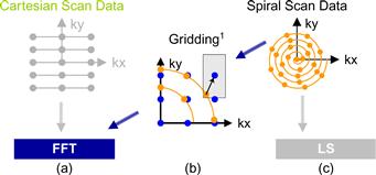
Figure 11.1 Scanner k-space trajectories and their associated reconstruction strategies: (a) Cartesian trajectory with FFT reconstruction, (b) spiral (or non-Cartesian trajectory in general) followed by gridding to enable FFT reconstruction, and (c) spiral (non-Cartesian) trajectory with linear solver–based reconstruction.
Although the inverse FFT reconstruction of Cartesian scan data is computationally efficient, non-Cartesian scan trajectories often have advantages in reduced sensitivity to patient motion, better ability to provide self-calibrating field inhomogeneity information, and reduced requirements on scanner hardware performance. As a result, non-Cartesian scan trajectories like spirals (shown in Figure 11.1c), radial lines (projection imaging), and rosettes have been proposed to reduce motion-related artifacts and address scanner hardware performance limitations. These improvements have recently allowed the reconstructed image pixel values to be used for measuring subtle phenomenon such as tissue chemical anomalies before they become anatomical pathology. Figure 11.2 shows such a measurement that generates a map of sodium, a heavily regulated substance in normal human tissues. The information can be used to track tissue health in stroke and cancer treatment processes. The variation or shifting of sodium concentration gives early signs of disease development or tissue death. For example, the sodium map of a human brain shown in Figure 11.2 can be used to give an early indication of brain tumor tissue responsiveness to chemotherapy protocols, enabling individualized medicine. Because sodium is much less abundant than water molecules in human tissues, a reliable measure of sodium levels requires a higher SNR through a higher number of samples and needs to control the extra scan time with non-Cartesian scan trajectories.
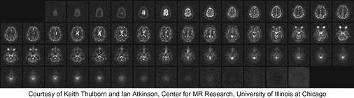
Figure 11.2 The use of non-Cartesian k-space sample trajectory and accurate linear solver–based reconstruction enables new MRI modalities with exciting medial applications. The improved SNR enables reliable collection of in-vivo concentration data on a chemical substance such as sodium in human tissues. The variation or shifting of sodium concentration gives early signs of disease development or tissue death. For example, the sodium map of a human brain shown in this Figure can be used to give early indication of brain tumor tissue responsiveness to chemo-therapy protocols, enabling individualized medicine.
Image reconstruction from non-Cartesian trajectory data presents both challenges and opportunities. The main challenge arises from the fact that the exponential terms are no longer uniformly spaced; the summation does not have the form of an FFT anymore. Therefore, one can no longer perform reconstruction by directly applying an inverse FFT to the k-space samples. In a commonly used approach called gridding, the samples are first interpolated onto a uniform Cartesian grid and then reconstructed using the FFT (see Figure 11.1b). For example, a convolution approach to gridding takes a k-space data point, convolves it with a gridding kernel, and accumulates the results on a Cartesian grid. Convolution is quite computationally intensive. Accelerating gridding computation on many-core processors facilitates the application of the current FFT approach to non-Cartesian trajectory data. Since we have already studied the convolution pattern in Chapter 8 and will be examining a convolution-style computation in Chapter 12, we will not cover it here.
In this chapter, we will cover an iterative, statistically optimal image reconstruction method that can accurately model imaging physics and bound the noise error in each image pixel value. However, such iterative reconstructions have been impractical for large-scale 3D problems due to their excessive computational requirements compared to gridding. Recently, these reconstructions have become viable in clinical settings when accelerated on GPUs. In particular, we will show that an iterative reconstruction algorithm that used to take hours using a high-end sequential CPU now takes only minutes using both CPUs and GPUs for an image of moderate resolution, a delay acceptable in clinical settings.
11.2 Iterative Reconstruction
Haldar, et al [HHB 2007] proposed a linear solver–based iterative reconstruction algorithm for non-Cartesian scan data, as shown in Figure 11.1(c). The algorithm allows for explicit modeling and compensation for the physics of the scanner data acquisition process, and can thus reduce the artifacts in the reconstructed image. It is, however, computationally expensive. The reconstruction time on high-end sequential CPUs has been hours for moderate-resolution images and thus impractical in clinical use. We use this as an example of innovative methods that have required too much computation time to be considered practical. We will show that massive parallelism can reduce the reconstruction time to the order of a minute so that one can deploy the new MRI modalities such as sodium imaging in clinical settings.
Figure 11.3 shows a solution of the quasi-Bayesian estimation problem formulation of the iterative linear solver–based reconstruction approach, where ρ is a vector containing voxel values for the reconstructed image, F is a matrix that models the physics of imaging process, D is a vector of data samples from the scanner, and W is a matrix that can incorporate prior information such as anatomical constraints. In clinical settings, the anatomical constraints represented in W are derived from one or more high-resolution, high-SNR water molecule scans of the patient. These water molecule scans reveal features such as the location of anatomical structures. The matrix W is derived from these reference images. The problem is to solve for ρ given all the other matrices and vectors.
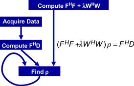
Figure 11.3 An iterative linear solver–based approach to reconstruction of no-Cartesian k-space sample data.
On the surface, the computational solution to the problem formulation in Figure 11.3 should be very straightforward. It involves matrix–matrix multiplications and addition (FHF+λWHW), matrix–vector multiplication (FHD), matrix inversion (FHF+λWHW)−1, and finally matrix–matrix multiplication ((FHF+λWHW)−1×FHD). However, the sizes of the matrices make this straightforward approach extremely time consuming. FH and F are 3D matrices of which the dimensions are determined by the resolution of the reconstructed image ρ. Even in a modest resolution 1283-voxel reconstruction, there are 1283 columns in F with N elements in each column where N is the number of k-space samples used. Obviously, F is extremely large.
The sizes of the matrices involved are so large that the matrix operations involved in a direct solution of the equation in Figure 11.3 are practically intractable. An iterative method for matrix inversion, such as the conjugate gradient (CG) algorithm, is therefore preferred. The conjugate gradient algorithm reconstructs the image by iteratively solving the equation in Figure 11.3 for ρ. During each iteration, the CG algorithm updates the current image estimate ρ to improve the value of the quasi-Bayesian cost function. The computational efficiency of the CG technique is largely determined by the efficiency of matrix–vector multiplication operations involving FHF+λWHW and ρ, as these operations are required during each iteration of the CG algorithm.
Fortunately, matrix W often has a sparse structure that permits efficient multiplication by WHW, and matrix FHF is Toeplitz that enables efficient matrix–vector multiplication via the FFT. Stone et al. [SHT2008] present a GPU-accelerated method for calculating Q, a data structure that allows us to quickly calculate matrix–vector multiplication involving FHF without actually calculating FHF itself. The calculation of Q can take days on a high-end CPU core. It only needs to be done once for a given trajectory and can be used for multiple scans.
The matrix–vector multiply to calculate FHD takes about one order of magnitude less time than Q but can still take about three hours for a 1283-voxel reconstruction on a high-end sequential CPU. Since FHD needs to be computed for every image acquisition, it is desirable to reduce the computation time of FHD to minutes.1 We will show the details of this process. As it turns out, the core computational structure of Q is identical to that of FHD. As a result, the same methodology can be used to accelerate the computation of both.
The “find ρ” step in Figure 11.3 performs the actual CG based on FHD. As we explained earlier, precalculation of Q makes this step much less computationally intensive than FHD, and accounts for only less than 1% of the execution of the reconstruction of each image on a sequential CPU. As a result, we will leave it out of the parallelization scope and focus on FHD in this chapter. We will, however, revisit its status at the end of the chapter.
11.3 Computing FHD
Figure 11.4 shows a sequential C implementation of the computations for the core step of computing a data structure for multiplications with FHF (referred to as Q computation in Figure 11.4a) without explicitly calculating FHF, and that for FHD (Figure 11.4b). It should be clear from a quick glance at Figures 11.4(a) and (b) that the core steps of Q and FHD have identical structures. Both computations start with an outer loop that encloses an inner loop. The only differences are the particular calculation done in each loop body and the fact that the core step of Q involves a much larger m, since it implements a matrix–matrix multiplication as opposed to a matrix–vector multiplication, thus it incurs a much longer execution time. Thus, it suffices to discuss one of them. We will focus on FHD, since this is the one that will need to be run for each image being reconstructed.
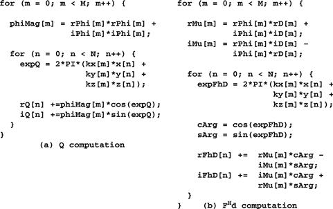
Figure 11.4 Computation of (a) Q and (b) FHD.
A quick glance at Figure 11.4(b) shows that the C implementation of FHD is an excellent candidate for acceleration on the GPU because it exhibits substantial data parallelism. The algorithm first computes the real and imaginary components of Mu (rMu and iMu) at each sample point in the k-space. It then computes the real and imaginary components of FHD at each voxel in the image space. The value of FHD at any voxel depends on the values of all k-space sample points. However, no voxel elements of FHD depend on any other elements of FHD. Therefore, all elements of FHD can be computed in parallel. Specifically, all iterations of the outer loop can be done in parallel and all iterations of the inner loop can be done in parallel. The calculations of the inner loop, however, have a dependence on the calculation done by the preceding statements in the same iteration of the outer loop.
Despite the algorithm’s abundant inherent parallelism, potential performance bottlenecks are evident. First, in the loop that computes the elements of FHD, the ratio of floating-point operations to memory accesses is at best 3:1 and at worst 1:1. The best case assumes that the sin and cos trigonometry operations are computed using the five-element Taylor series that requires 13 and 12 floating-point operations, respectively. The worst case assumes that each trigonometric operation is computed as a single operation in hardware. As we have seen in Chapter 5, a floating-point to memory access ratio of 16:1 or more is needed for the kernel to not be limited by memory bandwidth. Thus, the memory accesses will clearly limit the performance of the kernel unless the ratio is drastically increased.
Second, the ratio of floating-point arithmetic to floating-point trigonometry functions is only 13:2. Thus, a GPU-based implementation must tolerate or avoid stalls due to long-latency sin and cos operations. Without a good way to reduce the cost of trigonometry functions, the performance will likely be dominated by the time spent in these functions.
We are now ready to take the steps in converting FHD from sequential C code to a CUDA kernel.
Step 1: Determine the Kernel Parallelism Structure
The conversion of a loop into a CUDA kernel is conceptually straightforward. Since all iterations of the outer loop of Figure 11.4(b) can be executed in parallel, we can simply convert the outer loop into a CUDA kernel by mapping its iterations to CUDA threads. Figure 11.5 shows a kernel from such a straightforward conversion. Each thread implements an iteration of the original outer loop. That is, we use each thread to calculate the contribution of one k-space sample to all FHD elements. The original outer loop has M iterations, and M can be in the millions. We obviously need to have multiple thread blocks to generate enough threads to implement all these iterations.
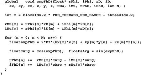
Figure 11.5 First version of the FHD kernel. The kernel will not execute correctly due to conflicts between threads in writing into rFhD and iFhD arrays.
To make performance tuning easy, we declare a constant FHD_THREADS_PER_BLOCK that defines the number of threads in each thread block when we invoke the cmpFHd kernel. Thus, we will use M/FHD_THREADS_PER_BLOCK for the grid size (in terms of number of blocks) and FHD_THREADS_PER_BLOCK for block size (in terms of number of threads) for kernel invocation. Within the kernel, each thread calculates the original iteration of the outer loop that it is assigned to cover using the formula blockIdx.x ∗ FHD_THREADS_PER_BLOCK + threadIdx.x. For example, assume that there are 65,536 k-space samples and we decided to use 512 threads per block. The grid size at kernel innovation would be 65,536÷512=128 blocks. The block size would be 512. The calculation of m for each thread would be equivalent to blockIdx.x∗512 + threadIdx.
While the kernel of Figure 11.5 exploits ample parallelism, it suffers from a major problem: all threads write into all rFhD and iFhD voxel elements. This means that the kernel must use atomic operations in the global memory in the inner loop to keep threads from trashing each other’s contributions to the voxel value. This can seriously affect the performance of the kernel. Note that as is, the code will not even execute correctly since no atomic operation is used. We need to explore other options.
The other option is to use each thread to calculate one FhD value from all k-space samples. To do so, we need to first swap the inner loop and the outer loop so that each of the new outer loop iterations processes one FhD element. That is, each of the new outer loop iterations will execute the new inner loop that accumulates the contribution of all k-space samples to the FhD element handled by the outer loop iteration. This transformation to the loop structure is called loop interchange. It requires a perfectly nested loop, meaning that there is no statement between the outer for loop statement and the inner for loop statement. This is, however, not true for the FHD code in Figure 11.4(b). We need to find a way to move the calculation of rMu and iMu elements out of the way.
From a quick inspection of Figure 11.6(a), which is a replicate of Figure 11.4(b), we see that the FHD calculation can be split into two separate loops, as shown in Figure 11.6(b), using a technique called loop fission or loop splitting. This transformation takes the body of a loop and splits it into two loops. In the case of FHD, the outer loop consists of two parts: the statements before the inner loop and the inner loop. As shown in Figure 11.6(b), we can perform loop fission on the outer loop by placing the statements before the inner loop into a loop and the inner loop into a second loop. The transformation changes the relative execution order of the two parts of the original outer loop. In the original outer loop, both parts of the first iteration execute before the second iteration. After fission, the first part of all iterations will execute; they are then followed by the second part of all iterations. Readers should be able to verify that this change of execution order does not affect the execution results for FHD. This is because the execution of the first part of each iteration does not depend on the result of the second part of any preceding iterations of the original outer loop. Loop fission is a transformation often done by advanced compilers that are capable of analyzing the (lack of) dependence between statements across loop iterations.
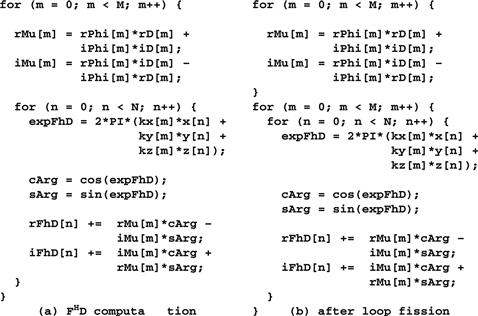
Figure 11.6 (a) Loop fission on the FHD computation and (b) after loop fission.
With loop fission, the FHD computation is now done in two steps. The first step is a single-level loop that calculates the rMu and iMu elements for use in the second loop. The second step corresponds to the loop that calculates the FhD elements based on the rMu and iMu elements calculated in the first step. Each step can now be converted into a CUDA kernel. The two CUDA kernels will execute sequentially with respect to each other. Since the second loop needs to use the results from the first loop, separating these two loops into two kernels that execute in sequence does not sacrifice any parallelism.
The cmpMu() kernel in Figure 11.7 implements the first loop. The conversion of the first loop from sequential C code to a CUDA kernel is straightforward: each thread implements one iteration of the original C code. Since the M value can be very big, reflecting the large number of k-space samples, such a mapping can result in a large number of threads. With 512 threads in each block, we will need to use multiple blocks to allow the large number of threads. This can be accomplished by having a number of threads in each block, specified by MU_THREADS_PER_BLOCK in Figure 11.4(c), and by employing M/MU_THREADS_PER_BLOCK blocks needed to cover all M iterations of the original loop. For example, if there are 65,536 k-space samples, the kernel could be invoked with a configuration of 512 threads per block and 65,536÷512=128 blocks. This is done by assigning 512 to MU_THREADS_PER_BLOCK and using MU_THREADS_PER_BLOCK as the block size and M/MU_THREADS_PER_BLOCK as the grid size during kernel innovation.
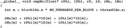
Figure 11.7 cmpMu kernel.
Within the kernel, each thread can identify the iteration assigned to it using its blockIdx and threadIdx values. Since the threading structure is one dimensional, only blockIdx.x and threadIdx.x need to be used. Because each block covers a section of the original iterations, the iteration covered by a thread is blockIdx.x∗MU_THREADS_PER_BLOCK + threadIdx. For example, assume that MU_THREADS_PER_BLOCK=512. The thread with blockIdx.x=0 and threadIdx.x=37 covers the 37th iteration of the original loop, whereas the thread with blockIdx.x=5 and threadIdx.x=2 covers the 2,562nd (5×512+2) iteration of the original loop. Using this iteration number to access the Mu, Phi, and D arrays ensures that the arrays are covered by the threads in the same way they were covered by the iterations of the original loop. Because every thread writes into its own Mu element, there is no potential conflict between any of these threads.
Determining the structure of the second kernel requires a little more work. An inspection of the second loop in Figure 11.6(b) shows that there are at least three options in designing the second kernel. In the first option, each thread corresponds to one iteration of the inner loop. This option creates the most number of threads and thus exploits the largest amount of parallelism. However, the number of threads would be N×M, with both N in the range of millions and M in the range of hundreds of thousands. Their product would result in too many threads in the grid.
A second option is to use each thread to implement an iteration of the outer loop. This option employs fewer threads than the first option. Instead of generating N×M threads, this option generates M threads. Since M corresponds to the number of k-space samples and a large number of samples (on the order of a hundred thousand) are typically used to calculate FHD, this option still exploits a large amount of parallelism. However, this kernel suffers the same problem as the kernel in Figure 11.5. That is, each thread will write into all rFhD and iFhD elements, thus creating an extremely large number of conflicts between threads. As is the case of Figure 11.5, the code in Figure 11.8 will not execute correctly without adding atomic operations that will significantly slow down the execution. Thus, this option does not work well.

Figure 11.8 Second option of the FHD kernel.
A third option is to use each thread to compute one pair of rFhD and iFhD elements. This option requires us to interchange the inner and outer loops and then use each thread to implement an iteration of the new outer loop. The transformation is shown in Figure 11.9. Loop interchange is necessary because the loop being implemented by the CUDA threads must be the outer loop. Loop interchange makes each of the new outer loop iterations process a pair of rFhD and iFhD elements. Loop interchange is permissible here because all iterations of both levels of loops are independent of each other. They can be executed in any order relative to one another. Loop interchange, which changes the order of the iterations, is allowed when these iterations can be executed in any order. This option generates N threads. Since N corresponds to the number of voxels in the reconstructed image, the N value can be very large for higher-resolution images. For a 1283 images, there are 1283=2,097,152 threads, resulting in a large amount of parallelism. For higher resolutions, such as 5123, we may need to invoke multiple kernels, and each kernel generates the value of a subset of the voxels. Note these threads now all accumulate into their own rFhD and iFhd elements since every thread has a unique n value. There is no conflict between threads. These threads can run totally in parallel. This makes the third option the best choice among the three options.
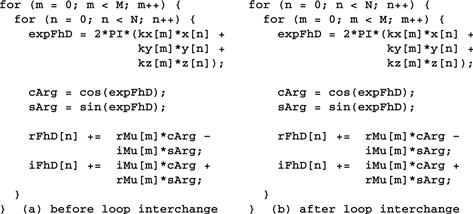
Figure 11.9 Loop interchange of the FHD computation.
The kernel derived from the interchanged loops is shown in Figure 11.10. The threads are organized as a two-level structure. The outer loop has been stripped away; each thread covers an iteration of the outer (n) loop, where n is equal to blockIdx.x∗FHD_THREADS_PER_BLOCK + threadIdx.x. Once this iteration (n) value is identified, the thread executes the inner loop based on that n value. This kernel can be invoked with a number of threads in each block, specified by a global constant FHD_THREADS_PER_BLOCK. Assuming that N is the variable that gives the number of voxels in the reconstructed image, N/FHD_THREADS_PER_BLOCK blocks cover all N iterations of the original loop. For example, if there are 65,536 k-space samples, the kernel could be invoked with a configuration of 512 threads per block and 65,536÷512=128 blocks. This is done by assigning 512 to FHD_THREADS_PER_BLOCK and using FHD_THREADS_PER_BLOCK as the block size and N/FHD_THREADS_PER_BLOCK as the grid size during kernel innovation.
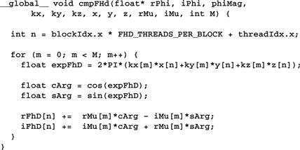
Figure 11.10 Third option of the FHD kernel.
Step 2: Getting Around the Memory Bandwidth Limitation
The simple cmpFhD kernel in Figure 11.10 will provide limited speedup due to memory bandwidth limitations. A quick analysis shows that the execution is limited by the low compute to memory access ratio of each thread. In the original loop, each iteration performs at least 14 memory accesses: kx[m], ky[m], kz[m], x[n], y[n], z[n], rMu[m] twice, iMu[m] twice, rFhD[n] read and write, and iFhD[n] read and write. Meanwhile, about 13 floating-point multiply, add, or trigonometry operations are performed in each iteration. Therefore, the compute to memory access ratio is approximately 1, which is too low according to our analysis in Chapter 5.
We can immediately improve the compute to memory access ratio by assigning some of the array elements to automatic variables. As we discussed in Chapter 5, the automatic variables will reside in registers, thus converting reads and writes to the global memory into reads and writes to on-chip registers. A quick review of the kernel in Figure 11.10 shows that for each thread, the same x[n], y[n], and z[n] elements are used across all iterations of the for loop. This means that we can load these elements into automatic variables before the execution enters the loop.2 The kernel can then use the automatic variables inside the loop, thus converting global memory accesses to register accesses. Furthermore, the loop repeatedly reads from and writes into rFhD[n] and iFhD[n]. We can have the iterations read from and write into two automatic variables and only write the contents of these automatic variables into rFhD[n] and iFhD[n] after the execution exits the loop. The resulting code is shown in Figure 11.11. By increasing the number of registers used by 5 for each thread, we have reduced the memory access done in each iteration from 14 to 7. Thus, we have increased the compute to memory access ratio from 13:14 to 13:7. This is a very good improvement and a good use of the precious register resource.
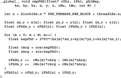
Figure 11.11 Using registers to reduce memory accesses in the FHD kernel.
Recall that the register usage can limit the number of blocks that can run in a streaming multiprocessor (SM). By increasing the register usage by 5 in the kernel code, we increase the register usage of each thread block by 5∗FHD_THREADS_PER_BLOCK. Assuming that we have 128 threads per block, we just increased the block register usage by 640. Since each SM can accommodate a combined register usage of 65,536 registers among all blocks assigned to it (at least in SM version 3.5), we need to be careful, as any further increase of register usage can begin to limit the number of blocks that can be assigned to an SM. Fortunately, the register usage is not a limiting factor to parallelism for this kernel.
We want to further improve the compute to memory access ratio to something closer to 10:1 by eliminating more global memory accesses in the cmpFHD kernel. The next candidates to consider are the k-space samples kx[m], ky[m], and kz[m]. These array elements are accessed differently than the x[n], y[n], and z[n] elements: different elements of kx, ky, and kz are accessed in each iteration of the loop in Figure 11.11. This means that we cannot load each k-space element into an automatic variable register and access that automatic variable off a register through all the iterations. So, registers will not help here. However, we should notice that the k-space elements are not modified by the kernel. This means that we might be able to place the k-space elements into the constant memory. Perhaps the cache for the constant memory can eliminate most of the memory accesses.
An analysis of the loop in Figure 11.11 reveals that the k-space elements are indeed excellent candidates for constant memory. The index used for accessing kx, ky, and kz is m. m is independent of threadIdx, which implies that all threads in a warp will be accessing the same element of kx, ky, and kz. This is an ideal access pattern for cached constant memory: every time an element is brought into the cache, it will be used at least by all 32 threads in a warp for a current generation device. This means that for every 32 accesses to the constant memory, at least 31 of them will be served by the cache. This allows the cache to effectively eliminate 96% or more of the accesses to the constant memory. Better yet, each time when a constant is accessed from the cache, it can be broadcast to all the threads in a warp. This means that no delays are incurred due to any bank conflicts in the access to the cache. This makes constant memory almost as efficient as registers for accessing k-space elements.3
There is, however, a technical issue involved in placing the k-space elements into the constant memory. Recall that constant memory has a capacity of 64 KB. However, the size of the k-space samples can be much larger, in the order of hundreds of thousands or even millions. A typical way of working around the limitation of constant memory capacity is to break down a large data set into chunks or 64 KB or smaller. The developer must reorganize the kernel so that the kernel will be invoked multiple times, with each invocation of the kernel consuming only a chunk of the large data set. This turns out to be quite easy for the cmpFHD kernel.
A careful examination of the loop in Figure 11.11 reveals that all threads will sequentially march through the k-space arrays. That is, all threads in the grid access the same k-space element during each iteration. For large data sets, the loop in the kernel simply iterates more times. This means that we can divide up the loop into sections, with each section processing a chunk of the k-space elements that fit into the 64 KB capacity of the constant memory.4 The host code now invokes the kernel multiple times. Each time the host invokes the kernel, it places a new chunk into the constant memory before calling the kernel function. This is illustrated in Figure 11.12. (For more recent devices and CUDA versions, a const __restrict__ declaration of kernel parameters makes the corresponding input data available in the “read-only data” cache, which is a simpler way of getting the same effect as using constant memory.)
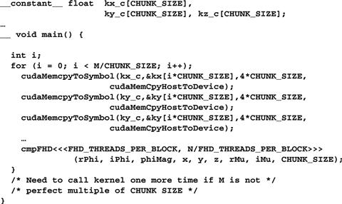
Figure 11.12 Chunking k-space data to fit into constant memory.
In Figure 11.12, the cmpFHd kernel is called from a loop. The code assumes that kx, ky, and kz arrays are in the host memory. The dimensions of kx, ky, and kz are given by M. At each iteration, the host code calls the cudaMemcpy() function to transfer a chunk of the k-space data into the device constant memory. The kernel is then invoked to process the chunk. Note that when M is not a perfect multiple of CHUNK_SIZE, the host code will need to have an additional round of cudaMemcpy() and one more kernel invocation to finish the remaining k-space data.
Figure 11.13 shows the revised kernel that accesses the k-space data from constant memory. Note that pointers to kx, ky, and kz are no longer in the parameter list of the kernel function. Since we cannot use pointers to access variables in the constant memory, the kx_c, ky_c, and kz_c arrays are accessed as global variables declared under the __constant__ keyword as shown Figure 11.12. By accessing these elements from the constant cache, the kernel now has effectively only four global memory accesses to the rMu and iMu arrays. The compiler will typically recognize that the four array accesses are made to only two locations. It will only perform two global accesses, one to rMu[m] and one to iMu[m]. The values will be stored in temporary register variables for use in the other two. This makes the final number of memory accesses two. The compute to memory access ratio is up to 13:2. This is still not quite the desired 10:1 ratio but is sufficiently high that the memory bandwidth limitation is no longer the only factor that limits performance. As we will see, we can perform a few other optimizations that make computation more efficient and further improve performance.
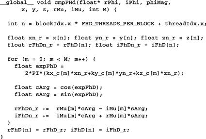
Figure 11.13 Revised FHD kernel to use constant memory.
If we ran the code in Figures 11.12 and 11.13, we would have found out that the performance enhancement was not as high as we expected for some devices. As it turns out, the code shown in these figures does not result in as much memory bandwidth reduction as we expected. The reason is that the constant cache does not perform very well for the code. This has to do with the design of the constant cache and the memory layout of the k-space data. As shown in Figure 11.14, each constant cache entry is designed to store multiple consecutive words. This design reduces the cost of constant cache hardware. If multiple data elements that are used by each thread are not in consecutive words, as illustrated in Figure 11.14(a), they will end up taking multiple cache entries. Due to cost constraints, the constant cache has only a very small number of entries. As shown in Figures 11.12 and 11.13, the k-space data is stored in three arrays: kx_c, ky_c, and kz_c. During each iteration of the loop, three entries of the constant cache are needed to hold the three k-space elements being processed. Since different warps can be at very different iterations, they may require many entries altogether. As it turns out, the constant cache capacity in some devices may not be sufficient to provide a sufficient number of entries for all the warps active in an SM.
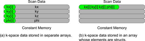
Figure 11.14 Effect of k-space data layout on constant cache efficiency: (a) k-space data stored in separate arrays, and (b) k-space data stored in an array whose elements are structs.
The problem of inefficient use of cache entries has been well studied in the literature and can be solved by adjusting the memory layout of the k-space data. The solution is illustrated in Figure 11.14(b) and the code based on this solution is shown in Figure 11.15. Rather than having the x, y, and z components of the k-space data stored in three separate arrays, the solution stores these components in an array of which the elements comprise a struct. In the literature, this style of declaration is often referred to as array of structs. The declaration of the array is shown at the top of Figure 11.15. By storing the x, y, and z components in the three fields of an array element, the developer forces these components to be stored in consecutive locations of the constant memory. Therefore, all three components used by an iteration can now fit into one cache entry, reducing the number of entries needed to support the execution of all the active warps. Note that since we have only one array to hold all k-space data, we can just use one cudaMemcpyToSymbol to copy the entire chunk to the device constant memory. The size of the transfer is adjusted from 4∗CHUNK_SIZE to 12∗CHUNK_SIZE to reflect the transfer of all the three components in one cudaMemcpy call.
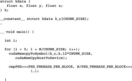
Figure 11.15 Adjusting k-space data layout to improve cache efficiency.
With the new data structure layout, we also need to revise the kernel so that the access is done according to the new layout. The new kernel is shown in Figure 11.16. Note that kx[m] has become k[m].x, ky[m] has become k[m].y, and so on. As we will see later, this small change to the code can result in significant enhancement of its execution speed.
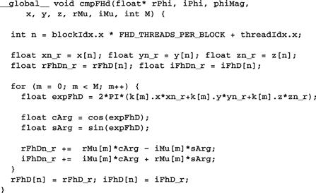
Figure 11.16 Adjusting the k-space data memory layout in the FHD kernel.
Step 3: Using Hardware Trigonometry Functions
CUDA offers hardware implementations of mathematic functions that provide much higher throughput than their software counterparts. These functions are implemented as hardware instructions executed by the SFUs (special function units). The procedure for using these functions is quite easy. In the case of the cmpFHd kernel, what we need to do is change the calls to sin() and cos() functions into their hardware versions: __sin() and __cos(). These are intrinsic functions that are recognized by the compiler and translated into SFU instructions. Because these functions are called in a heavily executed loop body, we expect that the change will result in a very significant performance improvement. The resulting cmpFHd kernel is shown in Figure 11.17.
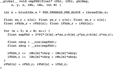
Figure 11.17 Using hardware __sin() and __cos() functions.
However, we need to be careful about the reduced accuracy when switching from software functions to hardware functions. As we discussed in Chapter 7, hardware implementations currently have slightly less accuracy than software libraries (the details are available in the CUDA Programming Guide). In the case of MRI, we need to make sure that the hardware implementation passes provide enough accuracy, as shown in Figure 11.18. The testing process involves a “perfect” image (I0). We use a reverse process to generate a corresponding “scanned” k-space data that is synthesized. The synthesized scanned data is then processed by the proposed reconstruction system to generate a reconstructed image (I). The values of the voxels in the perfect and reconstructed images are then fed into the peak signal-to-noise ratio (PSNR) formula shown in Figure 11.18.
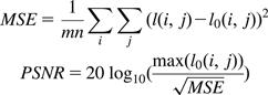
Figure 11.18 Metrics used to validate the accuracy of hardware functions. I0 is perfect image. I is reconstructed image. PSNR is Peak signal-to-noise ratio.
The criteria for passing the test depend on the application that the image is intended for. In our case, we worked with experts in clinical MRI to ensure that the PSNR changes due to hardware functions are well within the accepted limits for their applications. In applications where the images are used by physicians to form an impression of injury or evaluate a disease, one also needs to have visual inspection of the image quality. Figure 11.19 shows the visual comparison of the original “true” image. It then shows that the PSNR achieved by CPU double-precision and single-precision implementations are both 27.6 dB, an acceptable level for the application. A visual inspection also shows that the reconstructed image indeed corresponds well with the original image.
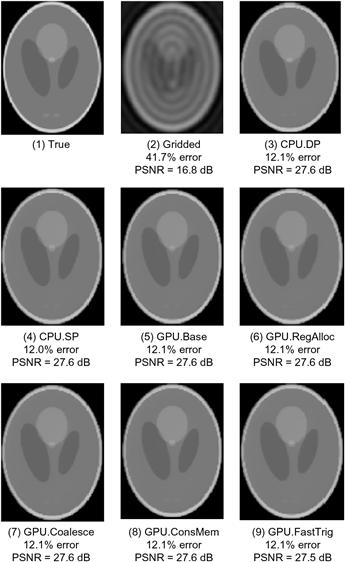
Figure 11.19 Validation of floating-point precision and accuracy of the different FHD implementations.
The advantage of iterative reconstruction compared to a simple bilinear interpolation gridding/iFFT is also obvious in Figure 11.19. The image reconstructed with the simple gridding/iFFT has a PSNR of only 16.8 dB, substantially lower than the PSNR of 27.6 dB achieved by the iterative reconstruction method. A visual inspection of the gridding/iFFT image in Figure 11.19(2) shows that there are severe artifacts that can significantly impact the usability of the image for diagnostic purposes. These artifacts do not occur in the images from the iterative reconstruction method.
When we moved from double-precision to single-precision arithmetic on the CPU, there was no measurable degradation of PSNR, which remains at 27.6 dB. When we moved the trigonometry function from the software library to the hardware units, we observed a negligible degradation of PSNR, from 27.6 dB to 27.5 dB. The slight loss of PSNR is within an acceptable range for the application. A visual inspection confirms that the reconstructed image does not have significant artifacts compared to the original image.
Step 4: Experimental Performance Tuning
Up to this point, we have not determined the appropriate values for the configuration parameters for the kernel. For example, we need to determine the optimal number of threads for each block. On one hand, using a large number of threads in a block is needed to fully utilize the thread capacity of each SM (given that 16 blocks can be assigned to each SM at maximum). On the other hand, having more threads in each block increases the register usage of each block and can reduce the number of blocks that can fit into an SM. Some possible values of number of threads per block are 32, 64, 128, 256, and 512. One could also consider non-power-of-two numbers.
Another kernel configuration parameter is the number of times one should unroll the body of the for loop. This can be set using a #pragma unroll followed by the number of unrolls we want the compiler to perform on a loop. On one hand, unrolling the loop can reduce the number of overhead instructions, and potentially reduce the number of clock cycles to process each k-space sample data. On the other hand, too much unrolling can potentially increase the usage of registers and reduce the number of blocks that can fit into an SM.
Note that the effects of these configurations are not isolated from each other. Increasing one parameter value can potentially use the resource that could be used to increase another parameter value. As a result, one needs to evaluate these parameters jointly in an experimental manner. That is, one may need to change the source code for each joint configuration and measure the runtime. There can be a large number of source code versions to try. In the case of FHD, the performance improves about 20% by systematically searching all the combinations and choosing the one with the best measured runtime, as compared to a heuristic tuning search effort that only explores some promising trends. Ryoo et al. present a pareto optimal curve–based method to screen away most of the inferior combinations [RRS2008].
11.4 Final Evaluation
To obtain a reasonable baseline, we implemented two versions of FHD on the CPU. Version CPU.DP uses double precision for all floating-point values and operations, while version CPU.SP uses single precision. Both CPU versions are compiled with Intel’s ICC (version 10.1) using flags -O3 -msse3 -axT -vec-report3 -fp-model fast=2, which (1) vectorizes the algorithm’s dominant loops using instructions tuned for the Core 2 architecture, and (2) links the trigonometric operations to fast, approximate functions in the math library. Based on experimental tuning with a smaller data set, the inner loops are unrolled by a factor of four and the scan data is tiled to improve locality in the L1 cache.
Each GPU version of FHD is compiled using NVCC-O3 (CUDA version 1.1) and executed on a 1.35 GHz Quadro FX5600. The Quadro card is housed in a system with a 2.4 GHz dual-socket, dual-core Opteron 2216 CPU. Each core has a 1 MB L2 cache. The CPU versions use p-threads to execute on all four cores of a 2.66 GHz Core 2 Extreme quad-core CPU, which has peak theoretical capacity of 21.2 GFLOPS per core and a 4 MB L2 cache. The CPU versions perform substantially better on the Core 2 Extreme quad-core than on the dual-socket, dual-core Opteron. Therefore, we will use the Core 2 Extreme quad-core results for the CPU.
All reconstructions use the CPU version of the linear solver, which executes 60 iterations on the Quadro FX5600. Two versions of Q were computed on the Core 2 Extreme, one using double precision and the other using single precision. The single-precision Q was used for all GPU-based reconstructions and for the reconstruction involving CPU.SP, while the double-precision Q was used only for the reconstruction involving CPU.DP. As the computation of Q is not on the reconstruction’s critical path, we give Q no further consideration.
To facilitate comparison of the iterative reconstruction with a conventional reconstruction, we also evaluated a reconstruction based on bilinear interpolation gridding and inverse FFT. Our version of the gridded reconstruction is not optimized for performance, but it is already quite fast.
All reconstructions are performed on sample data obtained from a simulated, 3D, non-Cartesian scan of a phantom image. There are 284,592 sample points in the scan data set, and the image is reconstructed at 1,283 resolution, for a total of 221 voxels. In the first set of experiments, the simulated data contains no noise. In the second set of experiments, we added complex white Gaussian noise to the simulated data. When determining the quality of the reconstructed images, the percent error and PSNR metrics are used. The percent error is the root-mean-square (RMS) of the voxel error divided by the RMS voxel value in the true image (after the true image has been sampled at 1,283 resolution).
The data (runtime, GFLOPS, and images) was obtained by reconstructing each image once with each of the implementations of the FHD algorithm described before. There are two exceptions to this policy. For GPU.Tune and GPU.Multi, the time required to compute FHD is so small that runtime variations in performance became non-negligible. Therefore, for these configurations we computed FHD three times and reported the average performance.
As shown in Figure 11.20, the total reconstruction time for the test image using bilinear interpolation gridding followed by inverse FFT takes less than one minute on a high-end sequential CPU. This confirms that there is little value in parallelizing this traditional reconstruction strategy. It is, however, obvious from Figure 11.19(2) that the resulting image exhibits an unacceptable level of artifacts.
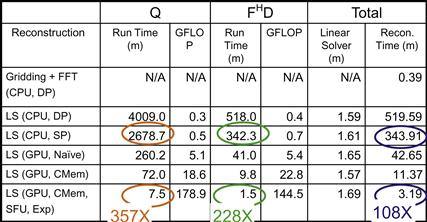
Figure 11.20 Summary of performance improvements.
The LS (CPU, DP) row shows the execution timing of reconstructing the test image using double-precision, floating-point arithmetic on the CPU. The timing shows the core step (Q) of calculating FHF+λWHW. The first observation is that the Q computation for a moderate resolution image based on a moderate-size data sample takes an unacceptable amount of time (more than 65 hours) on the CPU for setting up the system for a patient. Note that this time is eventually reduced to 6.5 minutes on the GPU with all the optimizations described in Section 11.3. The second observation is that the total reconstruction time of each image requires more than 8 hours, with only 1.59 minutes spent in the linear solver. This validates our decision to focus our parallelization effort on FHD.
The LS (CPU, SP) row shows that we can reduce the execution time significantly when we convert the computation from double-precision, floating-point arithmetic to single precision on the CPU. This is because the streaming SIMD instruction (SSE) instructions have higher throughput, that is, they calculate more data elements per clock cycle when executing in single-precision mode. The execution times, however, are still unacceptable for practical use.
The LS (GPU, Naïve) row shows that a straightforward CUDA implementation can achieve a speedup about 10× for Q and 8× for the reconstruction of each image. This is a good speedup, but the resulting execution times are still unacceptable for practical use.
The LS (GPU, CMem) row shows that significant further speedup is achieved by using registers and constant cache to get around the global memory bandwidth limitations. These enhancements achieve about 4× speedup over the naïve CUDA code! This shows the importance of achieving optimal compute to memory ratios in CUDA kernels. These enhancements bring the CUDA code to about 40× speedup over the single-precision CPU code.
The LS (GPU, CMem, SPU, Exp) row shows the use of hardware trigonometry functions and experimental tuning together, and results in a dramatic speedup. A separate experiment, not shown in the figure, shows that most of the speedup comes from hardware trigonometry functions. The total speedup over CPU single-precision code is very impressive: 357× for Q and 108× for the reconstruction of each image.
An interesting observation is that in the end, the linear solver actually takes more time than FHD. This is because we have accelerated FHD dramatically (228×). What used to be close to 100% of the per-image reconstruction time now accounts for less than 50%. Any further acceleration will now require acceleration of the linear solver, a much more difficult type of computation for massively parallel execution.
11.5 Exercises
11.1. Loop fission splits a loop into two loops. Use the FHD code in Figure 11.4(b) and enumerate the execution order of the two parts of the outer loop body: (1) the statements before the inner loop and (2) the inner loop.
(a) List the execution order of these parts from different iterations of the outer loop before fission.
(b) List the execution order of these parts from the two loops after fission. Determine if the execution results will be identical. The execution results are identical if all data required by a part is properly generated and preserved for its consumption before that part executes, and the execution result of the part is not overwritten by other parts that should come after the part in the original execution order.
11.2. Loop interchange swaps the inner loop into the outer loop and vice versa. Use the loops from Figure 11.9 and enumerate the execution order of the instances of the loop body before and after the loop exchange.
(a) List the execution order of the loop body from different iterations before the loop interchange. Identify these iterations with the values of m and n.
(b) List the execution order of the loop body from different iterations after the loop interchange. Identify these iterations with the values of m and n.
(c) Determine if the (a) and (b) execution results will be identical. The execution results are identical if all data required by a part is properly generated and preserved for its consumption before that part executes and the execution result of the part is not overwritten by other parts that should come after the part in the original execution order.
11.3. In Figure 11.11, identify the difference between the access to x[] and kx[] in the nature of indices used. Use the difference to explain why it does not make sense to try to load kx[n] into a register for the kernel shown in Figure 11.11.
11.4. During a meeting, a new graduate student told his advisor that he improved his kernel performance by using cudaMalloc() to allocate constant memory and by using cudaMemcpy() to transfer read-only data from the CPU memory to the constant memory. If you were his advisor, what would be your response?
References
1. Liang ZP, Lauterbur P. Principles of Magnetic Resonance Imaging: A Signal Processing Perspective New York: John Wiley and Sons; 1999.
2. Haldar JP, Hernando D, Budde MD, Wang Q, Song S-K, Liang. Z-P. High-resolution MR metabolic imaging. In Proc IEEE EMBS 2007:4324–4326.
3. Ryoo S, Ridrigues CI, Stone SS, et al. Program optimization carving for GPU computing. Journal of Parallel and Distributed Computing 2008;. doi 10.1016/j.jpdc.2008.05.011.
4. S. S. Stone, J. P. Haldar, S. C. Tsao, W. W. Hwu, B. P. Sutton, and Z. P. Liang, Accelerating advanced MRI reconstruction on GPUs, Journal of Parallel and Distributed Computing, 2008, doi:10.1016/j.jpdc.2008.05.013.
1Note that the FHD computation can be approximated with gridding and can run in a few seconds, with perhaps reduced quality of the final reconstructed image.
2Note that declaring x[], y[], z[], rFhD[], and iFhD[] as automatic arrays will not work for our purpose here. Such declaration would have created private copies of all these five arrays in the local memory of every thread! All we want is to have a private copy of one element of each array in the registers of each thread.
3The reason why a constant memory access is not exactly as efficient as a register access is that a memory load instruction is still needed for access to the constant memory.
4Note not all accesses to read-only data are as favorable for constant memory as what we have here. In Chapter 12 we present a case where threads in different blocks access different elements in the same iteration. This more diverged access pattern makes it much harder to fit enough of the data into the constant memory for a kernel launch.