Basic Manipulations and Properties

A column vector x with d dimensions can be written

$\mathbf{x}\equiv \left[\begin{array}{c}{x}_1\\ x_2\\ ⋮\\ x_d\end{array}\right]={\left[\begin{array}{cccc}{x}_1& x_2& \cdots & x_d\end{array}\right]}^T,$

where the transpose operator, superscript T, allows it be written as a transposed row vector—which is useful when defining vectors in running text. In this book, vectors are assumed to be row vectors.

The transpose A^T of a matrix A involves copying all the rows of the original matrix A into the columns of A^T. Thus a matrix with m rows and n columns becomes a matrix with n rows and m columns:

$\begin{array}{ccc}\mathbf{A}\equiv \left[\begin{array}{cccc}{a}_{11}& a_{12}& \cdots & a_{1n}\\ a_{21}& a_{21}& \cdots & a_{2n}\\ ⋮& ⋮& \ddots & ⋮\\ a_{m1}& a_{m2}& \cdots & a_{mn}\end{array}\right]& \Rightarrow & {\mathbf{A}}^{\mathit{T}}=\left[\begin{array}{cccc}{a}_{11}& a_{21}& \cdots & a_{m1}\\ a_{12}& a_{21}& \cdots & a_{m2}\\ ⋮& ⋮& \ddots & ⋮\\ a_{1n}& a_{2n}& \cdots & a_{nm}\end{array}\right]\end{array}.$

The dot product or inner product between vector x and vector y of the same dimensionality yields a scalar quantity,

$\mathbf{x}·\mathbf{y}=⟨\mathbf{x},\mathbf{y}⟩={\mathbf{x}}^T\mathbf{y}=\sum _{i=1}^D{x}_i{y}_i.$

For example, the Euclidean norm can be written as the square root of the dot product of a vector x with itself, $\left|\right|\mathbf{x}|{|}_2=\sqrt{{\mathbf{x}}^T\mathbf{x}}$.

The tensor product or outer product ⊗ between an m-dimensional vector x and an n-dimensional vector y yields a matrix,

$\mathbf{x}\otimes \mathbf{y}\equiv \mathbf{x}{\mathbf{y}}^T=\left[\begin{array}{c}{x}_1\\ x_2\\ ⋮\\ x_m\end{array}\right][\begin{array}{cccc}{y}_1& y_2& \cdots & y_n\end{array}]=\left[\begin{array}{cccc}{x}_1{y}_1& x_1{y}_2& \cdots & x_1{y}_n\\ x_2{y}_1& x_2{y}_2& \cdots & x_2{y}_n\\ ⋮& ⋮& \ddots & ⋮\\ x_m{y}_1& x_m{y}_2& \cdots & x_m{y}_n\end{array}\right]$

Given an N row and K column matrix A, and a K row and M column matrix B, if we write each row of A as ${\mathbf{a}}_n^T$ and each column of B as b_m, the matrix product AB (i.e., matrix multiplication) can be written

$\mathbf{A}\mathbf{B}=\left[\begin{array}{c}{\mathbf{a}}_1^T\\ {\mathbf{a}}_2^T\\ ⋮\\ {\mathbf{a}}_N^T\end{array}\right][\begin{array}{cccc}{\mathbf{b}}_1& {\mathbf{b}}_2& \cdots & {\mathbf{b}}_M\end{array}]=\left[\begin{array}{cccc}{\mathbf{a}}_1^T{\mathbf{b}}_1& {\mathbf{a}}_1^T{\mathbf{b}}_2& \cdots & {\mathbf{a}}_1^T{\mathbf{b}}_M\\ {\mathbf{a}}_2^T{\mathbf{b}}_1& {\mathbf{a}}_2^T{\mathbf{b}}_2& \cdots & {\mathbf{a}}_2^T{\mathbf{b}}_M\\ ⋮& ⋮& \ddots & ⋮\\ {\mathbf{a}}_N^T{\mathbf{b}}_1& {\mathbf{a}}_N^T{\mathbf{b}}_2& \cdots & {\mathbf{a}}_N^T{\mathbf{b}}_M\end{array}\right].$

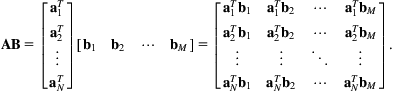
If we write each column of A as a_k and each row of B as ${\mathbf{b}}_k^T$, the matrix product AB can also be written in terms of tensor products

$\mathbf{A}\mathbf{B}=[\begin{array}{cccc}{\mathbf{a}}_1& {\mathbf{a}}_2& \cdots & {\mathbf{a}}_K\end{array}]\left[\begin{array}{c}{\mathbf{b}}_1^T\\ {\mathbf{b}}_2^T\\ ⋮\\ {\mathbf{b}}_K^T\end{array}\right]=\sum _{k=1}^K{\mathbf{a}}_k{\mathbf{b}}_k^T.$

The elementwise product or Hadamard product of two matrices that are of the same size is

$\begin{array}{ll}\mathbf{A}\circ \mathbf{B}\hfill & =\left[\begin{array}{cccc}{a}_{11}& a_{12}& \cdots & a_{1n}\\ a_{21}& a_{21}& \cdots & a_{2n}\\ ⋮& ⋮& \ddots & ⋮\\ a_{m1}& a_{m2}& \cdots & a_{mn}\end{array}\right]\circ \left[\begin{array}{cccc}{b}_{11}& b_{12}& \cdots & b_{1n}\\ b_{21}& b_{21}& \cdots & b_{2n}\\ ⋮& ⋮& \ddots & ⋮\\ b_{m1}& b_{m2}& \cdots & b_{mn}\end{array}\right]\hfill \\ \hfill & =\left[\begin{array}{cccc}{a}_{11}{b}_{11}& a_{12}{b}_{12}& \cdots & a_{1n}{b}_{1n}\\ a_{211}{b}_{21}& b_{21}{b}_{21}& \cdots & a_{2n}{b}_{2n}\\ ⋮& ⋮& \ddots & ⋮\\ a_{m1}{b}_{m1}& a_{m2}{b}_{m2}& \cdots & a_{mn}{b}_{mn}\end{array}\right].\hfill \end{array}$

A square matrix A with n rows and n columns is invertible if there exists a square matrix B=A⁻¹ such that AB=BA=I, where I is the identity matrix consisting of all zeros except that all diagonal elements are one. Square matrices that are not invertible are called singular. A square matrix A is singular if and only if its determinant, det(A), is zero. The following equation for the inverse shows why a zero determinant implies that a matrix is not invertible:

${\mathbf{A}}^{-1}=\frac{1}{\det (\mathbf{A})}{\mathbf{C}}^T,$

where det(A) is the determinant of A and C is another matrix known as the cofactor matrix. Finally, if a matrix A is orthogonal, then A⁻¹=A^T.

Derivatives of Vector and Scalar Functions

Given a scalar function y of an m-dimensional column vector x,

$\frac{\partial y}{\partial \mathbf{x}}\equiv \left[\begin{array}{c}\frac{\partial y}{\partial x_1}\\ \frac{\partial y}{\partial x_2}\\ ⋮\\ \frac{\partial y_1}{\partial x_m}\end{array}\right]=\mathbf{g}.$

This quantity is known as the gradient, g. We have defined it here as a column vector, but it is sometimes defined as a row vector. Defining the gradient as a column vector implies certain orientations for the other quantities defined below, so keep in mind that the derivatives that follow are sometimes defined as the transposes of those given here. Using the definition and orientation above we can write the types of parameter updates frequently used in algorithms like gradient descent in vector form with expressions such as ${\mathbf{\theta }}^{\mathrm{new}}={\mathbf{\theta }}^{\mathrm{old}}-\mathbf{g}$, where θ is a parameter (column) vector.

Given a scalar x and n-dimensional vector function y,

$\frac{\partial \mathbf{y}}{\partial x}\equiv \left[\begin{array}{cccc}\frac{\partial y_1}{\partial x}& \frac{\partial y_2}{\partial x}& \cdots & \frac{\partial y_n}{\partial x}\end{array}\right].$

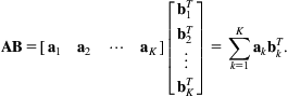
For an m-dimensional vector x and an n-dimensional vector y, the Jacobian matrix is given by

$\frac{\partial \mathbf{y}}{\partial \mathbf{x}}\equiv \left[\begin{array}{cccc}\frac{\partial y_1}{\partial x_1}& \frac{\partial y_2}{\partial x_1}& \cdots & \frac{\partial y_n}{\partial x_1}\\ \frac{\partial y_1}{\partial x_2}& \frac{\partial y_2}{\partial x_2}& \cdots & \frac{\partial y_n}{\partial x_2}\\ ⋮& ⋮& \ddots & ⋮\\ \frac{\partial y_1}{\partial x_m}& \frac{\partial y_2}{\partial x_m}& \cdots & \frac{\partial y_n}{\partial x_m}\end{array}\right].$

The Jacobian is sometimes defined as the transpose of this quantitiy even given the other definitions above. Watch out for the implications. The derivative of a scalar function y=f(X) with respect to an m×n dimensional matrix X is known as a gradient matrix and is given by

$\frac{\partial f}{\partial \mathbf{X}}\equiv \left[\begin{array}{cccc}\frac{\partial y}{\partial x_{11}}& \frac{\partial y}{\partial x_{12}}& \cdots & \frac{\partial y}{\partial x_{1n}}\\ \frac{\partial y}{\partial x_{21}}& \frac{\partial y}{\partial x_{22}}& \cdots & \frac{\partial y}{\partial x_{2n}}\\ ⋮& ⋮& \ddots & ⋮\\ \frac{\partial y}{\partial x_{m1}}& \frac{\partial y}{\partial x_{m2}}& \cdots & \frac{\partial y}{\partial x_{mn}}\end{array}\right]=\mathbf{G}.$

Our choice for the orientations of these quantities means that the gradient matrix has the same layout as the original matrix, so updates to a parameter matrix X take the form ${\mathbf{X}}^{\mathrm{new}}={\mathbf{X}}^{\mathrm{old}}-\mathbf{G}$.

While many quantities can be expressed as scalars, vectors, or matrices, there are many that cannot. Inspired by the tabular visualization of Minka (2000), the scalar, vector, matrix, and tensor quantities resulting from taking the derivatives of different combinations of quantities are shown in Table A.1.

Table A.1

Quantities That Result From Various Derivatives (After Minka, 2000)

	Scalar $\frac{\partial f}{\cdot }$	Vector $\frac{\partial \mathbf{f}}{\cdot }$	Matrix $\frac{\partial \mathbf{F}}{\cdot }$
Scalar $\frac{\cdot }{\partial x}$	Scalar: $\frac{\partial f}{\partial x}=g$	Vector: $\frac{\partial \mathbf{f}}{\partial x}\equiv \left[\frac{\partial f_i}{\partial x}\right]={\mathbf{g}}^T$	Matrix: $\frac{\partial \mathbf{F}}{\partial x}\equiv \left[\frac{\partial f_{ij}}{\partial x}\right]={\mathbf{G}}^T$
Vector $\frac{\cdot }{\partial \mathbf{x}}$	Vector: $\frac{\partial f}{\partial \mathbf{x}}\equiv \left[\frac{\partial f}{\partial x_i}\right]=\mathbf{g}$	Matrix: $\frac{\partial \mathbf{f}}{\partial \mathbf{x}}\equiv \left[\frac{\partial f_i}{\partial x_j}\right]=\mathbf{G}$	Tensor: $\frac{\partial \mathbf{F}}{\partial \mathbf{x}}\equiv \left[\frac{\partial {\mathbf{F}}_{ij}}{\partial x_k}\right]$
Matrix $\frac{\cdot }{\partial \mathbf{X}}$	Matrix: $\frac{\partial f}{\partial \mathbf{X}}\equiv \left[\frac{\partial f}{\partial x_{ij}}\right]=\mathbf{G}$	Tensor: $\frac{\partial \mathbf{f}}{\partial \mathbf{X}}\equiv \left[\frac{\partial f_i}{\partial x_{jk}}\right]$	Tensor: $\frac{\partial \mathbf{F}}{\partial \mathbf{X}}\equiv \left[\frac{\partial f_{ij}}{\partial x_{kl}}\right]$

The Chain Rule

The chain rule for a function z, which is a function of y, which is a function of x, all of which are scalars, is

$\frac{\partial z}{\partial x}=\frac{\partial z}{\partial y}\frac{\partial y}{\partial x}$

where the two terms could be reversed, because multiplication is commutative. Now, given an m-dimensional vector x, an n-dimensional vector y, and an o-dimensional vector z, if z=z(y(x)), then

$\frac{\partial \mathbf{z}}{\partial \mathbf{x}}\equiv \left[\begin{array}{cccc}\frac{\partial z_1}{\partial x_1}& \frac{\partial z_2}{\partial x_1}& \cdots & \frac{\partial z_o}{\partial x_1}\\ \frac{\partial z_1}{\partial x_2}& \frac{\partial z_2}{\partial x_2}& \cdots & \frac{\partial z_o}{\partial x_2}\\ ⋮& ⋮& \ddots & ⋮\\ \frac{\partial z_1}{\partial x_m}& \frac{\partial z_2}{\partial x_m}& \cdots & \frac{\partial z_o}{\partial x_m}\end{array}\right],$

where each entry in the m×n matrix can be computed using

$\frac{\partial z_i}{\partial x_j}=\sum _{k=1}^n\frac{\partial y_k}{\partial x_j}\frac{\partial z_i}{\partial y_k}=\left[\frac{\partial \mathbf{y}}{\partial x_j}\right]\left[\frac{\partial z_i}{\partial \mathbf{y}}\right].$

The vector form could be viewed as

$\begin{array}{ll}\frac{\partial \mathbf{z}}{\partial \mathbf{x}}\hfill & =\left[\begin{array}{cccc}\frac{\partial y_1}{\partial x_1}& \frac{\partial y_2}{\partial x_1}& \cdots & \frac{\partial y_n}{\partial x_1}\\ \frac{\partial y_1}{\partial x_2}& \frac{\partial y_2}{\partial x_2}& \cdots & \frac{\partial y_n}{\partial x_2}\\ ⋮& ⋮& \ddots & ⋮\\ \frac{\partial y_1}{\partial x_m}& \frac{\partial y_2}{\partial x_m}& \cdots & \frac{\partial y_n}{\partial x_m}\end{array}\right]\left[\begin{array}{cccc}\frac{\partial z_1}{\partial y_1}& \frac{\partial z_2}{\partial y_1}& \cdots & \frac{\partial z_o}{\partial y_1}\\ \frac{\partial z_1}{\partial y_2}& \frac{\partial z_2}{\partial y_2}& \cdots & \frac{\partial z_o}{\partial y_2}\\ ⋮& ⋮& \ddots & ⋮\\ \frac{\partial z_1}{\partial y_n}& \frac{\partial z_2}{\partial y_n}& \cdots & \frac{\partial z_o}{\partial y_n}\end{array}\right]\hfill \\ \frac{\partial \mathbf{z}}{\partial \mathbf{x}}\hfill & =\frac{\partial \mathbf{y}}{\partial \mathbf{x}}\frac{\partial \mathbf{z}}{\partial \mathbf{y}},\hfill \end{array}$

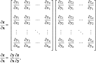
which yields the chain rule for vectors, where chains extend toward the left as opposed to the right as is often done with the scalar version. For the special case when the final function evaluates to a scalar—which is frequently encountered when optimizing a loss function, we have

$\begin{array}{ll}\frac{\partial z}{\partial x_j}\hfill & =\sum _{k=1}^n\frac{\partial y_k}{\partial x_j}\frac{\partial z}{\partial y_k},\hfill \\ \frac{\partial z}{\partial \mathbf{x}}\hfill & =\frac{\partial \mathbf{y}}{\partial \mathbf{x}}\frac{\partial z}{\partial \mathbf{y}}.\hfill \end{array}$

The rule generalizes, so that if there were yet another vector function w that is a function of x, through z, then

$\frac{\partial \mathbf{w}}{\partial \mathbf{x}}=\frac{\partial \mathbf{y}}{\partial \mathbf{x}}\frac{\partial \mathbf{z}}{\partial \mathbf{y}}\frac{\partial \mathbf{w}}{\partial \mathbf{z}}.$

To find the derivative of a matrix that is the function of another matrix, the chain rule generalizes. For example, for a matrix X if matrix Y=f(X), the derivative of a function g(Y) is

$\begin{array}{ll}\frac{\partial g(\mathbf{Y})}{\partial \mathbf{X}}\hfill & =\frac{\partial g(f(\mathbf{X}))}{\partial \mathbf{X}}\hfill \\ \frac{\partial g(\mathbf{Y})}{\partial x_{ij}}\hfill & =\sum _{k=1}^K\sum _{l=1}^L\frac{\partial g(\mathbf{Y})}{\partial y_{kl}}\frac{\partial y_{kl}}{\partial x_{ij}}\hfill \end{array}$

Computation Graphs and Backpropagation

Computation networks help to show how the gradients required for deep learning with backpropagation can be computed. They also provide the basis for many software packages for deep learning, which partially or fully automate the computations involved.

We begin with an example that computes intermediate quantities that are scalars, and then extend it to networks involving vectors that represent entire layers of variables at each node. Fig. A.1 gives a computation graph that implements the function z₁(y₁,z₂(y₂(y₁),z₃(y₃(y₂(y₁))))), and shows how to compute the gradients. The chain rule for a scalar function a involving intermediate results b₁,…,b_k that are dependent on c is

$\frac{\partial a(b_1,\dots ,b_k)}{\partial c}=\sum _{k=1}^n\frac{\partial a}{\partial b_k}\frac{\partial b_k}{\partial c}.$

In the example, the partial derivative of z₁ with respect to y₁ therefore consists of three terms

$\begin{array}{ll}\frac{\partial z_1}{\partial y_1}\hfill & =\underset{(1)}{\underbrace{\frac{\partial z_1}{\partial y_1}}}+\underset{(2)}{\underbrace{\frac{\partial z_1}{\partial z_2}\frac{\partial z_2}{\partial y_2}\frac{\partial y_2}{\partial y_1}}}+\underset{(3)}{\underbrace{\frac{\partial z_1}{\partial z_2}\frac{\partial z_2}{\partial z_3}\frac{\partial z_3}{\partial y_3}\frac{\partial y_3}{\partial y_2}\frac{\partial y_2}{\partial y_1}}}\hfill \\ \hfill & =\frac{\partial z_1}{\partial y_1}+\frac{\partial z_1}{\partial z_2}\left[\frac{\partial z_2}{\partial y_2}+\frac{\partial z_2}{\partial z_3}\frac{\partial z_3}{\partial y_3}\frac{\partial y_3}{\partial y_2}\right]\frac{\partial y_2}{\partial y_1}\hfill \end{array}$

The sums needed to compute this involve following back along the flows of the subcomputations that were performed to evaluate the original function. These can be implemented efficiently by passing them between nodes in the graph, as Fig. A.1 shows.

This high-level notion of following flows in a graph generalizes to deep networks involving entire layers of variables. If Fig. A.1 were drawn using a scalar for z₁ and vectors for each of the other nodes, the partial derivatives could be replaced by their vector versions. It is necessary to reverse the order of the multiplications, because in the case of partial derivatives of vectors with respect to vectors, computations grow to the left, yielding

$\frac{\partial z_1}{\partial {\mathbf{y}}_1}=\frac{\partial z_1}{\partial {\mathbf{y}}_1}+\frac{\partial {\mathbf{y}}_2}{\partial {\mathbf{y}}_1}\left[\frac{\partial {\mathbf{z}}_2}{\partial {\mathbf{y}}_2}+\frac{\partial {\mathbf{y}}_3}{\partial {\mathbf{y}}_2}\frac{\partial {\mathbf{z}}_3}{\partial {\mathbf{y}}_3}\frac{\partial {\mathbf{z}}_2}{\partial {\mathbf{z}}_3}\right]\frac{\partial z_1}{\partial {\mathbf{z}}_2}$

To see this, consider (1) the chain rule for the partial derivative of a scalar function z with a vector x as argument, but involving the computation of an intermediate vector y:

$\begin{array}{ll}\hfill \frac{\partial z(\mathbf{y})}{\partial x_j}& =\sum _{k=1}^n\frac{\partial y_k}{\partial x_j}\frac{\partial z}{\partial y_k}\hfill \\ \hfill \frac{\partial z}{\partial \mathbf{x}}& =\frac{\partial \mathbf{y}}{\partial \mathbf{x}}\frac{\partial z}{\partial \mathbf{y}}\hfill \\ \hfill & =\mathbf{D}\mathbf{d},\hfill \end{array}$

and (2) the chain rule for the same scalar function z(x), but involving the computation of an intermediate matrix Y:

$\begin{array}{ll}\frac{\partial z(\mathbf{Y})}{\partial \mathbf{x}}\hfill & =\sum _{l=1}^L\frac{\partial {\mathbf{y}}_l}{\partial \mathbf{x}}\frac{\partial z}{\partial {\mathbf{y}}_l}\hfill \\ \hfill & =\sum _{l=1}^L{\mathbf{D}}_l{\mathbf{d}}_l.\hfill \end{array}$

Derivatives of Functions of Vectors and Matrices

Here are some useful derivatives for functions of vectors and matrices. Petersen and Pedersen (2012) gives an even larger list.

$\begin{array}{l}\frac{\partial }{\partial \mathbf{x}}\mathbf{A}\mathbf{x}={\mathbf{A}}^T\hfill \\ \frac{\partial }{\partial \mathbf{x}}{\mathbf{x}}^T\mathbf{x}=2\mathbf{x}\hfill \\ \frac{\partial }{\partial \mathbf{a}}{\mathbf{a}}^T\mathbf{x}=\frac{\partial }{\partial \mathbf{a}}{\mathbf{x}}^T\mathbf{a}=\mathbf{x}\hfill \\ \frac{\partial }{\partial \mathbf{x}}{\mathbf{x}}^T\mathbf{A}\mathbf{x}=\mathbf{A}\mathbf{x}+{\mathbf{A}}^T\mathbf{x}\hfill \\ \frac{\partial }{\partial \mathbf{A}}{\mathbf{y}}^T\mathbf{A}\mathbf{x}=\mathbf{y}{\mathbf{x}}^T\hfill \\ \frac{\partial }{\partial \mathbf{x}}{(\mathbf{a}-\mathbf{x})}^T(\mathbf{a}-\mathbf{x})=-2(\mathbf{a}-\mathbf{x})\hfill \end{array}$

Notice that the first identity above would be equal to simply A, had we defined the Jacobian to be the transpose of our definition above.

For a symmetric matrix C (e.g., an inverse covariance matrix),

$\begin{array}{l}\frac{\partial }{\partial \mathbf{a}}{(\mathbf{a}-\mathbf{b})}^T\mathbf{C}(\mathbf{a}-\mathbf{b})=2\mathbf{C}(\mathbf{a}-\mathbf{b})\hfill \\ \frac{\partial }{\partial \mathbf{b}}{(\mathbf{a}-\mathbf{b})}^T\mathbf{C}(\mathbf{a}-\mathbf{b})=-2\mathbf{C}(\mathbf{a}-\mathbf{b})\hfill \\ \frac{\partial }{\partial \mathbf{w}}{(\mathbf{y}-\mathbf{A}\mathbf{w})}^T\mathbf{C}(\mathbf{y}-\mathbf{A}\mathbf{w})=-2{\mathbf{A}}^T\mathbf{C}(\mathbf{y}-\mathbf{A}\mathbf{w})\hfill \end{array}$

Vector Taylor Series Expansion, Second-Order Methods, and Learning Rates

The method of gradient descent, the interpretation of learning rates, and more sophisticated second-order methods can be viewed through the lens of the Taylor series expansion of a function. The approach presented below is also known as Newton’s method.

The Taylor expansion of a function near point x_o can be written

$f(x)=f(x_o)+\frac{f\prime (x_o)}{1!}(x-x_o)+\frac{f″(x_o)}{2!}{(x-x_o)}^2+\frac{f^{(3)}(x_o)}{3!}{(x-x_o)}^3+\cdots$

Using the approximation up to the second-order (squared) terms in x, taking the derivative, setting the result to zero, and solving for x, gives

$\begin{array}{ll}0\hfill & =\frac{d}{dx}\left[f(x_o)+f\prime (x_o)(x-x_o)+\frac{f″(x_o)}{2}{(x-x_o)}^2\right]\hfill \\ \hfill & =f\prime (x_o)+f″(x_o)(x-x_o),\mathrm{thus}\mathrm{solving}\mathrm{for}\delta x\equiv (x-x_o)\hfill \\ \hfill & \Rightarrow \delta x=-\frac{f\prime (x_o)}{f″(x_o)},\mathrm{or}x=x_o-\frac{f\prime (x_o)}{f″(x_o)}.\hfill \end{array}$

This generalizes to the vector version of a Taylor series for a scalar function with matrix arguments, where

$\begin{array}{l}f(\mathbf{\theta })=f({\mathbf{\theta }}_o)+{\mathbf{g}}_o^T(\mathbf{\theta }-{\mathbf{\theta }}_o)+\frac{1}{2}{(\mathbf{\theta }-{\mathbf{\theta }}_o)}^T{\mathbf{H}}_o(\mathbf{\theta }-{\mathbf{\theta }}_o)+\cdots ,\hfill \\ {\mathbf{g}}_o=\frac{df}{d{\mathbf{\theta }}_o},{\mathbf{H}}_o=\frac{d}{d{\mathbf{\theta }}_o}\frac{df}{d{\mathbf{\theta }}_o}=\frac{d^{2}f}{d{\mathbf{\theta }}_o^2}.\hfill \end{array}$

Using the identities given in the previous section, taking the derivative with respect to the parameter vector θ, setting it to zero and then solving for the point at which the quadratic approximation to the function would be zero, yields

$\begin{array}{ll}\frac{df(\mathbf{\theta })}{d\mathbf{\theta }}\hfill & =0={\mathbf{g}}_o+{\mathbf{H}}_o(\mathbf{\theta }-{\mathbf{\theta }}_o),\mathrm{\Delta }\mathbf{\theta }\equiv (\mathbf{\theta }-{\mathbf{\theta }}_o)\hfill \\ \Rightarrow \mathrm{\Delta }\mathbf{\theta }\hfill & =-{\mathbf{H}}_o^{-1}{\mathbf{g}}_o.\hfill \end{array}$

This means that for the update ${\mathbf{\theta }}^{\mathrm{new}}={\mathbf{\theta }}_o-{\mathbf{H}}_o^{-1}{\mathbf{g}}_o$, the learning rate used for gradient descent can be thought of in terms of a simple diagonal matrix approximation to the inverse Hessian matrix in a second-order method. In other words, using a simple learning rate is analogous to making an approximation, so that ${\mathbf{H}}_o^{-1}=\eta \mathbf{I}$.

Full-blown second-order methods take more effective steps at each iteration. However, they can be expensive because of the need to compute this quantity. For convex problems like logistic regression, a popular second-order method known as L-BFGS builds an approximation to the Hessian. Here, L stands for limited memory and BFGS stands for the inventors of the approach, Broyden–Fletcher–Goldfarb–Shanno. Another family of approaches are known as the conjugate gradient algorithms and involve working with the linear system of equations associated with ${\mathbf{H}}_o\mathbf{x}\mathbf{=}\mathbf{-}{\mathbf{g}}_o$ when solving for $\mathbf{x}=\mathrm{\Delta }\mathbf{\theta }$ as opposed to computing the inverse of ${\mathbf{H}}_o$.

One needs to keep in mind that when solving nonconvex problems (e.g., learning for multilayer neural networks) the Hessian is not guaranteed to be positive definite, which means that it may not even be invertible. Consequently the use of heuristic adaptive learning rates and momentum terms remain popular and effective for neural network methods.

Eigenvectors, Eigenvalues, and Covariance Matrices

There is a strong connection between eigenvectors, eigenvalues and diagonalization of a covariance matrix, and the method of principal component analysis. If λ is a scalar eigenvalue of a matrix A, there exists a vector x called an eigenvector of A such that Ax=λx. Define a matrix Φ to consist of eigenvectors in each column, and define Λ as a matrix with the corresponding eigenvalues on the diagonal, then the matrix equation $\mathbf{{\rm A}}\mathbf{\Phi }=\mathbf{\Phi }\mathrm{\Lambda }$ defines the eigenvalues and eigenvectors of A.

Many numerical linear algebra software packages (e.g., Matlab) can determine solutions to this equation. If the eigenvectors in Φ are orthogonal, which they are for symmetric matrices, the inverse of Φ equals its transpose, which implies that we could equally well write ${\mathbf{\Phi }}^T\mathbf{{\rm A}}\mathbf{\Phi }=\mathrm{\Lambda }$. To find the eigenvectors of a covariance matrix, set A=Σ, the covariance matrix. This yields the definition of the eigenvectors of a covariance matrix Σ as the set of orthogonal vectors stored in a matrix Φ and normalized to have unit length, such that ${\mathbf{\Phi }}^T\mathbf{\Sigma }\mathbf{\Phi }=\mathrm{\Lambda }$. Since Λ is diagonal matrix of eigenvalues, the operation ${\mathbf{\Phi }}^T\mathbf{\Sigma }\mathbf{\Phi }$ has been used to diagonalize the covariance matrix.

While these results may seem esoteric at first glance, their use is widespread. For example, in computer vision an eigenanalysis-based principal component analysis for face recognition yields what are known as “eigenfaces.” The general technique is widely used in numerous other contexts, and classic, well-cited eigenanalysis-based papers appear in many diverse fields.

The Singular Value Decomposition

The singular value decomposition is a type of matrix factorization that is widely used in data mining and machine learning settings and is implemented as a core routine in many numerical linear algebra packages. It decomposes a matrix X into the product of three matrices such that X=USV^T, where U has orthogonal columns, S is a diagonal matrix containing the singular values (normally) sorted along the diagonal, and V also has orthogonal columns. By keeping only the k largest singular values, this factorization allows the data matrix to be reconstructed in a way that is optimal in a least squares sense for each value of k. For any given k, we could therefore write $\mathbf{X}\approx {\mathbf{U}}_k{\mathbf{S}}_k{\mathbf{V}}_k^T$. Fig. 9.10 illustrates how this works visually.

In our discussion earlier on eigendecompositions we developed an expression for diagonalizing a covariance matrix Σ using ${\mathbf{\Phi }}^T\mathbf{\Sigma }\mathbf{\Phi }=\mathrm{\Lambda }$, where Φ holds the eigenvectors and Λ is a diagonal matrix of eigenvalues. This amounts to seeking a decomposition of the covariance matrix that factorizes into $\mathbf{\Sigma }=\mathbf{\Phi }\mathrm{\Lambda }{\mathbf{\Phi }}^T$. This reveals the relationship between principal component analysis and the singular value decomposition applied to data stored in the columns of matrix X. We will use the fact that the covariance matrix Σ for mean centered data stored as vectors in the columns of X is simply $\mathbf{\Sigma }=\mathbf{X}{\mathbf{X}}^T$. Since orthogonal matrices have the property that UU^T=I, through the following substitution we can see that the matrix Φ, known as the right singular vectors of X, corresponds to the eigenvectors of the covariance matrix. In other words, to factorize a covariance matrix into $\mathbf{\Sigma }=\mathbf{\Phi }\mathrm{\Lambda }{\mathbf{\Phi }}^T$, mean center the data and perform an singular value decomposition on X. Then the covariance matrix is $\mathbf{\Sigma }=\mathbf{X}{\mathbf{X}}^T=\mathbf{U}\mathbf{S}{\mathbf{D}}^T\mathbf{D}{\mathbf{S}}^T{\mathbf{U}}^T=\mathbf{U}{\mathbf{S}}^2{\mathbf{U}}^T$, so $\mathbf{U}=\mathbf{\Phi }$ and $\mathbf{S}={\mathrm{\Lambda }}^{\frac{1}{2}}$—in other words, the so-called singular values are the square roots of the eigenvalues.

Expectations

The expectation of a discrete random variable X is

$\mathrm{E}\left[X\right]=\sum _{x}xP(X=x),$

where the sum is over all possible values for X. The conditional expectation for discrete random variable X given random variable Y=y has a similar form

$\mathrm{E}\left[X\right|Y=y]=\sum _{x}xP(X=x|Y=y).$

Given a probability density function p(x) for a continuous random variable X,

$\mathrm{E}\left[X\right]={\int }_{-\infty }^{\infty }xp(x)dx.$

The empirical expectation of a continuous-valued variable X is obtained by placing a Dirac delta function on each empirical observation or example, and normalizing by the number of examples, to define p(x). The expected value of a matrix is defined as a matrix of expected values.

The expectation of a function of a continuous random variable X and a discrete random variable y is

$\mathrm{E}[f(X,Y)]={\int }_{-\infty }^{\infty }\sum _{y}f(x,Y)p(x,Y=y)dx.$

Expectations of sums of random variables are equal to sums of expectations, or

$\mathrm{E}[X+Y]=\mathrm{E}\left[X\right]+\mathrm{E}\left[Y\right].$

If there is a scaling factor s and bias or constant c, that

$\mathrm{E}[sX+c]=s\mathrm{E}\left[X\right]+c.$

The variance is defined as

$\begin{array}{ll}\mathrm{Var}\left[X\right]\hfill & =\sum _x{(x-\mathrm{E}[X])}^{2}p(X=x)\hfill \\ \hfill & =\mathrm{E}[(X-\mathrm{E}\left[X\right])(X-\mathrm{E}\left[X\right])]\hfill \\ \hfill & =\mathrm{E}[X^2-2X\mathrm{E}[X]+{(\mathrm{E}[X])}^2]\hfill \\ \hfill & =\mathrm{E}\left[X^2\right]-2\mathrm{E}\left[X\right]\mathrm{E}\left[X\right]+{(\mathrm{E}[X])}^2\hfill \\ \hfill & =E\left[X^2\right]-\mathrm{E}{\left[X\right]}^2.\hfill \end{array}$

The expectation of the product of continuous random variables X and Y with joint probability p(x,y) is given by

$\mathrm{E}\left[XY\right]={\int }_{-\infty }^{\infty }{\int }_{-\infty }^{\infty }xyp(x,y)dxdy.$

The covariance between X and Y is given by

$\begin{array}{ll}\mathrm{Cov}[X,Y]\hfill & =\mathrm{E}[(X-\mathrm{E}\left[X\right])(Y-\mathrm{E}\left[Y\right])]\hfill \\ \hfill & =\sum _x\sum _y(x-\mathrm{E}[X])(y-\mathrm{E}[Y])p(X=x,Y=y)\hfill \\ \hfill & =\mathrm{E}\left[XY\right]-\mathrm{E}\left[X\right]\mathrm{E}\left[Y\right].\hfill \end{array}$

Therefore $\mathrm{Cov}[X,Y]=0\Rightarrow \mathrm{E}\left[XY\right]=\mathrm{E}\left[X\right]\mathrm{E}\left[Y\right]$, and X and Y are said to be uncorrelated. Clearly Cov[X,X]=Var[X]. The covariance matrix for a d-dimensional continuous random variable x is obtained from

$\mathrm{Cov}\left[\mathbf{x}\right]=\left[\begin{array}{ccc}\mathrm{Cov}(x_1,x_1)& \cdots & \mathrm{Cov}(x_1,x_d)\\ ⋮& ⋮& ⋮\\ \mathrm{Cov}(x_d,x_1)& \cdots & \mathrm{Cov}(x_d,x_d)\end{array}\right].$

Conjugate Priors

In more fully Bayesian methods one treats both variables and parameters as random quantities. The use of prior distributions over parameters can provide simple and well justified ways to regularize model parameters and avoid overfitting. Applying the Bayesian modeling philosophy and techniques can lead to simple adjustments to traditional maximum likelihood estimates. In particular, the use of a conjugate prior distribution for a parameter in an appropriately defined probability model means that the posterior distribution over that parameter will remain in the same form as the prior. This makes it easy to adapt traditional maximum likelihood estimates for parameters using simple weighted averages of the maximum likelihood estimate and the relevant parameters of the conjugate prior. We will see how this works for the Bernoulli, categorical, and Gaussian distributions below. Other more sophisticated Bayesian manipulations are also simplified through the use of conjugacy.

Bernoulli, Binomial, and Beta Distributions

The Bernoulli probability distribution is defined for binary random variables. Suppose $x\in \{0,1\}$, the probability of x=1 is given by π and the probability of x=0 is given by 1−π. The probability distribution can be written in the following way

$P(x;\pi )={\pi }^x{(1-\pi )}^{1-x}.$

The binomial distribution generalizes the Bernoulli distribution. It defines the probability for a certain number of successes in a sequence of binary experiments, where the outcome of each experiment is governed by a Bernoulli distribution. The probability of exactly k successes in n experiments under the binomial distribution is

$P(k;n,\pi )=\left(\begin{array}{c}n\\ k\end{array}\right){\pi }^k{(1-\pi )}^{n-k},$

and defined for k=0, 1, 2,…, n where

$\left(\begin{array}{c}n\\ k\end{array}\right)=\frac{n!}{k!(n-k)!}$

is the binomial coefficient. Intuitively, the binomial coefficient is needed to account for the fact that the definition of this distribution ignores the order of the results of the experiments—the k results where x=1 could have occurred anywhere in the sequence of the n experiments. The binomial coefficient gives the number of different ways in which one could have obtained the k results where x=1. Intuitively, the term π^k is the probability of exactly k results where x=1, and π^n−k is the probability of having exactly n−k results where x=0. These two terms are valid for each of the possible ways in which the sequence of outcomes could have occurred, and we therefore simply multiply by the number of possibilities.

The Beta distribution is defined for a random variable π where $0\le \pi \le 1$. It uses two shape parameters $\alpha ,\beta >0$ such that

$P(\pi ;\alpha ,\beta )=\frac{1}{B(\alpha ,\beta )}{\pi }^{\alpha -1}{(1-\pi )}^{\beta -1},$ (A.1)

(A.1)

where $B(\alpha ,\beta )$ is the beta function and serves as a normalization constant that ensures that the function integrates to one. The Beta distribution is useful because it can be used as a conjugate prior distribution for the Bernoulli and binomial distributions. Its mean is

${\pi }_B=\left(\frac{\alpha }{\alpha +\beta }\right),$

and it can be shown that if the maximum likelihood estimate for the Bernoulli distribution is given by π_ML then the posterior mean ${\pi }_{*}$ of the Beta distribution is

${\pi }_{*}=w{\pi }_B+(1-w){\pi }_{\mathrm{ML}},$

where

$w=\frac{\alpha +\beta }{\alpha +\beta +n},$

and n is the number of examples used to estimate π_ML. The use of the posterior mean value ${\pi }_{*}$ as the regularized or smoothed estimate, replacing π_ML in a Bernoulli model, is therefore justified under Bayesian principles by the fact that the mean value of the posterior predictive distribution of a Beta-Bernoulli model is equivalent to plugging the posterior mean parameters of the Beta into the Bernoulli, i.e.

$p(x|D)={\int }_0^1\mathrm{Bern}(x|\pi )\mathrm{Beta}(\pi |D)d\pi =\mathrm{Bern}(x;{\pi }_{*}).$

This supports the intuitive notion of thinking of α and β as imaginary observations for x=1 and x=0, respectively, and justifies it in a Bayesian sense.

Categorical, Multinomial, and Dirichlet Distributions

The categorical distribution is defined for discrete random variables with more than two states; it generalizes the Bernoulli distribution. For K categories one might define $A\in \{a_1,a_2,\cdots ,a_K\}$ or $x\in \{1,2,\cdots ,K\}$; however, the order of the integers used to encode the categories is arbitrary. If the probability of x being in state or category k is given by π_k, and if we use a one hot encoding for a vector representation x in which all the elements of x are zero except for exactly one dimension that is equal to 1, representing the state or category of x, then the categorical distribution is

$P(\mathbf{x};\mathbf{\pi })=\prod _{k=1}^K{\pi }_k^{x_k}.$

The multinomial distribution generalizes the categorical distribution. Given multiple independent observations of a discrete random variable with a fixed categorical probability π_k for each class k, the multinomial distribution defines the probability of observing a particular number of instances of each category. If the vector x is defined as the number of times each category has been observed, then the multinomial distribution can be expressed as

$P(\mathbf{x};n,\mathbf{\pi })=\left(\begin{array}{c}n!\\ x_1!\cdots x_K!\end{array}\right)\prod _{k=1}^K{\pi }_k^{x_k}.$

The Dirichlet distribution is defined for a random variable or parameter vector π such that ${\pi }_1,\dots ,{\pi }_K>0$, ${\pi }_1,\dots ,{\pi }_K<1$, ${\pi }_1+{\pi }_2+\dots ,{\pi }_K=1$, which is precisely the form of π used to define the categorical and multinomial distributions above. The Dirichlet distribution with parameters ${\alpha }_1,\dots ,{\alpha }_K>0$, $K\ge 2$ is

$P(\mathbf{\pi };\mathbf{\alpha })=\frac{1}{B(\mathbf{\alpha }\mathbf{)}}\prod _{i=k}^K{\pi }_k^{{\alpha }_k-1}$

where B(α), the multinomial beta function, serves as the normalization constant that ensures that the function integrates to one:

$B(\mathbf{\alpha })=\frac{{\prod }_{k=1}^K\mathrm{\Gamma }({\alpha }_k)}{\mathrm{\Gamma }\left({\sum }_{k=1}^K{\alpha }_k\right)}$

where $\mathrm{\Gamma }(\cdot )$ is the gamma function.

The Dirichlet distribution is useful because it can be used as a conjugate prior distribution for the categorical and multinomial distributions. Its mean (vector) is

${\mathbf{\pi }}_D=\frac{\mathbf{\alpha }}{\sum _{k=1}^K{\alpha }_k}.$

And it generalizes the case of the Bernoulli distribution with a Beta prior. That is, it can be shown that if the traditional maximum likelihood estimate for the categorical distribution is given by π_ML, then the posterior mean ${\mathbf{\pi }}_{*}$ of a model consisting of a categorical likelihood and a Dirichlet prior has the form of a Dirichlet distribution with mean

${\mathbf{\pi }}_{*}=w{\mathbf{\pi }}_D+(1-w){\mathbf{\pi }}_{\mathrm{ML}}$

where

$w=\frac{{\alpha }_K}{{\alpha }_K+n},{\alpha }_K=\sum _{k=1}^K{\alpha }_k,$

and where n is the number of examples used to estimate π_ML. The use of the posterior mean value ${\mathbf{\pi }}_{*}$ as the regularized or smoothed estimate to replace π_ML in a categorical probability model is therefore justified under Bayesian principles by the fact that the mean value of the posterior predictive distribution of a categorical model with a Dirichlet prior is equivalent to plugging the posterior mean parameters of the Dirichlet posterior into the categorical probability model, i.e.,

$p(\mathbf{x}|D)={\int }_{\mathbf{\pi }}\mathrm{Cat}(\mathbf{x}|\mathbf{\pi })\mathrm{Dirichlet}(\mathbf{\pi }|D)d\mathbf{\pi }=\mathrm{Cat}(\mathbf{x};{\mathbf{\pi }}_{*}).$

Again the intuitive notion of thinking of each of the elements α_k of the parameter vector α for the Dirichlet as imaginary observations is justified under a Bayesian analysis.

Estimating the Parameters of a Discrete Distribution

Suppose we wish to estimate the parameters of a discrete probability distribution—of which the binary distribution is a special case. Let the probability of a variable being in category k be π_k, and write the parameters of the distribution as the length–k vector π. Encode each example using a one hot vector x_i, i=1,…, N, which is all zero except for one dimension that corresponds to the observed category, where x_i,k=1. The probability of a dataset can be expressed as

$P({\mathbf{x}}_1,\dots ,{\mathbf{x}}_N;\mathbf{\pi })=\prod _{i=1}^N\prod _{k=1}^K{\pi }_k^{x_{i,k}}.$

If n_k is the number of times that each class k in the data has been observed, the log-likelihood of the data is

$\log P(n_1,\dots ,n_K;\mathbf{\pi })=\sum _{k=1}^K{n}_k\log {\pi }_k.$

To ensure that the parameter vector defines a valid probability, the log-likelihood is augmented with a term involving a Lagrange multiplier λ that enforces the constraint that the probabilities sum to one:

$L=\sum _{k=1}^K{n}_k\log {\pi }_k+\lambda \left[1-\sum _{k=1}^K{\pi }_k\right].$

Taking the derivative of this function with respect to λ and setting the result to zero tells us that the sum over the probabilities in our model should be 1 (as desired). We then take the derivative of the function with respect to each parameter and set it to zero, which gives

$\frac{\partial L}{\partial {\pi }_k}=0\Rightarrow n_k=\lambda {\pi }_k.$

We can solve for λ by summing both sides over k:

$\sum _{k=1}^K{n}_k=\lambda \sum _{k=1}^K{\pi }_k\Rightarrow \lambda =\sum _{k=1}^K{n}_k=N.$

Therefore we can determine that the gradient of the augmented objective function is zero when

${\pi }_k=\frac{n_k}{N}.$

This simple result should be in line with your intuition about how to estimate probabilities.

We discussed above how specifying a Dirichlet prior for the parameters can regularize the estimation problem and compute a smoothed probability ${\pi }_k^{*}$. The regularization can equivalently be viewed as imaginary data or counts α_k for each class k, to give an estimate

${\pi }_k^{*}=\frac{n_k+{\alpha }_k}{N+{\alpha }_K},{\alpha }_K=\sum _{k=1}^K{\alpha }_k,$

which can also be written

${\pi }_k^{*}=\left[\frac{{\alpha }_K}{N+{\alpha }_K}\right]\left(\frac{{\alpha }_k}{{\alpha }_K}\right)+\left[\frac{N}{N+{\alpha }_K}\right]\left(\frac{n_k}{N}\right).$

This also follows from the analysis above that expressed the smoothed probability vector ${\mathbf{\pi }}_{*}$ as a weighted combination of the prior probability vector π_D and the maximum likelihood estimate π_ML, ${\mathbf{\pi }}_{*}=w{\mathbf{\pi }}_D+(1-w){\mathbf{\pi }}_{\mathrm{ML}}$.

The Gaussian Distribution

The one-dimensional Gaussian probability distribution has the following form:

$P(x;\mu ,\sigma )=\frac{1}{\sigma \sqrt{2\pi }}\exp \left[-\frac{{(x-\mu )}^2}{2{\sigma }^2}\right],$

where the parameters of the model are its mean μ and variance σ² (the standard deviation σ is simply the square root of the variance). Given N examples x_i=1,…, N, the maximum likelihood estimates of these parameters are

$\mu =\frac{1}{N}\sum _{i=1}^N{x}_i,{\sigma }^2=\frac{1}{N}\sum _{i=1}^N{(x_i-\mu )}^2.$

When estimating the variance, the equation above is sometimes modified to use N–1 in place of N in the denominator to obtain an unbiased estimate, giving the standard deviation as

$\sigma =\sqrt{\frac{1}{N-1}\sum _{i=1}^N{(x_i-\mu )}^2},$

especially with sample sizes less than 10. This is known as the (corrected) sample standard deviation.

The Gaussian distribution can be generalized from one to two dimensions, or indeed to any number of dimensions. Consider a two-dimensional model consisting of independent Gaussian distributions for each dimension, which is equivalent to a model with a diagonal covariance matrix when written using matrix notation. We can transform from scalar to matrix notation for a two-dimensional Gaussian distribution:

$\begin{array}{ll}P(x_1,x_2)\hfill & =\frac{1}{\sqrt{2\pi }{\sigma }_1}\exp \left[-\frac{{(x_1-{\mu }_1)}^2}{2{\sigma }_1^2}\right]\frac{1}{\sqrt{2\pi }{\sigma }_2}\exp \left[-\frac{{(x_2-{\mu }_2)}^2}{2{\sigma }_2^2}\right]\hfill \\ \hfill & ={(2\pi )}^{-1}{({\sigma }_1^2{\sigma }_2^2)}^{-1/2}\exp \left\{-\frac{1}{2}{(\mathbf{x}-\mathbf{\mu })}^T{\left[\begin{array}{cc}{\sigma }_1^2& 0\\ 0& {\sigma }_2^2\end{array}\right]}^{-1}(\mathbf{x}-\mathbf{\mu })\right\}\hfill \\ \hfill & ={(2\pi )}^{-1}{\left|\mathbf{\Sigma }\right|}^{-1/2}\exp \left\{-\frac{1}{2}{(\mathbf{x}-\mathbf{\mu })}^T{\mathbf{\Sigma }}^{-1}(\mathbf{x}-\mathbf{\mu })\right\},\hfill \end{array}$

where the covariance matrix of the model is given by Σ, the vector x=[x₁ x₂]^T, and the mean vector μ=[μ₁ μ₂]^T. This progression of equations is true because the inverse of a diagonal matrix is simply a diagonal matrix consisting of one over each of the original diagonal elements, which explains how the scalar notation converts to the matrix notation for an inverse covariance matrix. The covariance matrix is the matrix with this entry on row i and column j:

${\mathbf{\Sigma }}_{ij}=\mathrm{cov}(x_i,x_j)=\mathrm{E}[(x_i-{\mu }_i)(x_j-{\mu }_j)]$

where E[.] refers to the expected value and ${\mu }_i=\mathrm{E}\left[x_i\right]$. The mean can be computed in vector form:

$\mathbf{\mu }=\frac{1}{N}\sum _{i=1}^N{\mathbf{x}}_i.$