
Input
Concepts, instances, attributes
Abstract
Machine learning requires something to learn from: data. This chapter explains what kind of structure is required in the input data when applying the machine learning techniques covered in the book, and establishes the terminology that will be used. First, we explain what is meant by learning a concept from data, and describe the types of machine learning that will be considered: classification learning, association learning, clustering, and numeric prediction. We go on to explain what sort of examples a learning algorithm can be given to learn a concept from. “Examples” are described by attributes, and we continue by reviewing the types of attribute that are used. The final section of this chapter describes the most labor-intensive part of applying data mining in practice: getting the data ready for learning. We discuss the attribute-relation file format data format used by the Weka machine learning workbench that accompanies this book, and tackle issues such as sparse data, choice of appropriate attribute types, inaccurate and missing values, and getting to know your data by visualization.
Keywords
Concept learning; instances; nominal attribute; numeric attribute; scales of measurement; sparse data; missing value; data warehouse; overlay data; data visualization
Before delving into the question of how machine learning schemes operate, we begin by looking at the different forms the input might take and, in Chapter 3, Output: knowledge representation, the different kinds of output that might be produced. With any software system, understanding what the inputs and outputs are is far more important than knowing what goes on in between, and machine learning is no exception.
The input takes the form of concepts, instances, and attributes. We call the thing that is to be learned a concept description. The idea of a concept, like the very idea of learning in the first place, is hard to pin down precisely, and we won’t spend time philosophizing about just what it is and isn’t. In a sense, what we are trying to find—the result of the learning process—is a description of the concept that is, ideally, intelligible in that it can be understood, discussed, and disputed, and operational in that it can be applied to actual examples. Section 2.1 explains some distinctions among different kinds of learning problems, distinctions that are very concrete and very important in practical data mining.
The information that the learner is given takes the form of a set of instances. In the illustrations in Chapter 1, What’s it all about?, each instance was an individual, independent example of the concept to be learned. Of course there are many things you might like to learn for which the raw data cannot be expressed as individual, independent instances. Perhaps background knowledge should be taken into account as part of the input. Perhaps the raw data is an agglomerated mass that cannot be fragmented into individual instances. Perhaps it is a single sequence, say a time sequence, that cannot meaningfully be cut into pieces. This book is about simple, practical methods of data mining, and we focus on situations where the information can be supplied in the form of individual examples. However, we do introduce one slightly more complicated scenario where the examples for learning contain multiple instances.
Each instance is characterized by the values of attributes that measure different aspects of the instance. There are many different types of attribute, although typical machine learning schemes deal only with numeric and nominal, or categorical, ones.
Finally, we examine the question of preparing input for data mining and introduce a simple format—the one that is used by the Weka system that accompanies this book—for representing the input information as a text file.
2.1 What’s a Concept?
Four basically different styles of learning commonly appear in data mining applications. In classification learning, the learning scheme is presented with a set of classified examples from which it is expected to learn a way of classifying unseen examples. In association learning, any association among features is sought, not just ones that predict a particular class value. In clustering, groups of examples that belong together are sought. In numeric prediction, the outcome to be predicted is not a discrete class but a numeric quantity. Regardless of the type of learning involved, we call the thing to be learned the concept and the output produced by a learning scheme the concept description.
Most of the examples in Chapter 1, What’s it all about?, are classification problems. The weather data (Tables 1.2 and 1.3) presents a set of days together with a decision for each as to whether to play the game or not. The problem is to learn how to classify new days as play or don’t play. Given the contact lens data (Table 1.1), the problem is to learn how to determine a lens recommendation for a new patient—or more precisely, since every possible combination of attributes is present in the data, the problem is to learn a way of summarizing the given data. For the irises (Table 1.4), the problem is to learn how to determine whether a new iris flower is setosa, versicolor, or virginica, given its sepal length and width and petal length and width. For the labor negotiations data (Table 1.6), the problem is to determine whether a new contract is acceptable or not, on the basis of its duration; wage increase in the first, second, and third years; cost of living adjustment; and so forth.
We assume throughout this book that each example belongs to one, and only one, class. However, there exist classification scenarios in which individual examples may belong to multiple classes. In technical jargon, these are called “multilabeled instances.” One simple way to deal with such situations is to treat them as several different classification problems, one for each possible class, where the problem is to determine whether instances belong to that class or not.
Classification learning is sometimes called supervised because, in a sense, the scheme operates under supervision by being provided with the actual outcome for each of the training examples—the play or don’t play judgment, the lens recommendation, the type of iris, the acceptability of the labor contract. This outcome is called the class of the example. The success of classification learning can be judged by trying out the concept description that is learned on an independent set of test data for which the true classifications are known but not made available to the machine. The success rate on test data gives an objective measure of how well the concept has been learned. In many practical data mining applications, success is measured more subjectively in terms of how acceptable the learned description—such as the rules or decision tree—are to a human user.
Most of the examples in Chapter 1, What’s it all about?, can equally well be used for association learning, in which there is no specified class. Here, the problem is to discover any structure in the data that is “interesting.” Some association rules for the weather data were given in Section 1.2. Association rules differ from classification rules in two ways: they can “predict” any attribute, not just the class, and they can predict more than one attribute’s value at a time. Because of this there are far more association rules than classification rules, and the challenge is to avoid being swamped by them. For this reason, association rules are often limited to those that apply to a certain minimum number of examples—say 80% of the dataset—and have greater than a certain minimum accuracy level—say 95% accurate. Even then, there are usually lots of them, and they have to be examined manually to determine whether they are meaningful or not. Association rules usually involve only nonnumeric attributes: thus you wouldn’t normally look for association rules in the iris dataset.
When there is no specified class, clustering is used to group items that seem to fall naturally together. Imagine a version of the iris data in which the type of iris is omitted, such as in Table 2.1. Then it is likely that the 150 instances fall into natural clusters corresponding to the three iris types. The challenge is to find these clusters and assign the instances to them—and to be able to assign new instances to the clusters as well. It may be that one or more of the iris types split naturally into subtypes, in which case the data will exhibit more than three natural clusters. The success of clustering is often measured subjectively in terms of how useful the result appears to be to a human user. It may be followed by a second step of classification learning in which rules are learned that give an intelligible description of how new instances should be placed into the clusters.
Table 2.1
Iris Data as a Clustering Problem
| Sepal Length | Sepal Width | Petal Length | Petal Width | |
| 1 | 5.1 | 3.5 | 1.4 | 0.2 |
| 2 | 4.9 | 3.0 | 1.4 | 0.2 |
| 3 | 4.7 | 3.2 | 1.3 | 0.2 |
| 4 | 4.6 | 3.1 | 1.5 | 0.2 |
| 5 | 5.0 | 3.6 | 1.4 | 0.2 |
| … | ||||
| 51 | 7.0 | 3.2 | 4.7 | 1.4 |
| 52 | 6.4 | 3.2 | 4.5 | 1.5 |
| 53 | 6.9 | 3.1 | 4.9 | 1.5 |
| 54 | 5.5 | 2.3 | 4.0 | 1.3 |
| 55 | 6.5 | 2.8 | 4.6 | 1.5 |
| … | ||||
| 101 | 6.3 | 3.3 | 6.0 | 2.5 |
| 102 | 5.8 | 2.7 | 5.1 | 1.9 |
| 103 | 7.1 | 3.0 | 5.9 | 2.1 |
| 104 | 6.3 | 2.9 | 5.6 | 1.8 |
| 105 | 6.5 | 3.0 | 5.8 | 2.2 |
| … |

Numeric prediction is a variant of classification learning in which the outcome is a numeric value rather than a category. The CPU performance problem is one example. Another, shown in Table 2.2, is a version of the weather data in which what is to be predicted is not play or don’t play but rather is the time (in minutes) to play. With numeric prediction problems, as with other machine learning situations, the predicted value for new instances is often of less interest than the structure of the description that is learned, expressed in terms of what the important attributes are and how they relate to the numeric outcome.
Table 2.2
Weather Data With a Numeric Class
| Outlook | Temperature | Humidity | Windy | Play-time |
| Sunny | 85 | 85 | False | 5 |
| Sunny | 80 | 90 | True | 0 |
| Overcast | 83 | 86 | False | 55 |
| Rainy | 70 | 96 | False | 40 |
| Rainy | 68 | 80 | False | 65 |
| Rainy | 65 | 70 | True | 45 |
| Overcast | 64 | 65 | True | 60 |
| Sunny | 72 | 95 | False | 0 |
| Sunny | 69 | 70 | False | 70 |
| Rainy | 75 | 80 | False | 45 |
| Sunny | 75 | 70 | True | 50 |
| Overcast | 72 | 90 | True | 55 |
| Overcast | 81 | 75 | False | 75 |
| Rainy | 71 | 91 | True | 10 |

2.2 What’s in an Example?
The input to a machine learning scheme is a set of instances. These instances are the things that are to be classified, or associated, or clustered. Although until now we have called them examples, henceforth we will generally use the more specific term instances to refer to the input. In the standard scenario, each instance is an individual, independent example of the concept to be learned. Instances are characterized by the values of a set of predetermined attributes. This was the case in all the sample datasets described in Chapter 1, What’s it all about? (weather, contact lens, the iris, and labor negotiations problems). Each dataset is represented as a matrix of instances versus attributes, which in database terms is a single relation, or a flat file.
Expressing the input data as a set of independent instances is by far the most common situation for practical data mining. However, it is a rather restrictive way of formulating problems, and it is worth spending some time reviewing why. Problems often involve relationships between objects, rather than separate, independent instances. Suppose, to take a specific situation, a family tree is given, and we want to learn the concept sister. Imagine your own family tree, with your relatives (and their genders) placed at the nodes. This tree is the input to the learning process, along with a list of pairs of people and an indication of whether they are sisters or not.
Relations
Fig. 2.1 shows part of a family tree, below which are two tables that each define sisterhood in a slightly different way. A yes in the third column of the tables means that the person in the second column is a sister of the person in the first column (that’s just an arbitrary decision we’ve made in setting up this example).

The first thing to notice is that there are a lot of nos in the third column of the table on the left—because there are 12 people and 12×12=144 pairs of people in all, and most pairs of people aren’t sisters. The table on the right, which gives the same information, records only the positive examples and assumes that all others are negative. The idea of specifying only positive examples and adopting a standing assumption that the rest are negative is called the closed world assumption. It is frequently assumed in theoretical studies; however, it may be less appropriate in real-life problems.
Neither table in Fig. 2.1 is of any use without the family tree itself. This tree can also be expressed in the form of a table, part of which is shown in Table 2.3. Now the problem is expressed in terms of two relationships. But these tables do not contain independent sets of instances because values in the Name, Parent1, and Parent2 columns of the sister-of relation refer to rows of the family tree relation. We can make them into a single set of instances by collapsing the two tables into the single one of Table 2.4.
Table 2.3
| Name | Gender | Parent1 | Parent2 |
| Peter | Male | ? | ? |
| Peggy | Female | ? | ? |
| Steven | Male | Peter | Peggy |
| Graham | Male | Peter | Peggy |
| Pam | Female | Peter | Peggy |
| Ian | Male | Grace | Ray |

Table 2.4
| First Person | Second Person | |||||||
| Name | Gender | Parent1 | Parent2 | Name | Gender | Parent1 | Parent2 | Sister-of? |
| Steven | Male | Peter | Peggy | Pam | Female | Peter | Peggy | Yes |
| Graham | Male | Peter | Peggy | Pam | Female | Peter | Peggy | Yes |
| Ian | Male | Grace | Ray | Pippa | Female | Grace | Ray | Yes |
| Brian | Male | Grace | Ray | Pippa | Female | Grace | Ray | Yes |
| Anna | Female | Pam | Ian | Nikki | Female | Pam | Ian | Yes |
| Nikki | Female | Pam | Ian | Anna | Female | Pam | Ian | Yes |
| All the rest | No | |||||||

We have at last succeeded in transforming the original relational problem into the form of instances, each of which is an individual, independent example of the concept that is to be learned. Of course, the instances are not really independent—there are plenty of relationships among different rows of the table!—but they are independent as far as the concept of sisterhood is concerned. Most machine learning schemes will still have trouble dealing with this kind of data, as we will see in Section 3.6, but at least the problem has been recast into the right form. A simple rule for the sister-of relation is.
If second person’s gender = female
and first person’s parent1 = second person’s parent1
then sister-of = yes.
This example shows how you can take a relationship between different nodes of a tree and recast it into a set of independent instances. In database terms, you take two relations and join them together to make one, a process of flattening that is technically called denormalization. It is always possible to do this with any (finite) set of (finite) relations, but denormalization may yield sets of rows that need to be aggregated to form independent instances.
The structure of Table 2.4 can be used to describe any relationship between two people—grandparenthood, second cousins twice removed, and so on. Relationships among more people would require a larger table. Relationships in which the maximum number of people is not specified in advance pose a more serious problem. If we want to learn the concept of nuclear family (parents and their children), the number of people involved depends on the size of the largest nuclear family, and although we could guess at a reasonable maximum (10? 20?), the actual number can only be found by scanning the tree itself. Nevertheless, given a finite set of finite relations we could, at least in principle, form a new “superrelation” that contained one row for every combination of people, and this would be enough to express any relationship between people no matter how many were involved. The computational and storage costs would, however, be prohibitive.
Another problem with denormalization is that it produces apparent regularities in the data that are completely spurious and are in fact merely reflections of the original database structure. For example, imagine a supermarket database with a relation for customers and the products they buy, one for products and their suppliers, and one for suppliers and their address. Denormalizing this will produce a flat file that contains, for each instance, customer, product, supplier, and supplier address. A database mining tool that seeks structure in the database may come up with the fact that customers who buy beer also buy chips, a discovery that could be significant from the supermarket manager’s point of view. However, it may also come up with the fact that supplier address can be predicted exactly from supplier—a “discovery” that will not impress the supermarket manager at all. This fact masquerades as a significant discovery from the flat file but is present explicitly in the original database structure.
Many abstract computational problems involve relations that are not finite, although clearly any actual set of input examples must be finite. Concepts such as ancestor-of involve arbitrarily long paths through a tree, and although the human race, and hence its family tree, may be finite (although prodigiously large), many artificial problems generate data that truly is infinite. Although it may sound abstruse, this situation is the norm in areas such as list processing and logic programming and is addressed in a subdiscipline of machine learning called inductive logic programming. Computer scientists usually use recursion to deal with situations in which the number of possible examples is infinite. For example,
If person1 is a parent of person2
then person1 is an ancestor of person2
If person1 is a parent of person2
and person2 is an ancestor of person3
then person1 is an ancestor of person3
is a simple recursive definition of ancestor that works no matter how distantly two people are related. Techniques of inductive logic programming can learn recursive rules such as these from a finite set of instances such as those in Table 2.5.
Table 2.5
| First Person | Second Person | |||||||
| Name | Gender | Parent1 | Parent2 | Name | Gender | Parent1 | Parent2 | Ancestor of? |
| Peter | Male | ? | ? | Steven | Male | Peter | Peggy | Yes |
| Peter | Male | ? | ? | Pam | Female | Peter | Peggy | Yes |
| Peter | Male | ? | ? | Anna | Female | Pam | Ian | Yes |
| Peter | Male | ? | ? | Nikki | Female | Pam | Ian | Yes |
| Pam | Female | Peter | Peggy | Nikki | Female | Pam | Ian | Yes |
| Grace | Female | ? | ? | Ian | Male | Grace | Ray | Yes |
| Grace | Female | ? | ? | Nikki | Female | Pam | Ian | Yes |
| Other examples here | Yes | |||||||
| All the rest | No | |||||||

The real drawbacks of such techniques, however, are that they do not cope well with noisy data, and they tend to be so slow as to be unusable on anything but small artificial datasets. They are not covered in this book.
Other Example Types
As we have seen, general relations present substantial challenges and this book will deal with them no further. Structured examples such as graphs and trees can be viewed as special cases of relations that are often mapped into independent instances by extracting local or global features based on their structure and representing them as attributes. Similarly, sequences of items may be treated by describing them, or their individual items, in terms of a fixed set of properties represented by attributes. Fortunately most practical data mining problems can be expressed quite effectively as a set of instances, each one being an example of the concept to be learned.
In some situations, instead of the individual instances being examples of the concept, each individual example comprises a set of instances that are described by the same attributes. This “multi-instance” setting covers some important real-world applications. One concerns the inference of characteristics of active drug molecules, where activity corresponds to how well a drug molecule bonds to a “bonding site” on a target molecule. The problem is that the drug molecule can assume alternative shapes by rotating its bonds. It is classed as positive if just one of these shapes actually binds to the site and has the desired effect—but it is not known which shape it is. On the other hand, a drug molecule is negative if none of the shapes bind successfully. In this case, a multiple instance is a set of shapes, and the entire set is classified as positive or negative.
Multi-instance problems often also arise naturally when relations from a database are joined, i.e., when several rows from a secondary relation are associated with the same row in the target relation. For example, we may want to classify computer users as experts or novices based on descriptions of user sessions that are stored in a secondary table. The target relation just has the classification and the user ID. Joining the two tables creates a flat file. However, the rows pertaining to an individual user are not independent. Classification is performed on a per-user basis, so the set of session instances associated with the same user should be viewed as a single example for learning.
The goal of multi-instance learning is still to produce a concept description, but now the task is more difficult because the learning algorithm has to contend with incomplete information about each training example. Rather than seeing each example in terms of a single definitive attribute vector, the learning algorithm sees each example as a set of attribute vectors. Things would be easy if only it knew which member of the set was responsible for the example’s classification—but this is not known.
Several special learning algorithms have been developed to tackle the multi-instance problem: we describe some of them in Chapter 4, Algorithms: the basic methods. It is also possible to apply standard machine learning schemes by recasting the problem as a single table comprising independent instances. Chapter 4, Algorithms: the basic methods, gives some ways of achieving this.
In summary, the input to a data mining scheme is generally expressed as a table of independent instances of the concept to be learned. Because of this it has been suggested, disparagingly, that we should really talk of file mining rather than database mining. Relational data is more complex than a flat file. A finite set of finite relations can always be recast into a single table, although often at enormous cost in space. Moreover, denormalization can generate spurious regularities in the data, and it is essential to check the data for such artifacts before applying a learning scheme. Potentially infinite concepts can be dealt with by learning rules that are recursive, although that is beyond the scope of this book. Finally, some important real-world problems are most naturally expressed in a multi-instance format, where each example is actually a separate set of instances.
2.3 What’s in an Attribute?
Each instance that provides the input to machine learning is characterized by its values on a fixed, predefined set of features or attributes. The instances are the rows of the tables that we have shown for the weather, contact lens, iris, and CPU performance problems, and the attributes are the columns. (The labor negotiations data was an exception: we presented this with instances in columns and attributes in rows for space reasons.)
The use of a fixed set of features imposes another restriction on the kinds of problems generally considered in practical data mining. What if different instances have different features? If the instances were transportation vehicles, then number of wheels is a feature that applies to many vehicles but not to ships, e.g., whereas number of masts might be a feature that applies to ships but not to land vehicles. The standard workaround is to make each possible feature an attribute and to use a special “irrelevant value” flag to indicate that a particular attribute is not available for a particular case. A similar situation arises when the existence of one feature (say, spouse’s name) depends on the value of another (married or single).
The value of an attribute for a particular instance is a measurement of the quantity to which the attribute refers. There is a broad distinction between attributes that are numeric and ones that are nominal. Numeric attributes, sometimes called continuous attributes, measure numbers—either real or integer valued. Note that the term continuous is routinely abused in this context: integer-valued attributes are certainly not continuous in the mathematical sense. Nominal attributes take on values in a prespecified, finite set of possibilities and are sometimes called categorical. But there are other possibilities. Statistics texts often introduce “levels of measurement” such as nominal, ordinal, interval, and ratio.
Nominal attributes have values that are distinct symbols. The values themselves serve just as labels or names—hence the term nominal, which comes from the Latin word for name. For example, in the weather data the attribute outlook has values sunny, overcast, and rainy. No relation is implied among these three—no ordering or distance measure. It certainly does not make sense to add the values together, multiply them, or even compare their size. A rule using such an attribute can only test for equality or inequality, as in
outlook: sunny → no
overcast → yes
rainy → yes
Ordinal attributes are ones that make it possible to rank order the categories. However, although there is a notion of ordering, there is no notion of distance. For example, in the weather data the attribute temperature has values hot, mild, and cool. These are ordered. Whether you say that
is a matter of convention—it does not matter which is used as long as consistency is maintained. What is important is that mild lies between the other two. Although it makes sense to compare two values, it does not make sense to add or subtract them—the difference between hot and mild cannot be compared with the difference between mild and cool. A rule using such an attribute might involve a comparison, as in
temperature = hot → no
temperature < hot → yes
Notice that the distinction between nominal and ordinal attributes is not always straightforward and obvious. Indeed, the very example of a nominal attribute that we used above, outlook, is not completely clear: you might argue that the three values do have an ordering—overcast being somehow intermediate between sunny and rainy as weather turns from good to bad.
Interval quantities have values that are not only ordered but measured in fixed and equal units. A good example is temperature, expressed in degrees (say, degrees Fahrenheit) rather than on the nonnumeric scale implied by cool, mild, and hot. It makes perfect sense to talk about the difference between two temperatures, say 46°C and 48°C, and compare that with the difference between another two temperatures, say 22°C and 24°C. Another example is dates. You can talk about the difference between the years 1939 and 1945 (6 years), or even the average of the years 1939 and 1945 (1942), but it doesn’t make much sense to consider the sum of the years 1939 and 1945 (3884) or three times the year 1939 (5817), because the starting point, year 0, is completely arbitrary—indeed, it has changed many times throughout the course of history. (Children sometimes wonder what the year 300 BC was called in 300 BC).
Ratio quantities are ones for which the measurement scheme inherently defines a zero point. For example, when measuring the distance from one object to another, the distance between the object and itself forms a natural zero. Ratio quantities are treated as real numbers: any mathematical operations are allowed. It certainly does make sense to talk about three times the distance, and even to multiply one distance by another to get an area.
However, the question of whether there is an “inherently” defined zero point depends on our scientific knowledge—it’s culture relative. For example, Daniel Fahrenheit knew no lower limit to temperature, and his scale is an interval one. Nowadays, however, we view temperature as a ratio scale based on absolute zero. Measurement of time in years since some culturally defined zero such as ad 0 is not a ratio scale; years since the big bang is. Even the zero point of money—where we are usually quite happy to say that something cost twice as much as something else—may not be quite clearly defined for those of us who constantly max out our credit cards.
Many practical data mining systems accommodate just two of these four levels of measurement: nominal and ordinal. Nominal attributes are sometimes called categorical, enumerated, or discrete. Enumerated is the standard term used in computer science to denote a categorical data type; however, the strict definition of the term—namely, to put into one-to-one correspondence with the natural numbers—implies an ordering, which is specifically not implied in the machine learning context. Discrete also has connotations of ordering because you often discretize a continuous numeric quantity. Ordinal attributes are often coded as numeric data, or perhaps continuous data, but without the implication of mathematical continuity. A special case of the nominal scale is the dichotomy, which has only two members—often designated as true and false, or yes and no in the weather data. Such attributes are sometimes called Boolean.
Machine learning systems can use a wide variety of other information about attributes. For instance, dimensional considerations could be used to restrict the search to expressions or comparisons that are dimensionally correct. Circular ordering could affect the kinds of tests that are considered. For example, in a temporal context, tests on a day attribute could involve next day, previous day, next weekday, same day next week. Partial orderings, i.e., generalization or specialization relations, frequently occur in practical situations. Information of this kind is often referred to as metadata, data about data. However, the kinds of practical schemes used for data mining are rarely capable of taking metadata into account, although it is likely that these capabilities will develop rapidly in the future.
2.4 Preparing the Input
Preparing input for a data mining investigation usually consumes the bulk of the effort invested in the entire data mining process. While this book is not really about the problems of data preparation, we want to give you a feeling for the issues involved so that you can appreciate the complexities. Following that, we look at a particular input file format, the attribute-relation file format (ARFF), that is used in the Weka system described in Appendix B. Then we consider issues that arise when converting datasets to such a format, because there are some simple practical points to be aware of. Bitter experience shows that real data is often disappointingly low in quality, and careful checking—a process that has become known as data cleaning—pays off many times over.
Gathering the Data Together
When beginning work on a data mining problem, it is first necessary to bring all the data together into a set of instances. We explained the need to denormalize relational data when describing the family tree example. Although it illustrates the basic issue, this self-contained and rather artificial example does not really convey a feeling for what the process will be like in practice. In a real business application, it will be necessary to bring data together from different departments. For example, in a marketing study data will be needed from the sales department, the customer billing department, and the customer service department.
Integrating data from different sources usually presents many challenges—not deep issues of principle but nasty realities of practice. Different departments will use different styles of record keeping, different conventions, different time periods, different degrees of data aggregation, different primary keys, and will have different kinds of error. The data must be assembled, integrated, and cleaned up. The idea of company-wide database integration is known as data warehousing. Data warehouses provide a single consistent point of access to corporate or organizational data, transcending departmental divisions. They are the place where old data is published in a way that can be used to inform business decisions. The movement toward data warehousing is a recognition of the fact that the fragmented information that an organization uses to support day-to-day operations at a departmental level can have immense strategic value when brought together. Clearly, the presence of a data warehouse is a very useful precursor to data mining, and if it is not available, many of the steps involved in data warehousing will have to be undertaken to prepare the data for mining.
Even a data warehouse may not contain all the necessary data, and you may have to reach outside the organization to bring in data relevant to the problem at hand. For example, weather data had to be obtained in the load forecasting example in Chapter 1, What’s it all about?, and demographic data is needed for marketing and sales applications. Sometimes called overlay data, this is not normally collected by an organization but is clearly relevant to the data mining problem. It, too, must be cleaned up and integrated with the other data that has been collected.
Another practical question when assembling the data is the degree of aggregation that is appropriate. When a dairy farmer decides which cows to sell off, the milk production records—which an automatic milking machine records twice a day—must be aggregated. Similarly, raw telephone call data is not much use when telecommunications firms study their clients’ behavior: the data must be aggregated to the customer level. But do you want usage by month or by quarter, and for how many months or quarters in arrears? Selecting the right type and level of aggregation is usually critical for success.
Because so many different issues are involved, you can’t expect to get it right the first time. This is why data assembly, integration, cleaning, aggregating, and general preparation take so long.
ARFF Format
We now look at a standard way of representing datasets, called an ARFF file. We describe the regular version, but there is also a version called XRFF, which, as the name suggests, gives ARFF header and instance information in the XML markup language.
Fig. 2.2 shows an ARFF file for the weather data in Table 1.3, the version with some numeric features. Lines beginning with a % sign are comments. Following the comments at the beginning of the file are the name of the relation (weather) and a block defining the attributes (outlook, temperature, humidity, windy, play?). Nominal attributes are followed by the set of values they can take on, enclosed in curly braces. Values can include spaces; if so, they must be placed within quotation marks. Numeric values are followed by the keyword numeric.
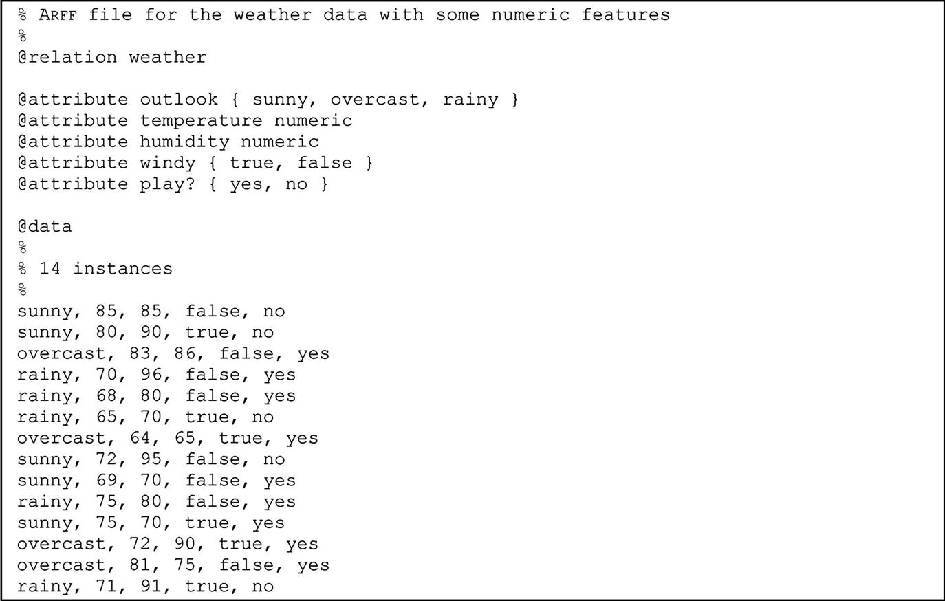
Although the weather problem is to predict the class value play? from the values of the other attributes, the class attribute is not distinguished in any way in the data file. The ARFF format merely gives a dataset; it does not specify which of the attributes is the one that is supposed to be predicted. This means that the same file can be used for investigating how well each attribute can be predicted from the others, or to find association rules, or for clustering.
Following the attribute definitions is an @data line that signals the start of the instances in the dataset. Instances are written one per line, with values for each attribute in turn, separated by commas. If a value is missing it is represented by a single question mark (there are no missing values in this dataset). The attribute specifications in ARFF files allow the dataset to be checked to ensure that it contains legal values for all attributes, and programs that read ARFF files do this checking automatically.
As well as nominal and numeric attributes, exemplified by the weather data, the ARFF format has three further attribute types: string attributes, date attributes, and relation-valued attributes. String attributes have values that are textual. Suppose you have a string attribute that you want to call description. In the block defining the attributes it is specified like this:
@attribute description string
Then, in the instance data, include any character string in quotation marks (to include quotation marks in your string, use the standard convention of preceding each one by a backslash “”). Strings are stored internally in a string table, and represented by their address in that table. Thus two strings that contain the same characters will have the same value.
String attributes can have values that are very long—even a whole document. To be able to use string attributes for text mining, it is necessary to be able to manipulate them. For example, a string attribute might be converted into many numeric attributes, one for each word in the string, whose value is the number of times that word appears. These transformations are described in Section 8.3.
Date attributes are strings with a special format and are introduced like this:
@attribute today date
(for an attribute called today). Weka uses the ISO-8601 combined date and time format yyyy-MM-dd’T’HH:mm:ss with four digits for the year, two each for the month and day, then the letter T followed by the time with two digits for each of hours, minutes, and seconds.1 In the data section of the file dates are specified as the corresponding string representation of the date and time, e.g., 2004-04-03T12:00:00. Although they are specified as strings, dates are converted to numeric form when the input file is read. Dates can also be converted internally to different formats, so you can have absolute timestamps in the data file and use transformations to forms such as time of day or day of the week to detect periodic behavior.
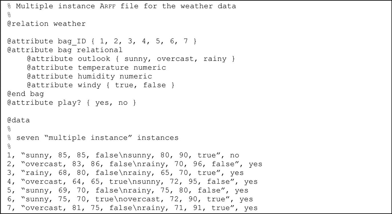
Relation-valued attributes differ from the other types because they allow multi-instance problems to be represented in ARFF format. The value of a relation attribute is a separate set of instances. The attribute is defined with a name and the type relational, followed by a nested attribute block that gives the structure of the referenced instances. For example, a relation-valued attribute called bag whose value is a dataset with the same structure as the weather data but without the play attribute can be specified like this:
@attribute bag relational
@attribute outlook {sunny, overcast, rainy}@attribute temperature numeric
@attribute humidity numeric
@attribute windy {true, false}@end bag
The @end bag indicates the end of the nested attribute block. Fig. 2.3 shows an ARFF file for a multi-instance problem based on the weather data. In this case, each example is made up of an identifier value, two consecutive instances from the original weather data, and a class label. Each value of the attribute is a string that encapsulates two weather instances separated by the “ ” character (which represents an embedded new-line). This might be appropriate for a game that lasts 2 days. A similar dataset might be used for games that last for an indeterminate number of days (e.g., first-class cricket takes 3–5 days). Note, however, that in multi-instance learning the order in which the instances is given is generally considered unimportant. An algorithm might learn that cricket can be played if none of the days is rainy and at least one is sunny, but not that it can only be played in a certain sequence of weather events.
Sparse Data
Sometimes most attributes have a value of 0 for most of the instances. For example, market basket data records purchases made by supermarket customers. No matter how big the shopping expedition, customers never purchase more than a tiny portion of the items a store offers. The market basket data contains the quantity of each item that the customer purchases, and this is 0 for almost all items in stock. The data file can be viewed as a matrix whose rows and columns represent customers and stock items, and the matrix is “sparse”—nearly all its elements are 0. Another example occurs in text mining, where the instances are documents. Here, the columns and rows represent documents and words, and the numbers indicate how many times a particular word appears in a particular document. Most documents have a rather small vocabulary, so most entries are 0.
It can be impractical to represent each element of a sparse matrix explicitly. Instead of representing each value in order, like this:
0, X, 0, 0, 0, 0, Y, 0, 0, 0, “class A”
0, 0, 0, W, 0, 0, 0, 0, 0, 0, “class B”
the nonzero attributes can be explicitly identified by attribute number and their value stated:
{1 X, 6 Y, 10 “class A”}{3 W, 10 “class B”}Each instance is enclosed in braces and contains the index number of each nonzero attribute (indexes start from 0) and its value. Sparse data files have the same @relation and @attribute tags, followed by an @data line, but the data section is different and contains specifications in braces such as those shown previously. Note that the omitted values have a value of 0—they are not “missing” values! If a value is unknown, it must be explicitly represented with a question mark.
Attribute Types
The ARFF format accommodates the two basic data types: nominal and numeric. String attributes and date attributes are effectively nominal and numeric, respectively, although before they are used strings are often converted into a numeric form such as a word vector. Relation-valued attributes contain separate sets of instances that have basic attributes, such as numeric and nominal ones. How the two basic types are interpreted depends on the learning scheme being used. For example, many schemes treat numeric attributes as ordinal scales and only use less-than and greater-than comparisons between the values. However, some treat them as ratio scales and use distance calculations. You need to understand how machine learning schemes work before using them for data mining.
If a learning scheme treats numeric attributes as though they are measured on ratio scales, the question of normalization arises. Attributes are often normalized to lie in a fixed range—usually from zero to one—by dividing all values by the maximum value encountered or by subtracting the minimum value and dividing by the range between the maximum and minimum values. Another normalization technique is to calculate the statistical mean and standard deviation of the attribute values, subtract the mean from each value, and divide the result by the standard deviation. This process is called standardizing a statistical variable and results in a set of values whose mean is zero and standard deviation is one.
Some learning schemes—e.g., instance-based and regression methods—deal only with ratio scales because they calculate the “distance” between two instances based on the values of their attributes. If the actual scale is ordinal, a numeric distance function must be defined. One way of doing this is to use a two-level distance: one if the two values are different and zero if they are the same. Any nominal quantity can be treated as numeric by using this distance function. However, it is rather a crude technique and conceals the true degree of variation between instances. Another possibility is to generate several synthetic binary attributes for each nominal attribute: we return to this in Section 7.3 when we look at the use of trees for numeric prediction.
Sometimes there is a genuine mapping between nominal attributes and numeric scales. For example, postal ZIP codes indicate areas that could be represented by geographical coordinates; the leading digits of telephone numbers may do so too, depending on where you live. The first two digits of a student’s identification number may be the year in which she first enrolled.
It is very common for practical datasets to contain nominal values that are coded as integers. For example, an integer identifier may be used as a code for an attribute such as part number, yet such integers are not intended for use in less-than or greater-than comparisons. If this is the case, it is important to specify that the attribute is nominal rather than numeric.
It is quite possible to treat an ordinal attribute as though it were nominal. Indeed, some machine learning schemes only deal with nominal elements. For example, in the contact lens problem the age attribute is treated as nominal, and the rules generated included these:
If age = young and astigmatic = no
and tear production rate = normal
then recommendation = soft
If age = pre-presbyopic and astigmatic = no
and tear production rate = normal
then recommendation = soft
But in fact age, specified in this way, is really an ordinal attribute for which the following is true:
young < pre-presbyopic < presbyopic.
If it were treated as ordinal, the two rules could be collapsed into one:
If age ≤pre-presbyopic and astigmatic = no
and tear production rate = normal
then recommendation = soft
which is a more compact, and hence more satisfactory, way of saying the same thing.
Missing Values
Most datasets encountered in practice, such as the labor negotiations data in Table 1.6, contain missing values. Missing values are frequently indicated by out-of-range entries; perhaps a negative number (e.g., −1) in a numeric field that is normally only positive, or a 0 in a numeric field that can never normally be 0. For nominal attributes, missing values may be indicated by blanks or dashes. Sometimes different kinds of missing values are distinguished (e.g., unknown vs unrecorded vs irrelevant values) and perhaps represented by different negative integers (−1, −2, etc.).
You have to think carefully about the significance of missing values. They may occur for a number of reasons, such as malfunctioning measurement equipment, changes in experimental design during data collection, and collation of several similar but not identical datasets. Respondents in a survey may refuse to answer certain questions such as age or income. In an archeological study, a specimen such as a skull may be damaged so that some variables cannot be measured. In a biological one, plants or animals may die before all variables have been measured. What do these things mean about the example under consideration? Might the skull damage have some significance in itself, or is it just because of some random event? Does a plant’s early death have some bearing on the case or not?
Most machine learning schemes make the implicit assumption that there is no particular significance in the fact that a certain instance has an attribute value missing: the value is simply not known. However, there may be a good reason why the attribute’s value is unknown—perhaps a decision was taken, on the evidence available, not to perform some particular test—and that might convey some information about the instance other than the fact that the value is simply missing. If this is the case, then it would be more appropriate to record not tested as another possible value for this attribute or perhaps as another attribute in the dataset. As the preceding examples illustrate, only someone familiar with the data can make an informed judgment about whether a particular value being missing has some extra significance or whether it should simply be coded as an ordinary missing value. Of course, if there seem to be several types of missing value, that is prima facie evidence that something is going on that needs to be investigated.
If missing values mean that an operator has decided not to make a particular measurement, that may convey a great deal more than the mere fact that the value is unknown. For example, people analyzing medical databases have noticed that cases may, in some circumstances, be diagnosable simply from the tests that a doctor decides to make regardless of the outcome of the tests. Then a record of which values are “missing” is all that is needed for a complete diagnosis—the actual values can be ignored completely!
Inaccurate Values
It is important to check data mining files carefully for rogue attributes and attribute values. The data used for mining has almost certainly not been gathered expressly for that purpose. When originally collected, many of the fields probably didn’t matter and were left blank or unchecked. Provided it does not affect the original purpose of the data, there is no incentive to correct it. However, when the same database is used for mining, the errors and omissions suddenly start to assume great significance. For example, banks do not really need to know the age of their customers, so their databases may contain many missing or incorrect values. But age may be a very significant feature in mined rules.
Typographic errors in a dataset will obviously lead to incorrect values. Often the value of a nominal attribute is misspelled, creating an extra possible value for that attribute. Or perhaps it is not a misspelling but different names for the same thing, such as Pepsi and Pepsi Cola. Obviously the point of a defined format such as ARFF is to allow data files to be checked for internal consistency. However, errors that occur in the original data file are often preserved through the conversion process into the file that is used for data mining; thus the list of possible values that each attribute takes on should be examined carefully.
Typographical or measurement errors in numeric values generally cause outliers that can be detected by graphing one variable at a time. Erroneous values often deviate significantly from the pattern that is apparent in the remaining values. Sometimes, however, inaccurate values are hard to find, particularly without specialist domain knowledge.
Duplicate data presents another source of error. Most machine learning tools will produce different results if some of the instances in the data files are duplicated, because repetition gives them more influence on the result.
People often make deliberate errors when entering personal data into databases. They might make minor changes in the spelling of their street to try to identify whether the information they have provided ends up being sold to advertising agencies that burden them with junk mail. They might adjust the spelling of their name when applying for insurance if they have had insurance refused in the past. Rigid computerized data entry systems often impose restrictions that require imaginative workarounds. One story tells of a foreigner renting a vehicle in the United States. Being from abroad, he had no ZIP code; yet the computer insisted on one; in desperation the operator suggested that he use the ZIP code of the rental agency. If this is common practice, future data mining projects may notice a cluster of customers who apparently live in the same district as the agency! Similarly, a supermarket checkout operator sometimes uses his own frequent buyer card when the customer does not supply one, either so that the customer can get a discount that would otherwise be unavailable or simply to accumulate credit points in the cashier’s account. Only a deep semantic knowledge of what is going on will be able to explain systematic data errors like these.
Finally, data goes stale. Many items change as circumstances change. For example, items in mailing lists—names, addresses, telephone numbers, and so on—change frequently. You need to consider whether the data you are mining is still current.
Unbalanced Data
In practical applications of classification schemes, it is very often the case that one class is far more prevalent than the others. For example, when predicting the weather in Ireland, it is pretty safe to predict that tomorrow will be rainy rather than sunny. Given a dataset in which these two values form the class attribute, with information relevant to the forecast in the other attributes, excellent accuracy is obtained by predicting rainy regardless of the values of the attributes. In fact, it might be very difficult to come up with a prediction that is numerically more accurate. (A more serious example is the image screening problem of Section 1.3: of the many dark regions in the training data, only a very small fraction are actual oil slicks—fortunately).
Suppose the accuracy if the same class value is predicted for every instance, regardless of the other attributes’ values, is (say) 99%. It’s hard to imagine that a more sophisticated rule could do better. It’s true that there may be better ways of predicting the minority outcome, but these will inevitably make some errors on some cases with the majority outcome. The advantage of better predictions in the 1% of minority-outcome cases will almost certainly be overwhelmed by sacrificing even a tiny bit of accuracy on the 99% cases with the majority outcome.
Always predicting the majority outcome rarely says anything interesting about the data. The problem is that raw accuracy, measured by the proportion of correct predictions, is not necessarily the best criterion of success. In practice, different costs may be associated with the two types of error. If preventative measures are available, the cost of predicting a nuclear disaster (or a death) which turns out not to happen may be serious, but is overwhelmed by the cost of not predicting a nuclear disaster (or a death) if one actually happens. We will consider cost-sensitive evaluation, classification, and learning later in this book.
Getting to Know Your Data
There is no substitute for getting to know your data. Simple tools that show histograms of the distribution of values of nominal attributes, and graphs of the values of numeric attributes (perhaps sorted or simply graphed against instance number), are very helpful. These graphical visualizations of the data make it easy to identify outliers, which may well represent errors in the data file—or arcane conventions for coding unusual situations, such as a missing year as 9999 or a missing weight as −1 kg, that no one has thought to tell you about. Domain experts need to be consulted to explain anomalies, missing values, the significance of integers that represent categories rather than numeric quantities, and so on. Pairwise plots of one attribute against another, or each attribute against the class value, can be extremely revealing.
Data cleaning is a time-consuming and labor-intensive procedure, but one that is absolutely necessary for successful data mining. With a large dataset, people often give up—How can they possibly check it all? Instead, you should sample a few instances and examine them carefully. You’ll be surprised at what you find. Time looking at your data is always well spent.
2.5 Further Reading and Bibliographic Notes
Pyle (1999) provided an extensive guide to data preparation for data mining. There is also a great deal of interest in data warehousing and the problems it entails. Kimball and Ross (2002) is the best introduction to these that we know of. Cabena et al. (1998) estimated that data preparation accounts for 60% of the effort involved in a data mining application, and they write at some length about the problems involved.
The area of inductive logic programming, which deals with finite and infinite relations, was covered by Bergadano and Gunetti (1996). The different “levels of measurement” for attributes were introduced by Stevens (1946) and are well described in the manuals for statistical packages such as SPSS (Nie, Hull, Jenkins, Steinbrenner, & Bent, 1970).
The multi-instance learning setting in its original, quite specific sense, and the drug activity prediction problem that motivated it, was introduced by Dietterich, Lathrop, and Lozano-Perez (1997). The multilabeled instance problem, mentioned near the beginning of Section 2.1, is quite a different setting; Read, Pfahringer, Holmes, and Frank (2009) discussed some approaches for tackling it using standard classification algorithms.