Bias–Variance Decomposition

The effect of combining multiple hypotheses can be viewed through a theoretical device known as the bias–variance decomposition. Suppose we could have an infinite number of independent training sets of the same size and use them to make an infinite number of classifiers. A test instance is processed by all classifiers, and a single answer is determined by majority vote. In this idealized situation, errors will still occur because no learning scheme is perfect: the error rate will depend on how well the machine learning method matches the problem at hand, and there is also the effect of noise in the data, which cannot possibly be learned. Suppose the expected error rate were evaluated by averaging the error of the combined classifier over an infinite number of independently chosen test examples. The error rate for a particular learning algorithm is called its bias for the learning problem and measures how well the learning method matches the problem. (We include the “noise” component in the bias term because it is generally unknown in practice anyway.) This technical definition is a way of quantifying the vaguer notion of bias that was introduced in Section 1.5: it measures the “persistent” error of a learning algorithm that can’t be eliminated even by taking an infinite number of training sets into account. Of course, it cannot be calculated exactly in practical situations; it can only be approximated.

A second source of error in a learned model, in a practical situation, stems from the particular training set used, which is inevitably finite and therefore not fully representative of the actual population of instances. The expected value of this component of the error, over all possible training sets of the given size and all possible test sets, is called the variance of the learning method for that problem. The total expected error of a classifier is made up of the sum of bias and variance: this is the bias–variance decomposition.

Note that we are glossing over the details here. The bias–variance decomposition was introduced in the context of numeric prediction based on squared error, where there is a widely accepted way of performing it. However, the situation is not so clear for classification, and several competing decompositions have been proposed. Regardless of the specific decomposition used to analyze the error, combining multiple classifiers generally decreases the expected error by reducing the variance component. The more classifiers that are included, the greater the reduction in variance. Of course, a difficulty arises when putting this voting scheme into practice: usually there is only one training set, and obtaining more data is either impossible or expensive.

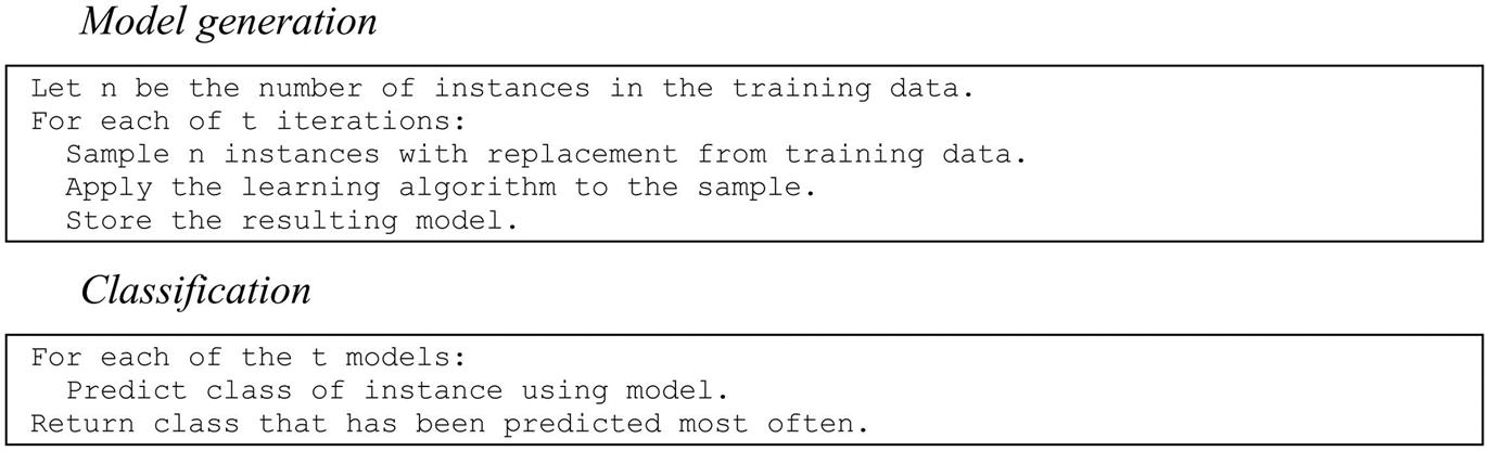
Bagging attempts to neutralize the instability of learning methods by simulating the process described previously using a given training set. Instead of sampling a fresh, independent training dataset each time, the original training data is altered by deleting some instances and replicating others. Instances are randomly sampled, with replacement, from the original dataset to create a new one of the same size. This sampling procedure inevitably replicates some of the instances and deletes others. If this idea strikes a chord, it is because we encountered it in Chapter 5, Credibility: evaluating what’s been learned, when explaining the bootstrap method for estimating the generalization error of a learning method (Section 5.4): indeed, the term bagging stands for bootstrap aggregating. Bagging applies the learning scheme—e.g., a decision tree inducer—to each one of these artificially derived datasets, and the classifiers generated from them vote for the class to be predicted. The algorithm is summarized in Fig. 12.1.

The difference between bagging and the idealized procedure described above is the way in which the training datasets are derived. Instead of obtaining independent datasets from the domain, bagging just resamples the original training data. The datasets generated by resampling are different from one another but are certainly not independent because they are all based on one dataset. However, it turns out that bagging produces a combined model that often performs significantly better than the single model built from the original training data, and is never substantially worse.

Bagging can also be applied to learning schemes for numeric prediction—e.g., model trees. The only difference is that, instead of voting on the outcome, the individual predictions, being real numbers, are averaged. The bias–variance decomposition is applied to numeric prediction by decomposing the expected value of the mean-squared error of the predictions on fresh data. Bias is defined as the mean-squared error expected when averaging over models built from all possible training datasets of the same size, and variance is the component of the expected error of a single model that is due to the particular training data it was built from. It can be shown theoretically that averaging over infinitely many models built from independent training sets always reduces the expected value of the mean-squared error. (As we mentioned earlier, the analogous result is not true for classification.)

Bagging With Costs

Bagging helps most if the underlying learning scheme is unstable in that small changes in the input data can lead to quite different classifiers. Indeed results can be improved by increasing the diversity in the ensemble of classifiers by making the learning scheme as unstable as possible, while maintaining some level of accuracy. For example, when bagging decision trees, which are already unstable, better performance is often achieved by switching pruning off, which makes them even more unstable. Another improvement can be obtained by changing the way that predictions are combined for classification. As originally formulated, bagging uses voting. But when the models can output probability estimates and not just plain classifications, it makes intuitive sense to average these probabilities instead. Not only does this often improve classification slightly, but the bagged classifier also generates probability estimates—ones that are often more accurate than those produced by the individual models. Implementations of bagging commonly use this method of combining predictions.

In Section 5.8 we showed how to make a classifier cost sensitive by minimizing the expected cost of predictions. Accurate probability estimates are necessary because they are used to obtain the expected cost of each prediction. Bagging is a prime candidate for cost-sensitive classification because it produces very accurate probability estimates from decision trees and other powerful, yet unstable, classifiers. However, a disadvantage is that bagged classifiers are hard to analyze.

A method called MetaCost combines the predictive benefits of bagging with a comprehensible model for cost-sensitive prediction. It builds an ensemble classifier using bagging and deploys it to relabel the training data by giving every training instance the prediction that minimizes the expected cost, based on the probability estimates obtained from bagging. MetaCost then discards the original class labels and learns a single new classifier—e.g., a single pruned decision tree—from the relabeled data. This new model automatically takes costs into account because they have been built into the class labels! The result is a single cost-sensitive classifier that can be analyzed to see how predictions are made.

In addition to the cost-sensitive classification technique just mentioned, Section 5.8 also described a cost-sensitive learning method that learns a cost-sensitive classifier by changing the proportion of each class in the training data to reflect the cost matrix. MetaCost seems to produce more accurate results than this method, but it requires more computation. If there is no need for a comprehensible model, MetaCost’s postprocessing step is superfluous: it is better to use the bagged classifier directly in conjunction with the minimum expected cost method.

Randomization Versus Bagging

Randomization demands more work than bagging because the learning algorithm must be modified, but it can profitably be applied to a greater variety of learners. We noted earlier that bagging fails with stable learning algorithms whose output is insensitive to small changes in the input. For example, it is pointless to bag nearest-neighbor classifiers because their output changes very little if the training data is perturbed by sampling. But randomization can be applied even to stable learners: the trick is to randomize in a way that makes the classifiers diverse without sacrificing too much performance. A nearest-neighbor classifier’s predictions depend on the distances between instances, which in turn depend heavily on which attributes are used to compute them, so nearest-neighbor classifiers can be randomized by using different, randomly chosen subsets of attributes. In fact, this approach is called the random subspaces method for constructing an ensemble of classifiers and was proposed as a method for learning a random forest. As with bagging, it does not require any modification to the learning algorithm. Of course, random subspaces can be used in conjunction with bagging in order to introduce randomness to the learning process in terms of both instances and attributes.

Returning to plain bagging, the idea is to exploit instability in the learning algorithm in order to create diversity amongst the ensemble members—but the degree of diversity achieved is less than that of other ensemble learning methods such as random forests, because of randomization built in to the learning algorithm, or boosting (discussed in Section 12.4). This is because bootstrap sampling creates training datasets whose distribution resembles that of the original data. Consequently, the classifiers learned by bagging are individually quite accurate, but their low diversity can detract from the overall accuracy of the ensemble. Introducing randomness in the learning algorithm increases diversity but sacrifices accuracy of the individual classifiers. If it were possible for ensemble members to be both diverse and individually accurate, smaller ensembles could be used. Of course, this would have computational benefits.

Rotation Forests

An ensemble learning method called rotation forests has the specific goal of creating diverse yet accurate classifiers. It combines the random subspace and bagging approaches with principal component feature generation to construct an ensemble of decision trees. In each iteration, the input attributes are randomly divided into k disjoint subsets. Principal component analysis is applied to each subset in turn in order to create linear combinations of the attributes in the subset that are rotations of the original axes. The k sets of principal components are used to compute values for the derived attributes; these comprise the input to the tree learner at each iteration. Because all the components obtained on each subset are retained, there are as many derived attributes as there are original ones. To discourage the generation of identical coefficients if the same feature subset is chosen in different iterations, principal component analysis is applied to training instances from a randomly chosen subset of the class values (however, the values of the derived attributes that are input to the tree learner are computed from all the instances in the training data). To further increase diversity, a bootstrap sample of the data can be created in each iteration before the principal component transformations are applied.

Experiments indicate that rotation forests can give similar performance to random forests, with far fewer trees. An analysis of diversity (measured by the Kappa statistic, introduced in Section 5.8 to measure agreement between classifiers) versus error for pairs of ensemble members shows a minimal increase in diversity and reduction in error for rotation forests when compared to bagging. However, this appears to translate into significantly better performance for the ensemble as a whole.

AdaBoost

There are many variants on the idea of boosting. We describe a widely used method called AdaBoost.M1 that is designed specifically for classification. Like bagging, it can be applied to any classification learning algorithm. To simplify matters we assume that the learning algorithm can handle weighted instances, where the weight of an instance is a positive number. (We revisit this assumption later.) The presence of instance weights changes the way in which a classifier’s error is calculated: it is the sum of the weights of the misclassified instances divided by the total weight of all instances, instead of the fraction of instances that are misclassified. By weighting instances, the learning algorithm can be forced to concentrate on a particular set of instances, namely, those with high weight. Such instances become particularly important because there is a greater incentive to classify them correctly. The C4.5 algorithm, described in Section 6.1, is an example of a learning method that can accommodate weighted instances without modification because it already uses the notion of fractional instances to handle missing values.

The boosting algorithm, summarized in Fig. 12.2, begins by assigning equal weight to all instances in the training data. It then calls the learning algorithm to form a classifier for this data and reweights each instance according to the classifier’s output. The weight of correctly classified instances is decreased, and that of misclassified ones is increased. This produces a set of “easy” instances with low weight and a set of “hard” ones with high weight. In the next iteration—and all subsequent ones—a classifier is built for the reweighted data, which consequently focuses on classifying the hard instances correctly. Then the instances’ weights are increased or decreased according to the output of this new classifier. As a result, some hard instances might become even harder and easier ones even easier; on the other hand, other hard instances might become easier, and easier ones harder—all possibilities can occur in practice. After each iteration, the weights reflect how often the instances have been misclassified by the classifiers produced so far. By maintaining a measure of “hardness” with each instance, this procedure provides an elegant way of generating a series of experts that complement one another.

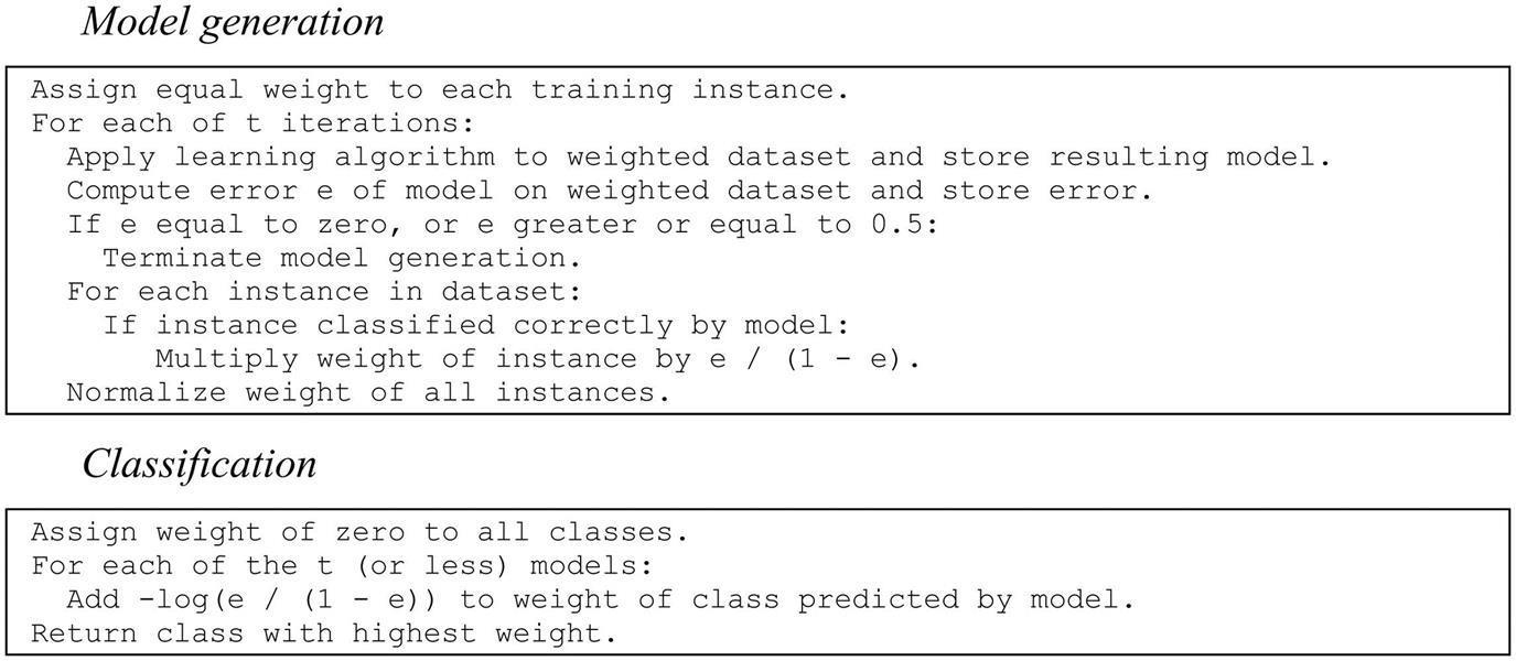
How much should the weights be altered after each iteration? The answer depends on the current classifier’s overall error. More specifically, if e denotes the classifier’s error on the weighted data (a fraction between 0 and 1), then weights are updated by

$\mathrm{Weight}\leftarrow \mathrm{Weight}\times e/(1-e)$

for correctly classified instances, and the weights remain unchanged for misclassified ones. Of course, this does not increase the weight of misclassified instances as claimed earlier. However, after all weights have been updated they are renormalized so that their sum remains the same as it was before. Each instance’s weight is divided by the sum of the new weights and multiplied by the sum of the old ones. This automatically increases the weight of each misclassified instance and reduces that of each correctly classified one.

Whenever the error on the weighted training data exceeds or equals 0.5, the boosting procedure deletes the current classifier and does not perform any more iterations. The same thing happens when the error is 0, because then all instance weights become 0.

We have explained how the boosting method generates a series of classifiers. To form a prediction, their output is combined using a weighted vote. To determine the weights, note that a classifier that performs well on the weighted training data from which it was built (e close to 0) should receive a high weight, and a classifier that performs badly (e close to 0.5) should receive a low one. The AdaBoost.M1 algorithm uses

$\mathrm{Weight}=-\log \frac{e}{1-e},$

which is a positive number between 0 and infinity. Incidentally, this formula explains why classifiers that perform perfectly on the training data must be deleted, because when e is 0 the weight is undefined. To make a prediction, the weights of all classifiers that vote for a particular class are summed, and the class with the greatest total is chosen.

We began by assuming that the learning algorithm can cope with weighted instances. Any algorithm can be adapted to deal with weighted instances; we explained how at the end of Section 7.3 under Locally weighted linear regression. Instead of changing the learning algorithm, it is possible to generate an unweighted dataset from the weighted data by resampling—the same technique that bagging uses. Whereas for bagging each instance is chosen with equal probability, for boosting instances are chosen with probability proportional to their weight. As a result, instances with high weight are replicated frequently, and ones with low weight may never be selected. Once the new dataset becomes as large as the original one, it is fed into the learning scheme instead of the weighted data. It’s as simple as that.

A disadvantage of this procedure is that some instances with low weight do not make it into the resampled dataset, so information is lost before the learning scheme is applied. However, this can be turned into an advantage. If the learning scheme produces a classifier whose error exceeds 0.5, boosting must terminate if the weighted data is used directly, whereas with resampling it might be possible to produce a classifier with error below 0.5 by discarding the resampled dataset and generating a new one from a different random seed. Sometimes more boosting iterations can be performed by resampling than when using the original weighted version of the algorithm.

The Power of Boosting

The idea of boosting originated in a branch of machine learning research known as computational learning theory. Theoreticians are interested in boosting because it is possible to derive performance guarantees. For example, it can be shown that the error of the combined classifier on the training data approaches zero very quickly as more iterations are performed (exponentially quickly in the number of iterations). Unfortunately, as explained in Section 5.1, guarantees for the training error are not very interesting because they do not necessarily indicate good performance on fresh data. However, it can be shown theoretically that boosting only fails on fresh data if the individual classifiers are too “complex” for the amount of training data present or their training errors become too large too quickly. As usual, the problem lies in finding the right balance between the individual models’ complexity and their fit to the data.

If boosting does succeed in reducing the error on fresh test data, it often does so in a spectacular way. One very surprising finding is that performing more boosting iterations can reduce the error on new data long after the classification error of the combined classifier on the training data has dropped to zero. Researchers were puzzled by this result because it seems to contradict Occam’s razor, which declares that, of two hypotheses that explain the empirical evidence equally well the simpler one is to be preferred. Performing more boosting iterations without reducing training error does not explain the training data any better, and it certainly adds complexity to the combined classifier. The contradiction can be resolved by considering the classifier’s confidence in its predictions. More specifically, we measure confidence by the difference between the estimated confidence for the true class and that of the most likely predicted class other than the true class—a quantity known as the margin. The larger the margin, the more confident the classifier is in predicting the true class. It turns out that boosting can increase the margin long after the training error has dropped to zero. The effect can be visualized by plotting the cumulative distribution of the margin values of all the training instances for different numbers of boosting iterations, giving a graph known as the margin curve. Hence, if the explanation of empirical evidence takes the margin into account, Occam’s razor remains as sharp as ever.

The beautiful thing about boosting is that a powerful combined classifier can be built from very simple ones as long as they achieve less than 50% error on the reweighted data. Usually, this is easy—certainly for learning problems with two classes! Simple learning schemes are called weak learners, and boosting converts weak learners into strong ones. For example, good results for two-class problems can be obtained by boosting extremely simple decision trees that have only one level—called decision stumps. Another possibility is to apply boosting to an algorithm that learns a single conjunctive rule—such as a single path in a decision tree—and classifies instances based on whether or not the rule covers them. Of course, multiclass datasets make it more difficult to achieve error rates below 0.5. Decision trees can still be boosted, but they usually need to be more complex than decision stumps. More sophisticated algorithms have been developed that allow very simple models to be boosted successfully in multiclass situations.

Boosting often produces classifiers that are significantly more accurate on fresh data than ones generated by bagging. However, unlike bagging, boosting sometimes fails in practical situations: it can generate a classifier that is significantly less accurate than a single classifier built from the same data. This indicates that the combined classifier overfits the data.

Numeric Prediction

Here is a well-known forward stagewise additive modeling method for numeric prediction. First, build a standard regression model, e.g., a regression tree. The errors it exhibits on the training data—the differences between predicted and observed values—are called residuals. Then correct for these errors by learning a second model—perhaps another regression tree—that tries to predict the observed residuals. To do this, simply replace the original class values by their residuals before learning the second model. Adding the predictions made by the second model to those of the first one automatically yields lower error on the training data. Usually some residuals still remain, because the second model is not a perfect one, so we continue with a third model that learns to predict the residuals of the residuals, and so on. The procedure is reminiscent of the use of rules with exceptions for classification that we met in Section 3.4.

If the individual models minimize the squared error of the predictions, as linear regression models do, this algorithm minimizes the squared error of the ensemble as a whole. In practice it also works well when the base learner uses a heuristic approximation instead, such as the regression and model tree learners described in Section 7.3. In fact, there is no point in using standard linear regression as the base learner for additive regression, because the sum of linear regression models is again a linear regression model and the regression algorithm itself minimizes the squared error. However, it is a different story if the base learner is a regression model based on a single attribute, the one that minimizes the squared error. Statisticians call this simple linear regression, in contrast to the standard multiattribute method, properly called multiple linear regression. In fact, using additive regression in conjunction with simple linear regression and iterating until the squared error of the ensemble decreases no further yields an additive model identical to the least-squares multiple linear regression function.

Forward stagewise additive regression is prone to overfitting because each model added fits the training data closer and closer. To decide when to stop, use cross-validation. For example, perform a cross-validation for every number of iterations up to a user-specified maximum and choose the one that minimizes the cross-validated estimate of squared error. This is a good stopping criterion because cross-validation yields a fairly reliable estimate of the error on future data. Incidentally, using this method in conjunction with simple linear regression as the base learner effectively combines multiple linear regression with built-in attribute selection, because the next most important attribute’s contribution is only included if it decreases the cross-validated error.

For implementation convenience, forward stagewise additive regression usually begins with a level-0 model that simply predicts the mean of the class on the training data so that every subsequent model fits residuals. This suggests another possibility for preventing overfitting: instead of subtracting a model’s entire prediction to generate target values for the next model, shrink the predictions by multiplying them by a user-specified constant factor between 0 and 1 before subtracting. This reduces the model’s fit to the residuals, and consequently reduces the chance of overfitting. Of course, it may increase the number of iterations needed to arrive at a good additive model. Reducing the multiplier effectively damps down the learning process, increasing the chance of stopping at just the right moment—but also increasing run time.

Additive Logistic Regression

Additive regression can also be applied to classification just as linear regression can. But we know from Section 4.6 that logistic regression is more suitable than linear regression for classification. It turns out that a similar adaptation can be made to additive models by modifying the forward stagewise modeling method to perform additive logistic regression. Use the logit transform to translate the probability estimation problem into a regression problem, as we did in Section 4.6, and solve the regression task using an ensemble of models—e.g., regression trees—just as for additive regression. At each stage, add the model that maximizes the probability of the data given the ensemble classifier.

Suppose f_j is the jth regression model in the ensemble and f_j(a) is its prediction for instance a. Assuming a two-class problem, use the additive model $\sum f_j(\mathbf{a})$ to obtain a probability estimate for the first class:

$p(1|\mathbf{a})=\frac{1}{1+e^{-\sum f_j(\mathbf{a})}}.$

This closely resembles the expression used in Section 4.6, except that here it is abbreviated by using vector notation for the instance a and the original weighted sum of attributes values is replaced by a sum of arbitrarily complex regression models f.

Fig. 12.3 shows the two-class version of the so-called LogitBoost algorithm, which performs additive logistic regression and generates the individual models f_j. Here, y_i is 1 for an instance in the first class and 0 for an instance in the second. In each iteration this algorithm fits a regression model f_j to a weighted version of the original dataset based on dummy class values z_i and weights w_i. We assume that $p(1|\mathbf{a})$ is computed using the f_j that were built in previous iterations.

The derivation of this algorithm is beyond the scope of this book, but it can be shown that the algorithm maximizes the probability of the data with respect to the ensemble if each model f_j is determined by minimizing the squared error on the corresponding regression problem. In fact, if multiple linear regression is used to form the f_j, the algorithm converges to the maximum likelihood linear-logistic regression model: it is an incarnation of the iteratively reweighted least-squares method mentioned in Section 4.6.

Superficially, LogitBoost looks quite different to AdaBoost, but the predictors they produce differ mainly in that the former optimizes the likelihood directly whereas the latter optimizes an exponential loss function that can be regarded as an approximation to it. From a practical perspective, the difference is that LogitBoost uses a regression scheme as the base learner whereas AdaBoost works with classification algorithms.

We have only shown the two-class version of LogitBoost, but the algorithm can be generalized to multiclass problems. As with additive regression, the danger of overfitting can be reduced by shrinking the predictions of the individual f_j by a predetermined multiplier and using cross-validation to determine an appropriate number of iterations.

Option Trees

Another approach is to derive a single structure that can represent an ensemble of classifiers compactly. This can be done if the ensemble consists of decision trees; the result is called an option tree. Option trees differ from decision trees in that they contain two types of node: decision nodes and option nodes. Fig. 12.4 shows a simple example for the weather data, with only one option node. To classify an instance, filter it down through the tree. At a decision node take just one of the branches, as usual, but at an option node take all the branches. This means that the instance ends up in more than one leaf, and the classifications obtained from those leaves must somehow be combined into an overall classification. This can be done simply by voting, taking the majority vote at an option node to be the prediction of the node. In that case it makes little sense to have option nodes with only two options (as in Fig. 12.4) because there will only be a majority if both branches agree. Another possibility is to average the probability estimates obtained from the different paths, using either an unweighted average or a more sophisticated Bayesian approach.

Option trees can be generated by modifying an existing decision tree learner to create an option node if there are several splits that look similarly useful according to their information gain. All choices within a certain user-specified tolerance of the best one can be made into options. During pruning, the error of an option node is the average error of its options.

Another possibility is to grow an option tree by incrementally adding nodes to it. This is commonly done using a boosting algorithm, and the resulting trees are usually called alternating decision trees instead of option trees. In this context the decision nodes are called splitter nodes and the option nodes are called prediction nodes. Prediction nodes are leaves if no splitter nodes have been added to them yet. The standard alternating decision tree applies to two-class problems, and with each prediction node is associated a positive or negative numeric value. To obtain a prediction for an instance, filter down all applicable branches and sum up the values from any prediction nodes that are encountered; predict one class or the other depending on whether the sum is positive or negative.

A simple example tree for the weather data is shown in Fig. 12.5, where a positive value corresponds to class play=no and a negative one to play=yes. To classify an instance with outlook=sunny, temperature=hot, humidity=normal, and windy=false, filter it down to the corresponding leaves, obtaining values −0.255, 0.213, −0.430, and −0.331. The sum of these values is negative; hence predict play=yes. Alternating decision trees always have a prediction node at the root, as in this example.

The alternating tree is grown using a boosting algorithm—e.g., a boosting algorithm that employs a base learner for numeric prediction, such as the LogitBoost method described previously. Assume that the base learner produces a single conjunctive rule in each boosting iteration. Then an alternating decision tree can be generated by simply adding each rule into the tree. The numeric scores associated with the prediction nodes are obtained from the consequents of the rules. However, the resulting tree will grow large very quickly because the rules from different boosting iterations are likely to be different. Hence, learning algorithms for alternating decision trees consider only those rules that extend one of the existing paths in the tree by adding a splitter node and two corresponding prediction nodes (assuming binary splits). In the standard version of the algorithm, every possible location in the tree is considered for addition, and a node is added according to a performance measure that depends on the particular boosting algorithm employed. However, heuristics can be used instead of an exhaustive search to speed up the learning process.

Logistic Model Trees

Option trees and alternating trees yield very good classification performance based on a single structure, but they may still be difficult to interpret when there are many options nodes because it becomes difficult to see how a particular prediction is derived. However, it turns out that boosting can also be used to build very effective decision trees that do not include any options at all. For example, the LogitBoost algorithm has been used to induce trees with linear-logistic regression models at the leaves. These are called logistic model trees and are interpreted in the same way as the model trees for regression described in Section 7.3.

LogitBoost performs additive logistic regression. Suppose that each iteration of the boosting algorithm fits a simple regression function by going through all the attributes, finding the simple regression function with the smallest error, and adding it into the additive model. If the LogitBoost algorithm is run until convergence, the result is a maximum likelihood multiple-logistic regression model. However, for optimum performance on future data it is usually unnecessary to wait for convergence—and to do so is often detrimental. An appropriate number of boosting iterations can be determined by estimating the expected performance for a given number of iterations using cross-validation and stopping the process when performance ceases to increase.

A simple extension of this algorithm leads to logistic model trees. The boosting process terminates when there is no further structure in the data that can be modeled using a linear-logistic regression function. However, there may still be structure that linear models can fit if attention is restricted to subsets of the data, obtained, e.g., by splitting the data using a standard decision tree criterion such as information gain. Thus, once no further improvement can be obtained by adding more simple linear models, the data is split and boosting resumed separately in each subset. This process takes the logistic model generated so far and refines it separately for the data in each subset. Again, cross-validation is run in each subset to determine an appropriate number of iterations to perform in that subset.

The process is applied recursively until the subsets become too small. The resulting tree will surely overfit the training data, and one of the standard methods of decision tree learning can be used to prune it. Experiments indicate that the pruning operation is very important. Using the cost-complexity pruning method discussed in Section 6.1, which chooses the right tree size using cross-validation, the algorithm produces small but very accurate trees with linear-logistic models at the leaves.