This is ordinary linear regression!

Although x_i is a scalar here, the method generalizes to a vector x_i. Categorical variables can be encoded into a subset of the dimensions of x using the so-called “one-hot” method, placing a 1 in the dimension corresponding to the category label and 0s in all other dimensions allocated to the variable. If all input variables are categorical, this corresponds to the classic analysis of variance (ANOVA) method.

Using Priors on Parameters

Placing a Gaussian prior on the parameters w leads to the method of ridge regression (Section 7.2)— also called “weight decay.” Consider a regression that uses a D-dimensional vector x to make predictions. The regression’s bias term can be represented by defining the first dimension of x as the constant 1 for every example. Defining $\left[{\theta }_1\dots {\theta }_D\right]={\mathbf{w}}^T$ and using the usual $N(x;\mu ,\sigma )$ notation for scalar Gaussians, the underlying probability model is

${\prod }_{i=1}^{N}p(y_i|x_i;\theta )p(\theta ;\tau )=\left[{\prod }_{i=1}^{N}N(y_i;{\mathbf{w}}^T{x}_i,{\sigma }^2)\right]\left[{\prod }_{d=1}^{D}N(w_d;0,{\tau }^2)\right],$

where τ is the hyperparameter specifying the prior. Setting $\lambda \equiv {\sigma }^2/{\tau }^2$, it is possible to show that maximum a posteriori parameter estimation based on the log conditional likelihood is equivalent to minimizing the squared error loss function

$F(\mathbf{w})=\sum _{i=1}^N{\{y_i-{\mathbf{w}}^T{x}_i\}}^2+\lambda {\mathbf{w}}^T\mathbf{w},$ (9.4)

(9.4)

which includes an L₂-based regularization term given by $R_{L_2}(\mathbf{w})={\mathbf{w}}^T\mathbf{w}=||\mathbf{w}|{|}_2^2$. (“Regularization” is another term for overfitting avoidance.)

Using a Laplace prior for the distribution over weights and taking the log of the likelihood function yields an L₁-based regularization term $R_{L_1}(\mathbf{w})=||\mathbf{w}|{|}_1$. To see why, note that the Laplace distribution has the form

$P(w;\mu ,b)=L(w;\mu ,b)=\frac{1}{2b}\exp \left(-\frac{|w-\mu |}{b}\right),$

where $\mu$ and b are parameters. Modeling the prior probability for each weight by a Laplace distribution with ${\mu }_j=0$ yields

$-\log \left[\prod _{d=1}^{D}L(w_d;0,b)\right]=\log (2b)+\frac{1}{b}\sum _{d=1}^D|w_d|\propto ||\mathbf{w}|{|}_1.$

Since the Laplace distribution places more probability at zero than the Gaussian distribution does, it can provide both regularization and variable selection in regression problems. This technique has been popularized as a regression approach known as the LASSO, “Least Absolute Shrinkage and Selection Operator.”

An alternative approach known as the “elastic net” combines L₁ and L₂ regularization techniques using

${\lambda }_1{R}_{L_1}(\mathbf{\theta })+{\lambda }_2{R}_{L_2}(\mathbf{\theta })={\lambda }_1||\mathbf{w}|{|}_1+{\lambda }_2||\mathbf{w}|{|}_2^2.$

This corresponds to a prior distribution that consist of the product of a Gaussian and a Laplacian distribution. The result leads to convex optimization problems—i.e., problems where any local minimum must be a global minimum—if the loss is convex, which applies to models like logistic or linear regression.

Matrix vector formulations of linear and polynomial regression

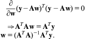
This section formulates linear regression using matrix operations. Observe that the loss in (9.4)—without the penalty term—can be written

$\begin{array}{l}\sum _{i=1}^N{\{y_i-({\theta }_0+{\theta }_1{x}_{1i}+{\theta }_2{x}_{2i}+\dots +{\theta }_D{x}_{Di})\}}^2\hfill \\ ={\left(\left[\begin{array}{c}{y}_1\\ ⋮\\ y_N\end{array}\right]-\left[\begin{array}{ccccc}1& x_{11}& x_{21}& & x_{D1}\\ ⋮& ⋮& ⋮& \cdots & ⋮\\ 1& x_{1N}& x_{2N}& & x_{DN}\end{array}\right]\left[\begin{array}{c}{\theta }_0\\ ⋮\\ {\theta }_D\end{array}\right]\right)}^T\left(\left[\begin{array}{c}{y}_1\\ ⋮\\ y_N\end{array}\right]-\left[\begin{array}{ccccc}1& x_{11}& x_{21}& & x_{D1}\\ ⋮& ⋮& ⋮& \cdots & ⋮\\ 1& x_{1N}& x_{2N}& & x_{DN}\end{array}\right]\left[\begin{array}{c}{\theta }_0\\ ⋮\\ {\theta }_D\end{array}\right]\right)\hfill \\ ={(\mathbf{y}-\mathbf{A}\mathbf{w})}^T(\mathbf{y}-\mathbf{A}\mathbf{w}).\hfill \end{array}$

where the vector y is just the individual y_i’s stacked up, and w is the vector of parameters (or weights) for the model. Taking the partial derivative with respect to w and setting the result to zero yields a closed form expression for the parameters:

$\begin{array}{l}\frac{\partial }{\partial \mathbf{w}}{(\mathbf{y}-\mathbf{A}\mathbf{w})}^T(\mathbf{y}-\mathbf{A}\mathbf{w})=0\hfill \\ \Rightarrow {\mathbf{A}}^T\mathbf{A}\mathbf{w}={\mathbf{A}}^T\mathbf{y}\hfill \\ \mathbf{w}={({\mathbf{A}}^T\mathbf{A})}^{-1}{\mathbf{A}}^T\mathbf{y}.\hfill \end{array}$ (9.5)

(9.5)

These are famous equations. ${\mathbf{A}}^T\mathbf{A}\mathbf{w}={\mathbf{A}}^T\mathbf{y}$ is known as the normal equations, and the quantity ${\mathbf{A}}^{+}={({\mathbf{A}}^T\mathbf{A})}^{-1}{\mathbf{A}}^T$ is known as the pseudoinverse. Note that ${\mathbf{A}}^T\mathbf{A}$ is not always invertible, but this problem can be addressed using regularization.

For ridge regression, a prior is added to make the objective function

$F(\mathbf{w})={(\mathbf{y}-\mathbf{A}\mathbf{w})}^T(\mathbf{y}-\mathbf{A}\mathbf{w})+\lambda {\mathbf{w}}^T\mathbf{w},$ (9.6)

(9.6)

for a suitably defined matrix A with vectors x_i in the rows, and $\lambda$ as defined above. Again, setting the partial derivative of F(w) to zero yields a closed form solution:

$\begin{array}{l}\frac{\partial }{\partial \mathbf{w}}F(\mathbf{w})=0\hfill \\ \Rightarrow {\mathbf{A}}^T\mathbf{A}\mathbf{w}+\lambda \mathbf{w}={\mathbf{A}}^T\mathbf{y}\hfill \\ \mathbf{w}={({\mathbf{A}}^T\mathbf{A}+\lambda \mathbf{I})}^{-1}{\mathbf{A}}^T\mathbf{y}.\hfill \end{array}$

This modification to the pseudoinverse equation allows solutions to be found that would otherwise not exist, often using a very small $\lambda$. It is often presented as a regularization method that avoids numerical instability, but the analysis in terms of a prior on parameters gives more insight. For example, it may be appropriate to use Gaussian priors of different strengths for different terms. In fact, it is common practice to impose no penalty at all on the bias weight. This could be implemented by replacing the $\lambda {\mathbf{w}}^T\mathbf{w}$ term in (9.6) by ${\mathbf{w}}^T\mathbf{D}\mathbf{w}$, where D is a diagonal matrix containing the λ_i’s to be used for each weight, transforming the solution into $\mathbf{w}={({\mathbf{A}}^T\mathbf{A}+\mathbf{D})}^{-1}{\mathbf{A}}^T\mathbf{y}$. While the above expression for the partial derivative is fairly simple, care must still be taken during implementation to avoid numerically instable results.

The linear regression model can be transformed into a nonlinear polynomial model. Although the polynomial regression model yields nonlinear predictions, the estimation problem is linear in the parameters. To see this, express the problem in matrix form, using a suitably defined matrix A to encode the polynomial’s higher order terms and a vector c to encode the coefficients, including those used for the higher order terms:

$\begin{array}{l}\sum _{i=1}^N{\{y_i-({\theta }_0+{\theta }_1{x}_i+{\theta }_2{x}_i^2+\cdots +{\theta }_K{x}_i^K)\}}^2\hfill \\ ={\left(\left[\begin{array}{c}{y}_1\\ ⋮\\ y_N\end{array}\right]-\left[\begin{array}{ccccc}1& x_1& x_1^2& & x_1^K\\ ⋮& ⋮& ⋮& \cdots & ⋮\\ 1& x_N& x_N^2& & x_N^K\end{array}\right]\left[\begin{array}{c}{\theta }_0\\ ⋮\\ {\theta }_K\end{array}\right]\right)}^{\mathbf{T}}\left(\left[\begin{array}{c}{y}_1\\ ⋮\\ y_N\end{array}\right]-\left[\begin{array}{ccccc}1& x_1& x_1^2& & x_1^K\\ ⋮& ⋮& ⋮& \cdots & ⋮\\ 1& x_N& x_N^2& & x_N^K\end{array}\right]\left[\begin{array}{c}{\theta }_0\\ ⋮\\ {\theta }_K\end{array}\right]\right)\hfill \\ ={(\mathbf{y}-\mathbf{A}\mathbf{c})}^T(\mathbf{y}-\mathbf{A}\mathbf{c}).\hfill \end{array}$

Eq. (9.5) can be used to solve for the parameters in closed form.

This trick of transforming a linear prediction method into a nonlinear one while keeping the underlying estimation problem linear can be generalized. The general approach goes by the name of basis function expansion. For polynomial regression, the polynomial basis given by the rows of the matrix A (the powers of x) is used. However, any nonlinear function of the inputs $\mathbf{\varphi }(\mathbf{x})$ could be used to define models of the form

$p(y|\mathbf{x})=N(y;{\mathbf{w}}^T\mathbf{\varphi }(\mathbf{x}),{\sigma }^2),$

which also give closed form solutions for a linear parameter estimation problem. We will return to this when discussing kernelizing probabilistic models below.

Multiclass Logistic Regression

Binary logistic regression was introduced in Section 4.6. Consider now a multiclass classification problem where class values are encoded as instances of the random variable $y\in \{1,\dots ,N\}$, and, as before, feature vectors are instances of a variable x. Assume there is no significance to the order of the classes.

A simple linear probabilistic classifier can be created using this parametric form:

$p(y|\mathbf{x})=\frac{\exp \left({\sum }_{k=1}^K{w}_k{f}_k(y,\mathbf{x})\right)}{\sum _y\exp \left({\sum }_{k=1}^K{w}_k{f}_k(y,\mathbf{x})\right)}=\frac{1}{Z(\mathbf{x})}\exp \left(\sum _{k=1}^K{w}_k{f}_k(y,\mathbf{x})\right),$ (9.7)

(9.7)

which employs K feature functions f_k(y,x) and K weights, w_k as the parameters of the model. This is one way of formulating multinomial logistic regression. The feature functions could encode complex features extracted from the input vector x. To perform learning using maximum conditional likelihood and observations that are instances of y and x, $\{{\tilde{y}}_1,\dots ,{\tilde{y}}_N,{\tilde{\mathbf{x}}}_1,\dots ,{\tilde{\mathbf{x}}}_N\}$, write the objective function as

$L_{y|x}=\log \prod _{i=1}^{N}p({\tilde{y}}_i|{\tilde{\mathbf{x}}}_i)=\sum _{i=1}^N\log p({\tilde{y}}_i|{\tilde{\mathbf{x}}}_i).$

Unfortunately there is no closed form solution for the parameter values that maximize this conditional likelihood, and optimization is usually performed using a gradient based procedure. On taking the partial derivative with respect to one of the weights of the log conditional probability for just one observation we have

$\begin{array}{ll}\frac{\partial }{\partial w_j}p(\tilde{y}|\tilde{\mathbf{x}})\hfill & =\frac{\partial }{\partial w_j}\left\{\mathrm{l}\mathrm{o}\mathrm{g}\left(\frac{1}{Z(\tilde{\mathbf{x}})}\mathrm{e}\mathrm{x}\mathrm{p}\left(\sum _{k=1}^K{w}_k{f}_k(\tilde{y},\tilde{\mathbf{x}})\right)\right)\right\}\hfill \\ \hfill & =\frac{\partial }{\partial w_j}\left\{\left[\sum _{k=1}^K\underset{\mathrm{easy}\mathrm{part}}{\underbrace{w_k{f}_k(\tilde{y},\tilde{\mathbf{x}})}}\right]-\underset{\mathrm{cool}\mathrm{part}}{\underbrace{\log Z(\tilde{\mathbf{x}})}}\right\}\hfill \\ \hfill & =f_{k=j}(\tilde{y},\tilde{\mathbf{x}})-\frac{\partial }{\partial w_j}\left\{\sum _y\mathrm{e}\mathrm{x}\mathrm{p}\left(\sum _{k=1}^K{w}_k{f}_k(y,\tilde{\mathbf{x}})\right)\right\}.\hfill \end{array}$

The derivative breaks apart into two terms. The first is easy because all terms involving weights where $w_k\ne w_j$ are 0, leaving the sum with just one term. The second, while seemingly daunting, has a derivative that yields an intuitive and interpretable result:

$\begin{array}{ll}\frac{\partial }{\partial w_j}-\log Z(\tilde{\mathbf{x}})\hfill & =-\frac{\partial }{\partial w_j}\left\{\sum _y\exp \left(\sum _{k=1}^K{w}_k{f}_k(y,\tilde{\mathbf{x}})\right)\right\}\hfill \\ \hfill & =-\frac{\sum _y\exp \left({\sum }_{k=1}^K{w}_k{f}_k(y,\tilde{\mathbf{x}})\right)f_j(y,\tilde{\mathbf{x}})}{\sum _y\exp \left({\sum }_{k=1}^K{w}_k{f}_k(y,\tilde{\mathbf{x}})\right)}\hfill \\ \hfill & =-\sum _{y}p(y|\tilde{\mathbf{x}})f_j(y,\tilde{\mathbf{x}})=-\mathrm{E}{[f_j(y,\tilde{\mathbf{x}})]}_{p(y|\tilde{\mathbf{x}})},\hfill \end{array}$

which corresponds to the expectation $E{[.]}_{P(y|\tilde{\mathbf{x}})}$ of the feature function $f_j(y|\tilde{\mathbf{x}})$ under the probability distribution $p(y|\tilde{\mathbf{x}})$ given by the model with the current parameter settings. Write the feature functions as a function $\mathbf{f}(\tilde{y}|\tilde{\mathbf{x}})$ in vector form. Then for a vector of weights w, the partial derivative of the conditional log-likelihood for the entire dataset with respect to w is

$\frac{\partial }{\partial \mathbf{w}}{L}_{y|x}=\sum _{i=1}^N[\mathbf{f}({\tilde{y}}_i|{\tilde{\mathbf{x}}}_i)-E{[\mathbf{f}(y_i|{\tilde{\mathbf{x}}}_i)]}_{P(y_i|{\tilde{\mathbf{x}}}_i)}].$

This consists of the sum of the differences between the observed feature vector for a given example and the expected value of the feature vector under the current model settings. If the model were perfect, classifying each example correctly with probability 1, the partial derivative would be zero. Intuitively, the learning procedure adjusts the model parameters so as to produce predictions that are closer to the observed data.

Matrix vector formulation of multiclass logistic regression

The model in (9.7) for a multiclass linear probabilistic classifier using vectors w_c for the weights associated with each class can be written

$p(y=c|\mathbf{x})=\frac{\exp ({\mathbf{w}}_c^T\mathbf{x})}{\sum _{\mathbf{y}}\exp ({\mathbf{w}}_y^T\mathbf{x})},$

where y is an index, the weights are encoded into a vector of length K, and the features x have been re-defined as the result of evaluating the feature functions f_k(y,x) in such a way that there is no difference between the features given by f_k(y=i,x) and f_k(y=j,x). This form is widely used for the last layer in neural network models, where it is referred to as the softmax function.

The information concerning class labels can be encoded into a multinomial vector y, which is all 0s except for a single 1 in the dimension that represents the correct class label—e.g., $\mathbf{y}={\left[\begin{array}{cccc}0& 1& 0\dots & 0\end{array}\right]}^T$ for the second class. The weights form a matrix $\mathbf{W}={\left[\begin{array}{cccc}{\mathbf{w}}_1& {\mathbf{w}}_2& \dots & {\mathbf{w}}_K\end{array}\right]}^T$, and the biases form a vector $\mathbf{b}={\left[\begin{array}{cccc}{b}_1& b_2& \dots & b_K\end{array}\right]}^T$. Then the model yields vectors of probabilities

$p(\mathbf{y}|\mathbf{x})=\frac{\exp ({\mathbf{y}}^T{\mathbf{W}}^T\mathbf{x}+{\mathbf{y}}^T\mathbf{b})}{\sum _{\mathbf{y}\in Y}\exp ({\mathbf{y}}^T{\mathbf{W}}^T\mathbf{x}+{\mathbf{y}}^T\mathbf{b})},$

where the denominator sums over each possible label $\mathbf{y}\in Y$, which is $Y=\{{\left[\begin{array}{lllll}1\hfill & 0\hfill & 0\hfill & \dots \hfill & 0\hfill \end{array}\right]}^T,{\left[\begin{array}{lllll}0\hfill & 1\hfill & 0\hfill & \dots \hfill & 0\hfill \end{array}\right]}^T,\dots ,{\left[\begin{array}{lllll}0\hfill & 0\hfill & 0\hfill & \dots \hfill & 1\hfill \end{array}\right]}^T\}$. Re-defining x as x=[x^T 1]^T and the parameters as a matrix of the form

$\mathbf{\theta }=\left[\mathbf{W}\mathbf{b}\right]=\left[\begin{array}{cc}{\mathbf{w}}_1^T& b_1\\ {\mathbf{w}}_2^T& b_2\\ ⋮& ⋮\\ {\mathbf{w}}_k^T& b_k\end{array}\right],$

the conditional model can be written in this compact matrix-vector form:

$p(\mathbf{y}|\mathbf{x})=\frac{\exp ({\mathbf{y}}^T\mathbf{\theta }\mathbf{x})}{\sum _{\mathbf{y}\in Y}\exp ({\mathbf{y}}^T\mathbf{\theta }\mathbf{x})}=\frac{1}{Z(\mathbf{x})}\exp ({\mathbf{y}}^T\mathbf{\theta }\mathbf{x}).$

Then the gradient of the log-conditional-likelihood with respect to the parameter matrix θ can be expressed as

$\begin{array}{ll}\frac{\partial }{\partial \mathbf{\theta }}\log \prod _{i}p({\tilde{\mathbf{y}}}_i|{\tilde{\mathbf{x}}}_i;\mathbf{\theta })\hfill & =\sum _{i=1}^N\left[\frac{\partial }{\partial \mathbf{\theta }}({\tilde{\mathbf{y}}}_i^T\mathbf{\theta }{\tilde{\mathbf{x}}}_i)-\frac{\partial }{\partial \mathbf{\theta }}\log Z({\tilde{\mathbf{x}}}_i)\right]\hfill \\ \hfill & =\sum _{i=1}^N{\tilde{\mathbf{y}}}_i{\tilde{\mathbf{x}}}_i^T-\sum _{i=1}^N\sum _{\mathbf{y}\in Y}P(\mathbf{y}|{\tilde{\mathbf{x}}}_i)\mathbf{y}{\tilde{\mathbf{x}}}_i^T\hfill \\ \hfill & =\sum _{i=1}^N{\tilde{\mathbf{y}}}_i{\tilde{\mathbf{x}}}_i^T-\sum _{i=1}^{N}E{\left[\mathbf{y}{\tilde{\mathbf{x}}}_i^T\right]}_{P(\mathbf{y}|{\tilde{\mathbf{x}}}_i)},\hfill \end{array}$

where the notation $E{\left[\mathbf{y}{\tilde{\mathbf{x}}}_i^T\right]}_{P(\mathbf{y}|{\tilde{\mathbf{x}}}_i)}$ denotes the expectation of the random vector y under $P(\mathbf{y}|{\tilde{\mathbf{x}}}_i)$, the vector of conditional probabilities that the model yields for the observed input ${\tilde{\mathbf{x}}}_i$ under the current parameter settings. The first term corresponds to a matrix that is computed just once, when the procedure commences. The second corresponds to a matrix that approaches the first term more closely as the model learns to make predictions that match the observed data.

Formulating these equations as vector and matrix operations allows highly optimized numerical libraries to be applied. Fast libraries for vector and matrix operations are key facilitators of big data techniques. In particular, state-of-the-art methods for deep learning with large datasets rely heavily on the dramatic performance improvements enabled by GPUs.

Note that we have not taken account of the fact that the final prediction need only yield probabilities for N–1 of the N classes, the remaining one being inferred from the fact that they must all sum to 1. Multinomial logistic regression models can be formulated that exploit this fact and involve fewer parameters.

Priors on parameters, and the regularized loss function

Logistic regression is frequently performed with some regularizer or prior on the parameters to combat overfitting. From a probabilistic perspective, this means that the conditional probability for the set of all labels Y given the set of all input vectors X can be rewritten

$p(Y,\mathbf{\theta }|X)=p(\mathbf{\theta };\sigma )\prod _{i=1}^{N}p(y_i|{\mathbf{x}}_i,\mathbf{\theta }),$

where $p(\mathbf{\theta };\sigma )$ is a prior distribution for the parameters. Given observed data $\tilde{Y},\tilde{X}$, finding the value of $\mathbf{\theta }$ that maximizes this expression is an instance of maximum a posteriori parameter estimation with a conditional probability model. The goal, then, is to minimize

$-\log p(\tilde{Y},\mathbf{\theta }|\tilde{X})=-\sum _{i=1}^N\log p({\tilde{y}}_i|{\tilde{\mathbf{x}}}_i)-\log p(\mathbf{\theta };\lambda )$

The first term is the negative log-likelihood, corresponding to the loss function, and the second is the negative log of the prior for the parameters, also known as the “regularization” term. L₂ regularization is often used for the weights in a logistic regression model. A prior could be applied to the bias too; but in practice it is often better not to do this (or, equivalently, to use a uniform distribution as the prior).

So-called “L₂ regularization” is based on the L₂ norm, which is just the Euclidean distance $||\mathbf{w}|{|}_2=\sqrt{{\mathbf{w}}^T\mathbf{w}}$. If a Gaussian distribution with zero mean and a common variance for each weight is used as the prior for the weights, the corresponding regularization term is the squared L₂ distance weighted by $\lambda$, plus a constant:

$-\log p(\theta ;\sigma )=\lambda ||\mathbf{w}|{|}_2^2+const.$

The constant can be ignored during the optimization and is often omitted from the regularized loss function. However, using $\lambda /2$ or $1/2{\sigma }^2$ as the regularization term gives a more direct correspondence with the ${\sigma }^2$ parameter of the Gaussian distribution.

Solving a regularized multiclass logistic regression with M weight parameters corresponds to finding the weights and biases that minimize

$-\sum _{i=1}^N\log p({\tilde{y}}_i|{\tilde{\mathbf{x}}}_i;\mathbf{W},\mathbf{b})+\lambda \sum _{j=1}^M{w}_j^2,$

the regularization term will encourage the weights to be small. In the context of multilayer perceptrons, this sort of regularization is known as weight decay; in statistics it is known as ridge regression.

In regression, the elastic net regularization introduced earlier combines L₁ and L₂ regularization using ${\lambda }_2{R}_{L_2}(\mathbf{\theta })+{\lambda }_1{R}_{L_1}(\mathbf{\theta })$, which corresponds to a prior on weights consisting of the product of Laplacian and Gaussian distributions. In terms of a matrix representation, given a weight matrix $\mathbf{W}$ with row and column entries given by $w_{r,c}$, this can be written

$\begin{array}{ll}{R}_{L_2}(\mathbf{\theta })={\sum _r\sum _c(w_{r,c})}^2,\hfill & \frac{\partial }{\partial \mathbf{W}}{R}_{L_2}(\mathbf{\theta })=2\mathbf{W},\hfill \\ R_{L_1}(\mathbf{\theta })=\sum _r\sum _c|w_{r,c}|,\hfill & \frac{\partial }{\partial w_{r,c}}{R}_{L_1}(\mathbf{\theta })=\{\begin{array}{c}1,\\ 0,\\ -1,\end{array}\begin{array}{c}{w}_{r,c}>0\\ w_{r,c}=0\\ w_{r,c}<0\end{array},\hfill \end{array}$

where we have set the derivative of the L₁ prior to zero at zero despite the fact that it is technically undefined at this point. This is common practice, since the goal of this type of regularization is to induce sparsity: once a weight is zero the gradient will be zero. Notice that regularization has not been applied to the bias terms. This regularizer leads to convex optimization problems if the loss is convex, which is the case for logistic regression and linear regression.

Gradient Descent and Second-Order Methods

By formulating maximum likelihood learning with a prior on parameters as the problem of minimizing the negative log probability, gradient descent can be used to optimize the model’s parameters. Given a conditional probability model $p(y|\mathbf{x};\mathbf{\theta })$ with parameter vector $\mathbf{\theta }$ and data ${\tilde{y}}_i,{\tilde{\mathbf{x}}}_i,i=1,\dots ,N$, along with a prior on parameters given by $p(\mathbf{\theta };\lambda )$, with hyperparameter $\lambda$, the gradient descent procedure with learning rate $\eta$ is:

$\begin{array}{l}\mathbf{\theta }={\mathbf{\theta }}_o//\mathrm{initialize}\mathrm{parameters}\hfill \\ \mathrm{while}\mathrm{converged}==\mathrm{FALSE}\hfill \\ \mathbf{g}=\frac{\partial }{\partial \mathbf{\theta }}\left[-\sum _{i=1}^N\log p({\tilde{y}}_i|{\tilde{\mathbf{x}}}_i;\mathbf{\theta })-\log p(\mathbf{\theta };\lambda )\right]\hfill \\ \mathbf{\theta }\leftarrow \mathbf{\theta }\mathbf{-}\eta \mathbf{g}\hfill \end{array}$

Convergence is usually determined by monitoring the change in the loss or the parameters and terminating when one of them stabilizes. Appendix A.1 shows how a Taylor series expansion can be used to interpret and justify the learning rate parameter $\eta$.

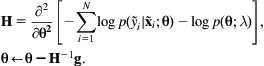
Alternatively, gradient descent can be based on the second derivative by computing the Hessian matrix H at each iteration and replacing the above update by

$\begin{array}{l}\mathbf{H}=\frac{{\partial }^2}{\partial {\mathbf{\theta }}^{\mathbf{2}}}\left[-\sum _{i=1}^N\log p({\tilde{y}}_i|{\tilde{\mathbf{x}}}_i;\mathbf{\theta })-\log p(\mathbf{\theta };\lambda )\right],\hfill \\ \mathbf{\theta }\leftarrow \mathbf{\theta }\mathbf{-}{\mathbf{H}}^{-1}\mathbf{g}.\hfill \end{array}$

Generalized Linear Models

Linear regression and logistic regression are special cases of a family of conditional probability models known in statistics as “generalized linear models,” which were proposed to unify and generalize linear and logistic regression. In this formulation, linear models may be related to a response variable using distributions other than the Gaussian distribution used for linear regression. Generalized linear models can be created for any distribution in the exponential family (Appendix A.2 introduces exponential-family distributions).

In this context, the data can be thought of in terms of response variables y_i and explanatory variables organized as p-dimensional vectors x_i, i=1,…, n. Response variables can be expressed in different ways, ranging from binary to categorical or ordinal data. A model is then defined where the expected value $E\left[y\right]$ of the distribution used for the response variable consists of an initial linear prediction ${\eta }_i={\mathbf{\beta }}^T{\mathbf{x}}_i$ using a parameter vector $\mathbf{\beta }$, which is then subjected to a smooth, invertible, and potentially nonlinear transformation using the mean function g⁻¹:

${\mu }_i=E\left[y_i\right]=g^{-1}({\mathbf{\beta }}^T{\mathbf{x}}_i).$

The mean function is the inverse of the link function g. In generalized linear modeling the entire set of explanatory variables for all the observations is arranged as an $n\times p$ matrix X, so that a vector of linear predictions for the entire data set is $\mathbf{\eta }=\mathbf{X}\mathbf{\beta }$. The variance of the underlying distribution can also be modeled; typically as a function of the mean. Different distributions, link functions, and corresponding mean functions give a great deal of flexibility in defining probabilistic models; Table 9.2 shows some examples.

Table 9.2

Link Functions, Mean Functions, and Distributions Used in Generalized Linear Models

Link Name	Link Function $\eta ={\mathbf{\beta }}^T\mathbf{x}=g(\mu )$	Mean Function $\mu =g^{-1}({\mathbf{\beta }}^T\mathbf{x})=g^{-1}(\eta )$	Typical Distribution
Identity	$\eta =\mu$	$\mu =\eta$	Gaussian
Inverse	$\eta ={\mu }^{-1}$	$\mu ={\eta }^{-1}$	Exponential
Log	$\eta ={\log }_e\mu$	$\mu =\exp (\eta )$	Poisson
Log-log	$\eta =-\log (-{\log }_e\mu )$	$\mu =\exp (-\exp (-\eta ))$	Bernoulli
Logit	$\eta ={\log }_e\frac{\mu }{1-\mu }$	$\mu =\frac{1}{1+\exp (-\eta )}$	Bernoulli
Probit	$\eta ={\Phi }^{-1}(\mu )$	$\mu =\Phi (\eta )$	Bernoulli

Note: $\mathrm{\Phi }(\cdot )$ is the cumulative normal distribution.

The multiclass extension of logistic regression discussed above is another example of a generalized linear model that uses the multinomial distribution for the response variable y. Because this model is defined in terms of probability distributions, the parameters can be estimated using maximum likelihood techniques.

Since these models are fairly simple, the coefficients ${\beta }_j$ are interpretable. Applied statisticians are often interested not only in the estimated values but in other information such as the standard error of the estimates and statistical significance tests.

Making Predictions for Ordered Classes

In many situations class values are categorical but possess a natural ordering. To deal with ordinal class attributes, the class probabilities can be expressed in terms of cumulative distributions, which are then modeled to construct an underlying probability distribution function for each class. To define a model with M ordinal categories, M–1 cumulative probability models of the form $P(Y_i\le j)$ are used for the random variable Y_i that represents the category of a given instance i. Models for $P(Y_i=j)$ are then obtained using differences between the cumulative distribution models. Here we will use complementary cumulative probabilities, known as survival functions, of the form $P(Y_i>j)=1-P(Y_i\le j)$, because this sometimes simplifies the interpretation of parameters. Then the class probabilities are obtained by:

$\begin{array}{l}P(Y_i=1)=1-P(Y_i>1)\hfill \\ P(Y_i=j)=P(Y_i>j-1)-P(Y_i>j)\hfill \\ P(Y_i=M)=P(Y_i>M-1).\hfill \end{array}$

The generalized linear models discussed above can be further generalized to ordinal categorical data. In fact, the general approach can be applied to various model classes by modeling complementary cumulative probabilities with a smooth and invertible link function that transforms them nonlinearly and equates the result to a linear predictor. For binary predictions, the models often take this form:

$\mathrm{logit}({\gamma }_{ij})=\log \frac{{\gamma }_{ij}}{1-{\gamma }_{ij}}=b_j+{\mathbf{w}}^T{\mathbf{x}}_i,$

where w is a vector of weights, x_i are vectors of features, and ${\gamma }_{ij}$ represent the probability that example i is greater than the discretized, ordinal category j. Such models are called “proportional odds” models, or “ordered logit” models. The model above uses a different bias for each inequality, but the same set of weights. This guarantees a consistent set of probabilities.

Conditional Probabilistic Models Using Kernels

Linear models can be transformed into nonlinear ones by applying the “kernel trick” mentioned in Section 7.2 under kernel regression, or, alternatively, through basis expansion as mentioned in the section above on matrix formulations of linear and polynomial regression. This can be applied to both kernel regression and kernel logistic regression.

Suppose the features x are replaced by the vector k(x) whose elements are determined using a kernel function k(x,x_j) for every training example (or for some subset of training vectors):

$\mathbf{k}(\mathbf{x})=\left[\begin{array}{c}k(\mathbf{x},{\mathbf{x}}_1)\\ ⋮\\ k(\mathbf{x},{\mathbf{x}}_V)\\ 1\end{array}\right]$

A “1” has been appended to this vector to implement the bias term in the parameter matrix. A kernel regression is then

$p(y|\mathbf{x})=N(y;{\mathbf{w}}^T\mathbf{k}(\mathbf{x}),{\sigma }^2).$

For classification, an analogous kernel logistic regression is

$p(\mathbf{y}|\mathbf{x})=\frac{\exp ({\mathbf{y}}^T\mathbf{\theta }\mathbf{k}(\mathbf{x}))}{\sum _{\mathbf{y}}\exp ({\mathbf{y}}^T\mathbf{\theta }\mathbf{k}(\mathbf{x}))}=\frac{1}{Z(\mathbf{k}(\mathbf{x}))}\exp ({\mathbf{y}}^T\mathbf{\theta }\mathbf{k}(\mathbf{x})).$

Since every example in the training set can have a different kernel vector, it is necessary to compute a kernel matrix K with entries given by K_ij=k(x_i,x_j). For large datasets this operation can be time- and memory-intensive.

Support vector machines have a similar form, although they are not formulated probabilistically, and multiclass support vector machines are not as easily formulated as multiclass kernel logistic regression. Because they use an underlying hinge loss and weight regularization term, support vector machines often assign zero weights to many of the terms; they also have the appealing feature of placing nonzero weights only on vectors that reside at the boundary of the decision surface. In many applications this results in a significant reduction in the number of kernel evaluations needed at test time. Neither kernel logistic regression nor kernel ridge regression produce such sparse solutions, even when a Gaussian or (squared) L₂ regularization is used: in general there is a nonzero weight for every exemplar. However, kernel logistic regression can outperform support vector machines, and several techniques have been proposed to make these methods sparse. They are mentioned in the Further Reading section at the end of the chapter.

Markov Models and N-gram Methods

One simple and effective probabilistic model for discrete sequential data is known as a “Markov model.” A first-order Markov model assumes that each symbol in a sequence can be predicted using its conditional probability given the preceding symbol. (For the very first symbol, an unconditional probability is used.) Given observation variables O={O₁,…,O_T}, this can be written

$P(\mathrm{O})=P(O_1)\prod _{t=1}^{T}P(O_{t+1}|O_t).$

Usually, every conditional probability used in such models is the same. The corresponding Bayesian networks consist simply of a linear chain of variables with directed edges between each successive pair; Fig. 9.18A shows an example. The method generalizes naturally to second-order models (Fig. 9.18B), and to higher orders. N-gram models correspond to the use of an (N–1)-th order Markov model. For example, first-order models involve the use of 2-grams (or “bigrams”); third-order models use trigrams, and zero-th order models correspond to single observations or “unigrams.” Such models are widely used for modeling biological sequences such as DNA, as well as for text mining and computational linguistics applications.

All probabilistic models raise the issue of what to do when there is no data for certain configurations of variables. Zero-valued parameters cause problems, as we saw in Section 4.2. This is particularly severe with high-order Markov models, and smoothing techniques—such as Laplace or Dirichlet smoothing, which can be derived from a Bayesian analysis—become critical. See the Further Reading section for some pointers to some specialized methods for smoothing n-grams.

Large n-gram models are extremely useful for applications ranging from machine translation and speech recognition to spelling correction and information extraction. Indeed, Google has made available English language word counts for a billion five-word sequences that appear at least 40 times in a trillion-word corpus After discarding words that appear less than 200 times, there remain 13 million unique words (unigrams), 300 million bigrams; and around a billion each of trigrams, four-grams, and five-grams.

Hidden Markov Models

Hidden Markov models have been widely used for pattern recognition since at least the 1980s. Until recently most of the major speech recognition systems have consisted of large Gaussian mixture models combined with hidden Markov models. Many problems in biological sequence analysis can also be formulated in terms of hidden Markov models, with various extensions and generalizations.

A hidden Markov model is a joint probability model of a set of discrete observed variables O={O₁,…,O_T} and discrete hidden variables H={H₁,…,H_T} for T observations that factors the joint distribution as follows:

$P(\mathrm{O},\mathrm{H})=P(H_1)\prod _{t=1}^{T}P(H_{t+1}|H_t)\prod _{t=1}^{T}P(O_t|H_t),$

Each O_t is a discrete random variable with N possible values, and each H_t is a discrete random variable with M possible values. Fig. 9.18C illustrates a hidden Markov model as a type of Bayesian network that is known as a “dynamic” Bayesian network because variables are replicated dynamically over the appropriate number of time steps. They are an obvious extension of first-order Markov models, and it is common to use “time-homogeneous” models where the transition matrix P(H_t+1|H_t) is the same at each time step. Define A to be a transition matrix whose elements encode P(H_t+1=j|H_t=i), and B to be an emission matrix B whose elements b_ij correspond to P(O_t=j|H_t=i). For the special t=1 the initial state probability distribution is encoded in a vector π with elements π_i=P(H_t=i). The complete set of parameters is $\theta =\{\mathbf{A},\mathbf{B},\mathbf{\pi }\}$, a set containing two matrices and one vector. We write a particular observation sequence as a set of observations $\tilde{\mathrm{O}}=\{O_1=o_1,\dots ,O_T=o_T\}$.

Hidden Markov models pose three key problems:

The first problem can be solved using the sum-product algorithm, the second using the max-product algorithm, and the third using the EM algorithm for which the required expectations are computed using the sum-product algorithm. If there is labeled data for the sequences of hidden variables that correspond to observed sequences, the required conditional probability distributions can be computed from the corresponding counts in the same way as we did with Bayesian networks.

The only difference between the parameter estimation task when using an hidden Markov model viewed as a dynamic Bayesian network and the updates used for learning the conditional probability tables in a Bayesian network is that one can average over the statistics obtained at each time step, because the same emission and transition matrices are used at each step. The basic hidden Markov model formulation serves as a point of reference when coupling more complex probabilistic models over time using more general dynamic Bayesian network models.

Conditional Random Fields

Hidden Markov models are not the only models that are useful when working with sequence data. Conditional random fields are a statistical modeling technique that takes context into account, and are often structured as linear chains. They are widely used for sequence processing tasks in data mining, but are also popular in image processing and computer vision. Fig. 9.19 illustrates the problem of extracting locations and dates of meetings from email text, which can be addressed using chain-structured conditional random fields. A major advantage is that these models can be given arbitrarily complex features of the input sequence to be used for making predictions—e.g., matching words to lists of organizations and processing variations of known abbreviations.

Inference for chain-structured conditional random fields can be performed efficiently using the sum- and max-product algorithms discussed above. The sum-product algorithm can be used to compute the expected gradients needed to learn them, and the max-product algorithm serves to label new sequences—with tags such as “where” indicating the location or room and “time” labels associated with a meeting.

We begin with a general definition, and then focus on the simpler case of linear conditional random fields. Fig. 9.20D shows a chain-structured conditional random field, illustrated as a factor graph, which can be contrasted with the Markov random field depicted in Fig. 9.20B and the hidden Markov model in Fig. 9.20C, also shown as a factor graph. Circles are not used to represent the observed variables in Fig. 9.20D because the underlying conditional random field model does not explicitly encode these as random variables in the graph.

From Markov random fields to conditional random fields

Whereas both Bayesian networks and Markov random fields define a joint probability model for data, conditional random fields (also known as “structured prediction” techniques) define a joint conditional distribution for multiple predictions. For a set X of random variables, we have already seen how a Markov random field factorizes the joint distribution for X using an exponentiated energy function F(X):

$\begin{array}{l}P(X)=\frac{1}{Z}\exp (-F(X)),\hfill \\ Z=\sum _X\exp (-F(X)),\hfill \end{array}$

where the sum is over all states of all variables in X. Conditional random fields condition on some observations, yielding a conditional distribution:

$\begin{array}{l}P(Y|X)=\frac{1}{Z(X)}\exp (-F(Y,X)),\hfill \\ Z(X)=\sum _Y\exp (-F(Y,X)),\hfill \end{array}$

where the sum is over all states of all variables in Y. Both Markov and conditional random fields can be defined for general model structures, but the energy functions usually include just one or two variables—unary and pairwise potentials. Conceptually, to create a conditional random field for P(Y|X) based on U unary and V pairwise functions of variables in Y, the energy function takes the form

$F(Y,\tilde{X})=\sum _{u=1}^{U}U(Y_u,\tilde{X})+\sum _{v=1}^{V}V(Y_v,\tilde{X}).$

Such energy functions can be transformed into so-called potential functions by negation, exponentiation, and normalization. The conditional probability model takes this form:

$\begin{array}{ll}P(Y|\tilde{X})\hfill & =\frac{1}{Z(\tilde{X})}\exp \left[\sum _{u=1}^{U}U(Y_u,\tilde{X})+\sum _{v=1}^{V}V(Y_v,\tilde{X})\right]\hfill \\ \hfill & =\frac{1}{Z(\tilde{X})}\prod _{u=1}^U{\varphi }_u(Y_u,\tilde{X})\prod _{v=1}^V{\mathrm{\Psi }}_v(Y_v,\tilde{X}).\hfill \end{array}$ (9.8)

(9.8)

Lattice-structured models like this are used in image processing applications, as mentioned earlier. Processing sequences with chain-structured conditional random fields is even simpler. Note that logistic regression could be thought of as a simple conditional random field, one that arises naturally from a conditional version of a Markov random field with a factorization shown in Fig. 9.15B.

Linear chain conditional random fields

Consider observations $\tilde{Y}=\{y_1={\tilde{y}}_1,\dots ,y_N={\tilde{y}}_N\}$ of a sequence of discrete random variables $Y=\{y_1,\dots ,y_N\}$, using integers to encode the relevant states, and an observed input sequence $\tilde{X}=\{{\tilde{x}}_1,\dots ,{\tilde{x}}_N\}$, which can be of any data type. A conditional random field defines the conditional probability $P(Y|X)$ of a label sequence given an input sequence. This contrasts with hidden Markov models, which treat both Y and X as random variables and defines a joint probability model for P(Y,X). Note that X above was intentionally not defined as a sequence of random variables because we will define the conditional distribution of Y given X and need not have an explicit model for P(X). Of course, an implicit model for P(X) could be defined as the empirical distribution of the data, or the distribution produced by placing a Dirac or Kronecker delta function on each observation and normalizing by the number of examples. Not defining X as a sequence leaves open what type of variables these are, and whether it is just a set of variables or a set of formally defined random variables. Fig. 9.20D uses shaded rectangles to emphasize this point. In this chain model, for a given sequence of length N, Eq. (9.8) could be re-written

$P(Y|\tilde{X})=\frac{1}{Z(\tilde{X})}\prod _{u=1}^N{\varphi }_u(y_u,\tilde{X})\prod _{v=1}^N{\mathrm{\Psi }}_v(y_v,y_{v+1},\tilde{X}).$

Focusing on a linear chain structure reveals some analogies with the emission and transition matrices of hidden Markov models. There are two types of features: a set of J single variable (state) features $u_j(y_{\mathrm{i}},X,i)$ that are a function of a single y_i, and which are computed for each y_i in the sequence i=1,…, N; and a set of K pairwise (transition) features $v_k(y_{i-1},y_i,X,i)$ for i>1. Each type has associated unary weights ${\theta }_{\mathrm{j}}^{\mathrm{u}}$ and pairwise weights ${\theta }_k^v$. Note that these features can be a function of the entire observed sequence $\tilde{X}$, or of some subset. This global dependence on the input is a major advantage of conditional random fields over hidden Markov models. The analog of the Markov model transition matrix are the per-position pairwise potential functions: these can be written as a set of matrices that depend upon the observation sequence and consist of a sum over the product of pairwise weights ${\theta }_{\mathrm{k}}^{\mathrm{v}}$ and pairwise features

${\mathrm{\Psi }}_i[y_i,y_{i+1}]=\exp \left[\sum _{k=1}^{\mathrm{K}}{\theta }_k^v{v}_k(y_i,y_{i+1},\tilde{X},i)\right].$

The unary potential functions play a similar role to the terms arising from the hidden Markov model emission matrices, and can be written as the following set of vectors that involve exponentiated weighted combinations of unary features

${\mathbf{\varphi }}_i\left[y_i\right]=\exp \left[\sum _{j=1}^J{\theta }_j^u{u}_j(y_i,\tilde{X},i)\right].$

Sometimes, rather than keeping the unary and pairwise features and their parameters separate, it is useful to work with all features for a given position i. To do this, define $\mathbf{f}(y_i,y_{i+1},X,i)$ as a length-L vector containing all single-variable and pairwise features, and define the global feature vector to be the sum over each of these position dependent feature vectors:

$\mathbf{g}(Y,X)=\sum _{i=1}^N\mathbf{f}(y_i,y_{i+1},X,i).$

Now a conditional random field can be written in a particularly compact form

$P(Y|X)=\frac{\exp ({\mathbf{\theta }}^T\mathbf{g}(Y,X))}{\sum _Y\exp ({\mathbf{\theta }}^T\mathbf{g}(Y,X))}.$

If we turn to the problem of learning based on maximizing the conditional likelihood for this model, an analogy can be drawn to the simpler case of logistic regression. The gradient of the log-likelihood of a conditional random field for a set of M input sequences $A=\{{\tilde{X}}_1,\dots ,{\tilde{X}}_M\}$ and corresponding output sequences $B=\{{\tilde{Y}}_1,\dots ,{\tilde{Y}}_M\}$, is

$\frac{\partial }{\partial \mathbf{\theta }}\log P(B|A)=\sum _{m=1}^M[\mathbf{g}({\tilde{Y}}_m,{\tilde{X}}_m)-E_m[\mathbf{g}(Y_m,{\tilde{X}}_m)\left]\right].$

Here, E_m[.] is an expectation taken with respect to $P(Y_m|{\tilde{X}}_m)$. It is standard practice to include a Gaussian prior or L₂ regularization on parameters by adding a regularization term to this expression. Unlike logistic regression, this expectation involves the joint distribution of the label sequence and not just the distribution for a single label variable. However, in chain-structured graphs it can be computed efficiently and exactly using the sum-product algorithm.

Learning for chain-structured conditional random fields

To compute the gradient for a linear chain conditional random field, it is useful to expose each parameter in the L₂ regularized log-likelihood in scalar form:

$\log P(B|A)=\sum _{m=1}^M\sum _{i=1}^{N_m}\sum _{l=1}^L{\theta }_l{g}_l({\tilde{y}}_{m,i},{\tilde{y}}_{m,i+1},{\tilde{X}}_m)-\sum _{m=1}^M\log Z({\tilde{X}}_m)-\sum _{l=1}^L\frac{{\theta }_l^2}{2{\sigma }^2}.$

where σ is the regularization parameter. Taking the derivative with respect to a single parameter and training example, the contribution to the gradient of each example is

$\frac{\partial }{\partial {\theta }_l}\log P({\tilde{Y}}_m|{\tilde{X}}_m)=\sum _{i=1}^{N_m}{g}_l({\tilde{y}}_i,{\tilde{y}}_{i+1},\tilde{X})-\sum _{i=1}^{N_m}\sum _{y_i}\sum _{y_{i+1}}{g}_l(y_i,y_{i+1},\tilde{X})P(y_i,y_{i+1}|\tilde{X})-\frac{{\theta }_l}{{\sigma }^2}.$

This is simply the difference between the observed occurrence of the feature and its expectation under the current prediction of the model, taken with respect to $P(y_i,y_{i+1}|\tilde{X})$, minus the partial derivative of the regularization term. Similar terms arise for unary functions, but the expectation is taken with respect to $P(y_i|\tilde{X})$. These distributions are the single- and pairwise-variable marginal conditional distributions, and can be computed efficiently using the sum-product algorithm.

Software Packages and Implementations

Implementations of principal component analysis, Gaussian mixture models, and hidden Markov models are widely available in many software packages. MatLab’s statistics toolbox, e.g., has implementations of principal component analysis and its probabilistic variant based on the methods we have discussed, and also contains implementations of Gaussian mixture models and all the canonical hidden Markov model manipulations.

Kevin Murphy’s MatLab-based Probabilistic Modeling Toolkit is a large, open source collection of MatLab functions and tools. The software contains implementations for many of the methods we have discussed here, including code for Bayesian network manipulation and inference methods.

The Hugin software package from Hugin Expert A/S and the Netica software from Norsys are well-known commercial software implementations for manipulating Bayesian networks. They contain excellent graphical user interfaces for interacting with these networks.

The BUGS (Bayesian inference Using Gibbs Sampling) project has created a variety of software packages for the Bayesian analysis of complex statistical models using Markov chain Monte Carlo methods. WinBUGS (Lunn et al., 2000) is a stable version of the software, but the more recent OpenBUGS project is an open source version of the core BUGS implementation (Lunn, Spiegelhalter, Thomas, & Best, 2009).

The VIBES software package (Bishop, Spiegelhalter, & Winn, 2002) allows inference in graphical models using variational methods. Microsoft Research has created a programming language known as infer.net that allows one to define graphical models and perform inference in them using variational methods, Gibbs sampling or another message passing method known as expectation propagation (Minka, 2001). Expectation propagation generalizes belief propagation to distributions and models beyond the typical discrete and binary models used to create Bayesian networks. John Winn and Tom Minka at Microsoft Research have been leading the infer.net project.

The R programming language and software environment was created for statistical computing and visualization (Ihaka & Gentleman, 1996). It has its origins at the University of Auckland, and provides an open source implementation of the S programming language from Bell Labs. It is comparable to well known commercial packages such as SAS, SPSS, and Stata, and contains implementations of many classical statistical methods such as generalized linear models and other regression techniques. Since it is a general purpose programming language there are many extensions and implementations of the models discussed in this chapter available online. Historically Brian D. Ripley has overseen the development of R. Ripley is now retired from Oxford University where he was a statistic Professor. He is the coauthor of a number of books on S programming (Venables & Ripley, 2000, 2002) and an older but very high-quality textbook on pattern recognition and neural networks (Ripley, 1996).

The MALLET Machine Learning for Language Toolkit (McCallum, 2002) provides excellent Java implementations of latent Dirichlet allocation and conditional random fields. It also provides many other statistical natural language-processing methods ranging from document classification and clustering to topic modeling, information extraction, and other machine learning techniques frequently used for text processing.

The open source Alchemy software package is widely used for Markov logic networks (Richardson & Domingos, 2006).

Scikit-learn (Pedregosa et al., 2011) is a rapidly growing Python-based set of implementations of many machine learning methods. It contains implementations of many probabilistic and statistical methods for classification, regression, clustering, dimensionality reduction (including factor analysis and PPCA), model selection and preprocessing.