
Probabilistic methods
Abstract
It is now time to introduce probabilistic approaches to data mining and machine learning in a formal way. We begin by outlining fundamental aspects of probability theory that are widely used in data mining and practical machine learning. The maximum likelihood approach is presented, along with methods for learning with hidden variables, including the well-known expectation maximization algorithm. Maximum likelihood methods are cited in the context of approaches that are more Bayesian in nature, and the role of variational methods and sampling procedures are also discussed. Bayesian networks are presented and used to describe a wide variety of methods, such as mixture models, principal component analysis, and latent Dirichlet allocation, as well as other probabilistic methods. Conditional probability models are discussed, including key derivations for regression and multiclass classification. Their relationships to widely used generalized linear models are also outlined. Methods for modeling and extracting information from sequences and for structured prediction problems are also presented, including Markov models, hidden Markov models, Markov random fields, and conditional random fields. Software packages that specialize in creating and using these models and methods are also surveyed.
Keywords
Probability theory; maximum likelihood; hidden variables; expectation maximization (EM); variational methods; sampling procedures; Bayesian networks; mixture models; principal component analysis; latent Dirichlet allocation; Markov models; hidden Markov models; random fields
Probabilistic methods form the basis of a plethora of techniques for data mining and machine learning. In Section 4.2, “Simple probabilistic modeling,” we encountered the idea of choosing a model that maximizes the likelihood of an event, and have referred to the general idea of maximizing likelihoods several times since. In this chapter we will formalize the notion of likelihoods, and see how maximizing them underpins many estimation problems. We will look at Bayesian networks, and other types of probabilistic models used in machine learning. Let us begin by establishing the foundations: some fundamental rules of probability.
9.1 Foundations
In probability modeling, example data or instances are often thought of as being events, observations, or realizations of underlying random variables. Given a discrete random variable A, P(A) is a function that encodes the probabilities for each of the categories, classes, or states that A may be in. Similarly, for continuous random variables x, p(x) is a function that assigns a probability density to all possible values of x. In contrast, P(A=a) is the single probability of observing the specific event A=a. This notation is often simplified to P(a), but one needs to be careful to remember whether a was defined as a random variable or as an observation. Similarly for the observation that continuous random variable x has the value x1: it is common to write this probability density as p(x1), but this is a simplification of the longer but clearer notation ![]() , which emphasizes that it is the scalar value obtained by evaluating the function at x=x1.
, which emphasizes that it is the scalar value obtained by evaluating the function at x=x1.
There are a few rules of probability theory that are particularly relevant to this book. They go by various names, but we will refer to them as the product rule, the sum (or marginalization) rule, and Bayes’ rule. As we will see, these seemingly simple rules can take us far.
Discrete or binary events are used below to keep the notation simple. However, the rules can be applied to binary, discrete, or continuous events and variables. For continuous variables, sums over possible states are replaced by integrals.
The product rule, sometimes referred to as the “fundamental rule of probability,” states that the joint probability of random variables A and B can be written
The product rule also applies when A and B are groups or subsets of events or random variables.
The sum rule states that given the joint probability of variables X1, X2,…, XN, the marginal probability for a given variable can be obtained by summing (or integrating) over all the other variables. For example, to obtain the marginal probability of X1, sum over all the states of all the other variables:
The sums are taken over all possible values for the corresponding variable. This notation can be simplified by writing
For continuous events and variables x1, x2,…, xN, the equivalent formulation is obtained by integrating rather than summing:
This can give the marginal distribution of any random variable, or of any subset of random variables.
The famous Bayes’ rule that was introduced in Chapter 4, Algorithms: the basic methods, can be obtained from the product rule by swapping A and B, observing that ![]() , and rearranging:
, and rearranging:
Suppose we have models for ![]() and
and ![]() , observe that event A=a, and want to compute
, observe that event A=a, and want to compute ![]() .
. ![]() is referred to as the likelihood,
is referred to as the likelihood, ![]() as the prior distribution of B, and
as the prior distribution of B, and ![]() as the posterior distribution.
as the posterior distribution. ![]() is obtained from the sum rule:
is obtained from the sum rule:
These concepts can be applied to random variables, and also to parameters when they are treated as random quantities.
Maximum Likelihood Estimation
Consider the problem of estimating a set of parameters θ of a probabilistic model, given a set of observations x1, x2,…, xn. Assume they are continuous-valued observations—but the same idea applies to discrete data too. Maximum likelihood techniques assume that (1) the examples have no dependence on one another, in that the occurrence of one has no effect on the others, and (2) they can each be modeled in exactly the same way. These assumptions are often summarized by saying that events are independent and identically distributed (i.i.d.). Although this is rarely completely true, it is sufficiently true in many situations to support useful inferences. Furthermore, as we will see later in this chapter, dependency structure can be captured by more sophisticated models—e.g., by treating interdependent groups of observations as part of a larger instance.
The i.i.d. assumption implies that a model for the joint probability density function for all observations consists of the product of the same probability model p(xi;θ) applied to each observation independently. For n observations, this could be written
Each function p(xi;θ) has the same parameter values θ, and the aim of parameter estimation is to maximize a joint probability model of this form. Since the observations do not change, this value can only be changed by altering the choice of the parameters θ. We can think about this value as the likelihood of the data, and write it as
Since the data is fixed, it is arguably more useful to think of this as a likelihood function for the parameters, which we are free to choose.
Multiplying many probabilities can lead to very small numbers, and so people often work with the logarithm of the likelihood, or log-likelihood:
which converts the product into a sum. Since logarithms are strictly monotonically increasing functions, maximizing the log-likelihood is the same as maximizing the likelihood. “Maximum likelihood” learning refers to techniques that search for parameters that do this:
The same formulation also works for conditional probabilities and conditional likelihoods. Given some labels yi that accompany each xi, e.g., class labels of instances in a classification task, maximum conditional likelihood learning corresponds to determining
Maximum a Posteriori Parameter Estimation
Maximum likelihood assumes that all parameter values are equally likely a priori: we do not judge some parameter values to be more likely than others before we have considered the observations. But suppose we have reason to believe that the model’s parameters follow a certain prior distribution. Thinking of them as random variables that specify each instance of the model, Bayes’ rule can be applied to compute a posterior distribution of the parameters using the joint probability of data and parameters:
Since we are computing the posterior distribution over the parameters, we have used | or the “given” notation in place of the semicolon. The denominator is a constant, and assuming i.i.d. observations, the posterior probability of the parameters is proportional to the product of the likelihood and prior:
Switching to logarithms again, the maximum a posteriori parameter estimation procedure seeks a value
Again, the same idea can be applied to learn conditional probability models.
We have reverted to the semicolon notation to emphasize that maximum a posteriori parameter estimation involves point estimates of the parameters, evaluating them under the likelihood and prior distributions. This contrasts with fully Bayesian methods (discussed below) that explicitly manipulate the distribution of the parameters, typically by integrating over the parameter’s uncertainty instead of optimizing a point estimate. The use of the “given” notation in place of the semicolon is more commonly used with fully Bayesian methods, and we will follow this convention.
9.2 Bayesian Networks
The Naïve Bayes classifier of Section 4.2 and the logistic regression models of Section 4.6 both produce probability estimates rather than hard classifications. For each class value, they estimate the probability that a given instance belongs to that class. Most other types of classifiers can be coerced into yielding this kind of information if necessary. For example, probabilities can be obtained from a decision tree by computing the relative frequency of each class in a leaf and from a decision list by examining the instances that a particular rule covers.
Probability estimates are often more useful than plain predictions. They allow predictions to be ranked, and their expected cost to be minimized (see Section 5.8). In fact, there is a strong argument for treating classification learning as the task of learning class probability estimates from data. What is being estimated is the conditional probability distribution of the values of the class attribute given the values of the other attributes. Ideally, the classification model represents this conditional distribution in a concise and easily comprehensible form.
Viewed in this way, Naïve Bayes classifiers, logistic regression models, decision trees, and so on are just alternative ways of representing a conditional probability distribution. Of course, they differ in representational power. Naïve Bayes classifiers and logistic regression models can only represent simple distributions, whereas decision trees can represent—or at least approximate—arbitrary distributions. However, decision trees have their drawbacks: they fragment the training set into smaller and smaller pieces, which inevitably yield less reliable probability estimates, and they suffer from the replicated subtree problem described in Section 3.4. Rule sets go some way toward addressing these shortcomings, but the design of a good rule learner is guided by heuristics with scant theoretical justification.
Does this mean that we have to accept our fate and live with these shortcomings? No! There is a statistically based alternative: a theoretically well-founded way of representing probability distributions concisely and comprehensibly in a graphical manner. The structures are called Bayesian networks. They are drawn as a network of nodes, one for each attribute, connected by directed edges in such a way that there are no cycles—a directed acyclic graph.
In this section, to explain how to interpret Bayesian networks and how to learn them from data we will make some simplifying assumptions. We assume that all attributes are nominal—they correspond to discrete random variables—and that there are no missing values, so the data is complete. Some advanced learning algorithms can create new attributes in addition to the ones present in the data—so-called hidden attributes corresponding to latent variables whose values cannot be observed. These can support better models if they represent salient features of the underlying problem, and Bayesian networks provide a good way of using them at prediction time. However, they make both learning and prediction far more complex and time consuming, so we will defer considering them to Section 9.4.
Making Predictions
Fig. 9.1 shows a simple Bayesian network for the weather data. It has a node for each of the four attributes outlook, temperature, humidity, and windy and one for the class attribute play. An edge leads from the play node to each of the other nodes. But in Bayesian networks the structure of the graph is only half the story. Fig. 9.1 shows a table inside each node. The information in the tables defines a probability distribution that is used to predict the class probabilities for any given instance.

Before looking at how to compute this probability distribution, consider the information in the tables. The lower four tables (for outlook, temperature, humidity, and windy) have two parts separated by a vertical line. On the left are the values of play, and on the right are the corresponding probabilities for each value of the attribute represented by the node. In general, the left side contains a column for every edge pointing to the node, in this case just an edge emanating from the node for the play attribute. That is why the table associated with play itself does not have a left side: it has no parents. In general, each row of probabilities corresponds to one combination of values of the parent attributes, and the entries in the row show the probability of each value of the node’s attribute given this combination. In effect, each row defines a probability distribution over the values of the node’s attribute. The entries in a row always sum to 1.
Fig. 9.2 shows a more complex network for the same problem, where three nodes (windy, temperature, and humidity) have two parents. Again, there is one column on the left for each parent and as many columns on the right as the attribute has values. Consider the first row of the table associated with the temperature node. The left side gives a value for each parent attribute, play and outlook; the right gives a probability for each value of temperature. For example, the first number (0.143) is the probability of temperature taking on the value hot, given that play and outlook have values yes and sunny, respectively.

How are the tables used to predict the probability of each class value for a given instance? This turns out to be very easy, because we are assuming that there are no missing values. The instance specifies a value for each attribute. For each node in the network, look up the probability of the node’s attribute value based on the row determined by its parents’ attribute values. Then just multiply all these probabilities together.
For example, consider an instance with values outlook=rainy, temperature=cool, humidity=high, and windy=true. To calculate the probability for play=no, observe that the network in Fig. 9.2 gives probability 0.367 from node play, 0.385 from outlook, 0.429 from temperature, 0.250 from humidity, and 0.167 from windy. The product is 0.0025. The same calculation for play=yes yields 0.0077. However, these are clearly not the final answer: the final probabilities must sum to 1, whereas 0.0025 and 0.0077 do not. They are actually the joint probabilities ![]() and
and ![]() , where E denotes all the evidence given by the instance’s attribute values. Joint probabilities measure the likelihood of observing an instance that exhibits the attribute values in E as well as the respective class value. They only sum to 1 if they exhaust the space of all possible attribute–value combinations, including the class attribute. This is certainly not the case in our example.
, where E denotes all the evidence given by the instance’s attribute values. Joint probabilities measure the likelihood of observing an instance that exhibits the attribute values in E as well as the respective class value. They only sum to 1 if they exhaust the space of all possible attribute–value combinations, including the class attribute. This is certainly not the case in our example.
The solution is quite simple (we already encountered it in Section 4.2). To obtain the conditional probabilities ![]() and
and ![]() , normalize the joint probabilities by dividing them by their sum. This gives probability 0.245 for play=no and 0.755 for play=yes.
, normalize the joint probabilities by dividing them by their sum. This gives probability 0.245 for play=no and 0.755 for play=yes.
Just one mystery remains: Why multiply all those probabilities together? It turns out that the validity of the multiplication step hinges on a single assumption—namely that, given values for each of a node’s parents, knowing the values for any other set of nondescendants does not change the probability associated with each of its possible values. In other words, other sets of nondescendants do not provide any information about the likelihood of the node’s values over and above the information provided by the parents. This can be written
which must hold for all values of the nodes and attributes involved. In statistics this property is called conditional independence. Multiplication is valid provided that each node is conditionally independent of its grandparents, great grandparents, and indeed any other set of nondescendants, given its parents. We have discussed above how the product rule of probability can be applied to sets of variables. Applying the product rule recursively between a single variable and the rest of the variables gives rise to another rule known as the chain rule which states that the joint probability of n attributes Ai can be decomposed into the following product:
The multiplications of probabilities in Bayesian networks follow as a direct result of the chain rule.
The decomposition holds for any order of the attributes. Because our Bayesian network is an acyclic graph, its nodes can be ordered to give all ancestors of a node ai indices smaller than i. Then, because of the conditional independence assumption all Bayesian networks can be written in the form
where when a variable has no parents, we use the unconditional probability of that variable. This is exactly the multiplication rule that we applied earlier.
The two Bayesian networks in Figs. 9.1 and 9.2 are fundamentally different. The first (Fig. 9.1) makes stronger independence assumptions because for each of its nodes the set of parents is a subset of the corresponding set of parents in the second (Fig. 9.2). In fact, Fig. 9.1 is almost identical to the simple Naïve Bayes classifier of Section 4.2 (The probabilities are slightly different but only because each count has been initialized to 0.5 to avoid the zero-frequency problem.) The network in Fig. 9.2 has more rows in the conditional probability tables and hence more parameters; it may be a more accurate representation of the underlying true probability distribution that generated the data.
It is tempting to assume that the directed edges in a Bayesian network represent causal effects. But be careful! In our case, a particular value of play may enhance the prospects of a particular value of outlook, but it certainly does not cause it—it is more likely to be the other way round. Different Bayesian networks can be constructed for the same problem, representing exactly the same probability distribution. This is done by altering the way in which the joint probability distribution is factorized to exploit conditional independencies. The network whose directed edges model causal effects is often the simplest one with the fewest parameters. Hence, human experts who construct Bayesian networks for a particular domain often benefit by representing causal effects by directed edges. However, when machine learning techniques are applied to induce models from data whose causal structure is unknown, all they can do is construct a network based on the correlations that are observed in the data. Inferring causality from correlation is always a dangerous business.
Learning Bayesian Networks
The way to construct a learning algorithm for Bayesian networks is to define two components: a function for evaluating a given network based on the data and a method for searching through the space of possible networks. The quality of a given network is measured by the probability of the data given the network. We calculate the probability that the network accords to each instance and multiply these probabilities together over all instances. In practice, this quickly yields numbers too small to be represented properly (called arithmetic underflow), so we use the sum of the logarithms of the probabilities rather than their product. The resulting quantity is the log-likelihood of the network given the data.
Assume that the structure of the network—the set of edges—is given. It is easy to estimate the numbers in the conditional probability tables: just compute the relative frequencies of the associated combinations of attribute values in the training data. To avoid the zero-frequency problem each count is initialized with a constant as described in Section 4.2. For example, to find the probability that humidity=normal given that play=yes and temperature=cool (the last number of the third row of the humidity node’s table in Fig. 9.2), observe from Table 1.2 that there are three instances with this combination of attribute values in the weather data, and no instances with humidity=high and the same values for play and temperature. Initializing the counts for the two values of humidity to 0.5 yields the probability (3+0.5)/(3+0+1)=0.875 for humidity=normal.
Let us consider more formally how to estimate the conditional and unconditional probabilities in a Bayesian network. The log-likelihood of a Bayesian network with V variables and N examples of complete assignments to the network is
where the parameters of each conditional or unconditional distribution are given by ![]() , and we use the ~ to indicate actual observations of a variable. We find the maximum likelihood parameter values by taking derivatives. Since the log-likelihood is a double sum over examples i and variables v, when we take the derivative of it with respect to any given set of parameters
, and we use the ~ to indicate actual observations of a variable. We find the maximum likelihood parameter values by taking derivatives. Since the log-likelihood is a double sum over examples i and variables v, when we take the derivative of it with respect to any given set of parameters ![]() , all the terms of the sum that are independent of
, all the terms of the sum that are independent of ![]() will be zero. This means that the estimation problem decouples into the problem of estimating the parameters for each conditional or unconditional probability distribution separately. For variables with no parents, we need to estimate an unconditional probability. In Appendix A.2 we give a derivation illustrating why estimating a discrete distribution with parameters given by the probabilities
will be zero. This means that the estimation problem decouples into the problem of estimating the parameters for each conditional or unconditional probability distribution separately. For variables with no parents, we need to estimate an unconditional probability. In Appendix A.2 we give a derivation illustrating why estimating a discrete distribution with parameters given by the probabilities ![]() for k classes corresponds to the intuitive formula
for k classes corresponds to the intuitive formula ![]() , where nk is the number of examples of class k and N is the total number of examples. This can also be written
, where nk is the number of examples of class k and N is the total number of examples. This can also be written
where ![]() is simply an indicator function that returns 1 when the ith observed value for
is simply an indicator function that returns 1 when the ith observed value for ![]() and 0 otherwise. The estimation of the entries of a conditional probability table for P(B|A) can be expressed using a notation similar to the intuitive counting procedures outlined above:
and 0 otherwise. The estimation of the entries of a conditional probability table for P(B|A) can be expressed using a notation similar to the intuitive counting procedures outlined above:

This derivation generalizes to the situation where A is a subset of random variables. Note that the above expressions give maximum likelihood estimates, and do not deal with the zero-frequency problem.
The nodes in the network are predetermined, one for each attribute (including the class). Learning the network structure amounts to searching through the space of possible sets of edges, estimating the conditional probability tables for each set, and computing the log-likelihood of the resulting network based on the data as a measure of the network’s quality. Bayesian network learning algorithms differ mainly in the way in which they search through the space of network structures. Some algorithms are introduced below.
There is one caveat. If the log-likelihood is maximized based on the training data, it will always be better to add more edges: the resulting network will simply overfit. Various methods can be employed to combat this problem. One possibility is to use cross-validation to estimate the goodness of fit. A second is to add a penalty for the complexity of the network based on the number of parameters, i.e., the total number of independent estimates in all the probability tables. For each table, the number of independent probabilities is the total number of entries minus the number of entries in the last column, which can be determined from the other columns because all rows must sum to 1. Let K be the number of parameters, LL the log-likelihood, and N the number of instances in the data. Two popular measures for evaluating the quality of a network are the Akaike Information Criterion (AIC):
and the following MDL metric based on the MDL principle:
In both cases the log-likelihood is negated, so the aim is to minimize these scores.
A third possibility is to assign a prior distribution over network structures and find the most likely network by combining its prior probability with the probability accorded to the network by the data. This is the maximum a posteriori approach to network scoring. Depending on the prior distribution used, it can take various forms. However, true Bayesians would average over all possible network structures rather than singling one particular network out for prediction. Unfortunately, this generally requires a great deal of computation. A simplified approach is to average over all network structures that are substructures of a given network. It turns out that this can be implemented very efficiently by changing the method for calculating the conditional probability tables so that the resulting probability estimates implicitly contain information from all subnetworks. The details of this approach are rather complex and will not be described here.
The task of searching for a good network structure can be greatly simplified if the right metric is used for scoring. Recall that the probability of a single instance based on a network is the product of all the individual probabilities from the various conditional probability tables. The overall probability of the data set is the product of these products for all instances. Because terms in a product are interchangeable, the product can be rewritten to group together all factors relating to the same table. The same holds for the log-likelihood, using sums instead of products. This means that the likelihood can be optimized separately for each node of the network. This can be done by adding, or removing, edges from other nodes to the node that is being optimized—the only constraint is that cycles must not be introduced. The same trick also works if a local scoring metric such as AIC or MDL is used instead of plain log-likelihood because the penalty term splits into several components, one for each node, and each node can be optimized independently.
Specific Algorithms
Now we move on to actual algorithms for learning Bayesian networks. One simple and very fast learning algorithm, called K2, starts with a given ordering of the attributes (i.e., nodes). Then it processes each node in turn and greedily considers adding edges from previously processed nodes to the current one. In each step it adds the edge that maximizes the network’s score. When there is no further improvement, attention turns to the next node. As an additional mechanism for overfitting avoidance, the number of parents for each node can be restricted to a predefined maximum. Because only edges from previously processed nodes are considered and there is a fixed ordering, this procedure cannot introduce cycles. However, the result depends on the initial ordering, so it makes sense to run the algorithm several times with different random orderings.
The Naïve Bayes classifier is a network with an edge leading from the class attribute to each of the other attributes. When building networks for classification, it sometimes helps to use this network as a starting point for the search. This can be done in K2 by forcing the class variable to be the first one in the ordering and initializing the set of edges appropriately.
Another potentially helpful trick is to ensure that every attribute in the data is in the Markov blanket of the node that represents the class attribute. A node’s Markov blanket includes all its parents, children, and children’s parents. It can be shown that a node is conditionally independent of all other nodes given values for the nodes in its Markov blanket. Hence, if a node is absent from the class attribute’s Markov blanket, its value is completely irrelevant to the classification. We show an example of a Bayesian network and its Markov blanket in Fig. 9.3. Conversely, if K2 finds a network that does not include a relevant attribute in the class node’s Markov blanket, it might help to add an edge that rectifies this shortcoming. A simple way of doing this is to add an edge from the attribute’s node to the class node or from the class node to the attribute’s node, depending on which option avoids a cycle.

A more sophisticated but slower version of K2 is not to order the nodes but to greedily consider adding or deleting edges between arbitrary pairs of nodes (all the while ensuring acyclicity, of course). A further step is to consider inverting the direction of existing edges as well. As with any greedy algorithm, the resulting network only represents a local maximum of the scoring function: it is always advisable to run such algorithms several times with different random initial configurations. More sophisticated optimization strategies such as simulated annealing, tabu search, or genetic algorithms can also be used.
Another good learning algorithm for Bayesian network classifiers is called tree augmented Naïve Bayes (TAN). As the name implies, it takes the Naïve Bayes classifier and adds edges to it. The class attribute is the single parent of each node of a Naïve Bayes network: TAN considers adding a second parent to each node. If the class node and all corresponding edges are excluded from consideration, and assuming that there is exactly one node to which a second parent is not added, the resulting classifier has a tree structure rooted at the parentless node—i.e., where the name comes from. For this restricted type of network there is an efficient algorithm for finding the set of edges that maximizes the network’s likelihood based on computing the network’s maximum weighted spanning tree. This algorithm’s runtime is linear in the number of instances and quadratic in the number of attributes.
The type of network learned by the TAN algorithm is called a one-dependence estimator. An even simpler type of network is the super-parent one-dependence estimator. Here, exactly one other node apart from the class node is elevated to parent status, and becomes parent of every other nonclass node. It turns out that a simple ensemble of these one-dependence estimators yields very accurate classifiers: in each of these estimators, a different attribute becomes the extra parent node. Then, at prediction time, class probability estimates from the different one-dependence estimators are simply averaged. This scheme is called AODE, for averaged one-dependence estimator. Normally, only estimators with a certain support in the data are used in the ensemble, but more sophisticated selection schemes are possible. Because no structure learning is involved for each super-parent one-dependence estimator, AODE is a very efficient classifier.
AODE makes strong assumptions, but relaxes the even stronger assumption of Naïve Bayes. The model can be relaxed even further by introducing a set of n super parents instead of a single super-parent attribute and averaging across all possible sets, yielding the AnDE algorithm. Increasing n obviously increases computational complexity. There is good empirical evidence that n=2 (A2DE) yields a useful trade-off between computational complexity and predictive accuracy in practice.
All the scoring metrics that we have described so far are likelihood-based in the sense that they are designed to maximize the joint probability ![]() for each instance. However, in classification, what we really want to maximize is the conditional probability of the class given the values of the other attributes—in other words, the conditional likelihood. Unfortunately, there is no closed-form solution for the maximum conditional-likelihood probability estimates that are needed for the tables in a Bayesian network. On the other hand, computing the conditional likelihood for a given network and dataset is straightforward—after all, this is what logistic regression does. Hence it has been proposed to use standard maximum likelihood probability estimates in the network, but the conditional likelihood to evaluate a particular network structure.
for each instance. However, in classification, what we really want to maximize is the conditional probability of the class given the values of the other attributes—in other words, the conditional likelihood. Unfortunately, there is no closed-form solution for the maximum conditional-likelihood probability estimates that are needed for the tables in a Bayesian network. On the other hand, computing the conditional likelihood for a given network and dataset is straightforward—after all, this is what logistic regression does. Hence it has been proposed to use standard maximum likelihood probability estimates in the network, but the conditional likelihood to evaluate a particular network structure.
Another way of using Bayesian networks for classification is to build a separate network for each class value, based on the data pertaining to that class, and combine their predictions using Bayes’ rule. The set of networks is called a Bayesian multinet. To obtain a prediction for a particular class value, take the corresponding network’s probability and multiply it by the class’s prior probability. Do this for each class and normalize the result as we did previously. In this case we would not use the conditional likelihood to learn the network for each class value.
All the network learning algorithms we have introduced are score-based. A different strategy, which we will not explain here, is to piece a network together by testing individual conditional independence assertions based on subsets of the attributes. This is known as structure learning by conditional independence tests.
Data Structures for Fast Learning
Learning Bayesian networks involves a lot of counting. For each network structure considered in the search, the data must be scanned afresh to obtain the counts needed to fill out the conditional probability tables. Instead, could they be stored in a data structure that eliminated the need for scanning the data over and over again? An obvious way is to precompute the counts and store the nonzero ones in a table—say, the hash table mentioned in Section 4.5. Even so, any nontrivial data set will have a huge number of nonzero counts.
Again, consider the weather data from Table 1.2. There are five attributes, two with three values and three with two values. This gives 4×4×3×3×3=432 possible counts. Each component of the product corresponds to an attribute, and its contribution to the product is one more than the number of its values because the attribute may be missing from the count. All these counts can be calculated by treating them as item sets, as explained in Section 4.5, and setting the minimum coverage to one. But even without storing counts that are zero, this simple scheme runs into memory problems very quickly. The FP-growth data structure described in Section 6.3 was designed for efficient representation of data in the case of item set mining. In the following, we describe a structure that has been used for Bayesian networks.
It turns out that the counts can be stored effectively in a structure called an all-dimensions (AD) tree, which is analogous to the kD-trees used for nearest neighbor search described in Section 4.7. For simplicity, we illustrate this using a reduced version of the weather data that only has the attributes humidity, windy, and play. Fig. 9.4A summarizes the data. The number of possible counts is 3×3×3=27, although only 8 of them are shown. For example, the count for play=no is 5 (count them!).

Fig. 9.4B shows an AD tree for this data. Each node says how many instances exhibit the attribute values that are tested along the path from the root to that node. For example, the leftmost leaf says that there is one instance with values humidity=normal, windy=true, and play=no, and the rightmost leaf says that there are five instances with play=no.
It would be trivial to construct a tree that enumerates all 27 counts explicitly. However, that would gain nothing over a plain table and is obviously not what the tree in Fig. 9.4B does, because it contains only 8 counts. There is, e.g., no branch that tests humidity=high. How was the tree constructed, and how can all counts be obtained from it?
Assume that each attribute in the data has been assigned an index. In the reduced version of the weather data we give humidity index 1, windy index 2, and play index 3. An AD tree is generated by expanding each node corresponding to an attribute i with the values of all attributes that have indices j > i, with two important restrictions: the most populous expansion for each attribute is omitted (breaking ties arbitrarily) as are expansions with counts that are zero. The root node is given index 0, so for it all attributes are expanded, subject to the same restrictions.
For example, Fig. 9.4B contains no expansion for windy=false from the root node because with eight instances it is the most populous expansion: the value false occurs more often in the data than the value true. Similarly, from the node labeled humidity=normal there is no expansion for windy=false because false is the most common value for windy among all instances with humidity=normal. In fact, in our example the second restriction—namely that expansions with zero counts are omitted—never kicks in because the first restriction precludes any path that starts with the tests humidity=normal and windy=false, which is the only way to reach the solitary zero in Fig. 9.4A.
Each node of the tree represents the occurrence of a particular combination of attribute values. It is straightforward to retrieve the count for a combination that occurs in the tree. However, the tree does not explicitly represent many nonzero counts because the most populous expansion for each attribute is omitted. For example, the combination humidity=high and play=yes occurs three times in the data but has no node in the tree. Nevertheless, it turns out that any count can be calculated from those that the tree stores explicitly.
Here’s a simple example. Fig. 9.4B contains no node for humidity=normal, windy=true, and play=yes. However, it shows three instances with humidity=normal and windy=true, and one of them has a value for play that is different from yes. It follows that there must be two instances for play=yes. Now for a trickier case: how many times does humidity=high, windy=true, and play=no occur? At first glance it seems impossible to tell because there is no branch for humidity=high. However, we can deduce the number by calculating the count for windy=true and play=no (3) and subtracting the count for humidity=normal, windy=true, and play=no (1). This gives 2, the correct value.
This idea works for any subset of attributes and any combination of attribute values, but it may have to be applied recursively. For example, to obtain the count for humidity=high, windy=false, and play=no, we need the count for windy=false and play=no and the count for humidity=normal, windy=false, and play=no. We obtain the former by subtracting the count for windy=true and play=no (3) from the count for play=no (5), giving 2, and the latter by subtracting the count for humidity=normal, windy=true, and play=no (1) from the count for humidity=normal and play=no (1), giving 0. Thus there must be 2−0=2 instances with humidity=high, windy=false, and play=no, which is correct.
AD trees only pay off if the data contains many thousands of instances. It is pretty obvious that they do not help on the weather data. The fact that they yield no benefit on small data sets means that, in practice, it makes little sense to expand the tree all the way down to the leaf nodes. Usually, a cutoff parameter k is employed, and nodes covering fewer than k instances hold a list of pointers to these instances rather than a list of pointers to other nodes. This makes the trees smaller and more efficient to use.
This section has only skimmed the surface of the subject of learning Bayesian networks. We left open questions of missing values, numeric attributes, and hidden attributes. We did not describe how to use Bayesian networks for regression tasks. Some of these topics are discussed later in this chapter. Bayesian networks are a special case of a wider class of statistical models called graphical models, which include networks with undirected edges (called Markov networks). Graphical models have attracted a lot of attention in the machine learning community and we will discuss them in Section 9.6.
9.3 Clustering and Probability Density Estimation
An incremental heuristic clustering approach was described in Section 4.8. While it works reasonably well in some practical situations, it has shortcomings: the arbitrary division by k in the category utility formula that is necessary to prevent overfitting, the need to supply an artificial minimum value for the standard deviation of clusters, and the ad hoc cutoff value to prevent every single instance from becoming a cluster in its own right. On top of this is the uncertainty inherent in incremental algorithms. To what extent is the result dependent on the order of examples? Are the local restructuring operations of merging and splitting really enough to reverse the effect of bad initial decisions caused by unlucky ordering? Does the final result represent even a local maximum of category utility? Add to this the problem that one never knows how far the final configuration is to a global maximum—and, of course, the standard trick of repeating the clustering procedure several times and choosing the best will destroy the incremental nature of the algorithm. Finally, does not the hierarchical nature of the result really beg the question of which are the best clusters? There are so many clusters in Fig. 4.21 that it is hard to separate the wheat from the chaff.
A more principled statistical approach to the clustering problem can overcome some of these shortcomings. From a probabilistic perspective, the goal of clustering is to find the most likely set of clusters given the data (and, inevitably, prior expectations). Because no finite amount of evidence is enough to make a completely firm decision on the matter, instances—even training instances—should not be placed categorically in one cluster or the other: instead they have a certain probability of belonging to each cluster. This helps to eliminate the brittleness that is often associated with schemes that make hard and fast judgments.
The foundation for statistical clustering is a statistical model called a finite mixture model. A mixture is a set of k probability distributions, representing k clusters, that govern the attribute values for members of that cluster. In other words, each distribution gives the probability that a particular instance would have a certain set of attribute values if it were known to be a member of that cluster. Each cluster has a different distribution. Any particular instance “really” belongs to one and only one of the clusters, but it is not known which one. Finally, the clusters are not equally likely: there is some probability distribution that reflects their relative populations.
The Expectation Maximization Algorithm for a Mixture of Gaussians
One of the simplest finite mixture situations is when there is only one numeric attribute, which has a Gaussian or normal distribution for each cluster—but with different means and variances. The clustering problem is to take a set of instances—in this case each instance is just a number—and a prespecified number of clusters, and work out each cluster’s mean and variance and the population distribution between the clusters. The mixture model combines several normal distributions, and its probability density function looks like a mountain range with a peak for each component.
Fig. 9.5 shows a simple example. There are two clusters A and B, and each has a normal distribution with means and standard deviations μA and σA for cluster A, and μB and σB for cluster B. Samples are taken from these distributions, using cluster A with probability pA and cluster B with probability pB (where pA+pB=1), resulting in a data set like that shown. Now, imagine being given the data set without the classes—just the numbers—and being asked to determine the five parameters that characterize the model: μA, σA, μB, σB, and pA (the parameter pB can be calculated directly from pA). That is the finite mixture problem.

If you knew which of the two distributions each instance came from, finding the five parameters would be easy—just estimate the mean and standard deviation for the cluster A samples and the cluster B samples separately, using the formulas

(The use of n–1 rather than n as the denominator in the second formula ensures an unbiased estimate of the variance, rather than the maximum likelihood estimate: it makes little difference in practice if n is used instead.) Here, x1, x2,…, xn are the samples from the distribution A or B. To estimate the fifth parameter pA, just take the proportion of the instances that are in the A cluster.
If you knew the five parameters, finding the (posterior) probabilities that a given instance comes from each distribution would be easy. Given an instance xi, the probability that it belongs to cluster A is
where ![]() is the normal or Gaussian distribution function for cluster A, i.e.:
is the normal or Gaussian distribution function for cluster A, i.e.:
In practice we calculate the numerators for both P(A|xi) and P(B|xi), then normalize them by dividing by their sum, which is P(xi). This whole procedure is just the same as the way numeric attributes are treated in the Naïve Bayes learning scheme of Section 4.2. And the caveat explained there applies here too: strictly speaking, ![]() is not the probability P(x|A) because the probability of x being any particular real number xi is zero. Instead,
is not the probability P(x|A) because the probability of x being any particular real number xi is zero. Instead, ![]() is a probability density, which is turned into a probability by the normalization process used to compute the posterior. Note that the final outcome is not a particular cluster but rather the (posterior) probability with which xi belongs to cluster A or cluster B.
is a probability density, which is turned into a probability by the normalization process used to compute the posterior. Note that the final outcome is not a particular cluster but rather the (posterior) probability with which xi belongs to cluster A or cluster B.
The problem is that we know neither of these things: not the distribution that each training instance came from nor the five parameters of the mixture model. So we adopt the procedure used for the k-means clustering algorithm and iterate. Start with initial guesses for the five parameters, use them to calculate the cluster probabilities for each instance, use these probabilities to re-estimate the parameters, and repeat. (If you prefer, you can start with guesses for the classes of the instances instead.) This is an instance of the expectation–maximization or EM algorithm. The first step, calculation of the cluster probabilities (which are the “expected” class values) is the “expectation”; the second, calculation of the distribution parameters, is our “maximization” of the likelihood of the distributions given the data.
A slight adjustment must be made to the parameter estimation equations to account for the fact that it is only cluster probabilities, not the clusters themselves, that are known for each instance. These probabilities just act like weights. If wi is the probability that instance i belongs to cluster A, the mean and standard deviation for cluster A are

where now the xi are all the instances, not just those belonging to cluster A. (This differs in a small detail from the estimate for the standard deviation given above: if all weights are equal the denominator is n rather than n–1, which uses the maximum likelihood estimator rather than the unbiased estimator.)
Now consider how to terminate the iteration. The k-means algorithm stops when the classes of the instances do not change from one iteration to the next—a “fixed point” has been reached. In the EM algorithm things are not quite so easy: the algorithm converges toward a fixed point but never actually gets there. We can see how close it is getting by calculating the overall (marginal) likelihood that the data came from this model, given the values for the five parameters. The marginal likelihood is obtained by summing (or marginalizing) over the two components of the Gaussian mixture, i,e,

This is the product of the marginal probability densities of the individual instances, which are obtained from the sum of the probability density under each normal distribution ![]() , weighted by the appropriate (prior) class probability. The cluster membership variable c is a so-called hidden (or latent) variable; we sum it out to obtain the marginal probability density of an instance.
, weighted by the appropriate (prior) class probability. The cluster membership variable c is a so-called hidden (or latent) variable; we sum it out to obtain the marginal probability density of an instance.
This overall likelihood is a measure of the “goodness” of the clustering and increases at each iteration of the EM algorithm. The above equation and the expressions ![]() and
and ![]() are probability densities and not probabilities, so they do not necessarily lie between 0 and 1: nevertheless, the resulting magnitude still reflects the quality of the clustering. In practical implementations the log-likelihood is calculated instead: this is done by summing the logarithms of the individual components, avoiding multiplications. But the overall conclusion still holds: you should iterate until the increase in log-likelihood becomes negligible. For example, a practical implementation might iterate until the difference between successive values of log-likelihood is less than 10−10 for 10 successive iterations. Typically, the log-likelihood will increase very sharply over the first few iterations and then converge rather quickly to a point that is virtually stationary.
are probability densities and not probabilities, so they do not necessarily lie between 0 and 1: nevertheless, the resulting magnitude still reflects the quality of the clustering. In practical implementations the log-likelihood is calculated instead: this is done by summing the logarithms of the individual components, avoiding multiplications. But the overall conclusion still holds: you should iterate until the increase in log-likelihood becomes negligible. For example, a practical implementation might iterate until the difference between successive values of log-likelihood is less than 10−10 for 10 successive iterations. Typically, the log-likelihood will increase very sharply over the first few iterations and then converge rather quickly to a point that is virtually stationary.
Although the EM algorithm is guaranteed to converge to a maximum, this is a local maximum and may not necessarily be the same as the global maximum. For a better chance of obtaining the global maximum, the whole procedure should be repeated several times, with different initial guesses for the parameter values. The overall log-likelihood figure can be used to compare the different final configurations obtained: just choose the largest of the local maxima.
Extending the Mixture Model
Now that we have seen the Gaussian mixture model for two distributions, let us consider how to extend it to more realistic situations. The basic method is just the same, but because the mathematical notation becomes formidable we will not develop it in full detail.
Changing the algorithm from two-cluster problems to situations with multiple clusters is completely straightforward, so long as the number k of normal distributions is given in advance.
The model can easily be extended from a single numeric attribute per instance to multiple attributes as long as independence between attributes is assumed. The probabilities for each attribute are multiplied together to obtain the joint probability (density) for the instance, just as in the Naïve Bayes method.
When the dataset is known in advance to contain correlated attributes, the independence assumption no longer holds. Instead, two attributes can be modeled jointly by a bivariate normal distribution, in which each has its own mean value but the two standard deviations are replaced by a “covariance matrix” with four numeric parameters. In Appendix A.2 we show the mathematics for the multivariate Gaussian distribution; the special case of a diagonal covariance model leads to a Naïve Bayesian interpretation. Several correlated attributes can be handled using a multivariate distribution. The number of parameters increases with the square of the number of jointly varying attributes. With n independent attributes, there are 2n parameters, a mean and a standard deviation for each. With n covariant attributes, there are n+n(n+1)/2 parameters, a mean for each, and an n×n covariance matrix that is symmetric and therefore involves n(n+1)/2 different quantities. This escalation in the number of parameters has serious consequences for overfitting, as we will explain later.
To cater for nominal attributes, the normal distribution must be abandoned. Instead, a nominal attribute with v possible values is characterized by v numbers representing the probability of each one. A different set of numbers is needed for every cluster; kv parameters in all. The situation is very similar to the Naïve Bayes method. The two steps of expectation and maximization correspond exactly to operations we have studied before. Expectation—estimating the cluster to which each instance belongs given the distribution parameters—is just like determining the class of an unknown instance. Maximization—estimating the parameters from the classified instances—is just like determining the attribute–value probabilities from the training instances, with the small difference that in the EM algorithm instances are assigned to classes probabilistically rather than categorically. In Section 4.2 we encountered the problem that probability estimates can turn out to be zero, and the same problem occurs here too. Fortunately, the solution is just as simple—use the Laplace estimator.
Naïve Bayes assumes that attributes are independent—i.e., why it is called “naïve.” A pair of correlated nominal attributes with v1 and v2 possible values, respectively, can be replaced by a single covariant attribute with v1v2 possible values. Again, the number of parameters escalates as the number of dependent attributes increases, and this has implications for probability estimates and overfitting.
The presence of both numeric and nominal attributes in the data to be clustered presents no particular problem. Covariant numeric and nominal attributes are more difficult to handle, and we will not describe them here.
Missing values can be accommodated in various different ways. In principle, they should be treated as unknown and the EM process adapted to estimate them as well as the cluster means and variances. A simple way is to replace them by means or modes in a preprocessing step.
With all these enhancements, probabilistic clustering becomes quite sophisticated. The EM algorithm is used throughout to do the basic work. The user must specify the number of clusters to be sought, the type of each attribute (numeric or nominal), which attributes are to modeled as covarying, and what to do about missing values. Moreover, different distributions can be used. Although the normal distribution is usually a good choice for numeric attributes, it is not suitable for attributes (such as weight) that have a predetermined minimum (zero, in the case of weight) but no upper bound; in this case a “log-normal” distribution is more appropriate. Numeric attributes that are bounded above and below can be modeled by a “log-odds” distribution. Attributes that are integer counts rather than real values are best modeled by the “Poisson” distribution. A comprehensive system might allow these distributions to be specified individually for each attribute. In each case, the distribution involves numeric parameters—probabilities of all possible values for discrete attributes and mean and standard deviation for continuous ones.
In this section we have been talking about clustering. But you may be thinking that these enhancements could be applied just as well to the Naïve Bayes algorithm too—and you could be right. A comprehensive probabilistic modeler could accommodate both clustering and classification learning, nominal and numeric attributes with a variety of distributions, various possibilities of covariation, and different ways of dealing with missing values. The user would specify, as part of the domain knowledge, which distributions to use for which attributes.
Clustering Using Prior Distributions
However, there is a snag: overfitting. You might say that if we are not sure which attributes are dependent on each other, why not be on the safe side and specify that all the attributes are covariant? The answer is that the more parameters there are, the greater the chance that the resulting structure is overfitted to the training data—and covariance increases the number of parameters dramatically. The problem of overfitting occurs throughout machine learning, and probabilistic clustering is no exception. There are two ways that it can occur: through specifying too large a number of clusters and through specifying distributions with too many parameters.
The extreme case of too many clusters occurs when there is one for every data point: clearly, that will be overfitted to the training data. In fact, in the mixture model, problems will occur whenever any one of the normal distributions becomes so narrow that it is centered on just one data point. Consequently, implementations generally insist that clusters contain at least two different data values.
Whenever there are a large number of parameters, the problem of overfitting arises. If you were unsure of which attributes were covariant, you might try out different possibilities and choose the one that maximized the overall probability of the data given the clustering that was found. Unfortunately, the more parameters there are, the larger the overall data probability will tend to be—not necessarily because of better clustering but because of overfitting. The more parameters there are to play with, the easier it is to find a clustering that seems good.
It would be nice if somehow you could penalize the model for introducing new parameters. One principled way of doing this is to adopt a Bayesian approach in which every parameter has a prior probability distribution whose effect is incorporated into the overall likelihood figure. In a sense, the Laplace estimator that we met in Section 4.2, and whose use we advocated earlier to counter the problem of zero probability estimates for nominal values, is just such a device. Whenever there are few observations, it exacts a penalty because it makes probabilities that are zero, or close to zero, greater, and this will decrease the overall likelihood of the data. In fact, the Laplace estimator is tantamount to using a particular prior distribution for the parameter concerned. Making two nominal attributes covariant will exacerbate the problem of sparse data. Instead of v1+v2 parameters, where v1 and v2 are the number of possible values, there are now v1v2, greatly increasing the chance of a large number of small observed frequencies.
The same technique can be used to penalize the introduction of large numbers of clusters, just by using a prespecified prior distribution that decays sharply as the number of clusters increases.
AutoClass is a comprehensive Bayesian clustering scheme that uses the finite mixture model with prior distributions on all the parameters. It allows both numeric and nominal attributes, and uses the EM algorithm to estimate the parameters of the probability distributions to best fit the data. Because there is no guarantee that the EM algorithm converges to the global optimum, the procedure is repeated for several different sets of initial values. But that is not all. AutoClass considers different numbers of clusters and can consider different amounts of covariance and different underlying probability distribution types for the numeric attributes. This involves an additional, outer level of search. For example, it initially evaluates the log-likelihood for 2, 3, 5, 7, 10, 15, and 25 clusters: after that, it fits a log-normal distribution to the resulting data and randomly selects from it more values to try. As you might imagine, the overall algorithm is extremely computation intensive. In fact, the actual implementation starts with a prespecified time bound and continues to iterate as long as time allows. Give it longer and the results may be better!
A simpler way of selecting an appropriate model—e.g., to choose the number of clusters—is to compute the likelihood on a separate validation set that has not been used to fit the model. This can be repeated with multiple train-validation splits, just as in the case of classification models—e.g., with k-fold cross-validation. In practice, the ability to pick a model in this way is a big advantage of probabilistic clustering approaches compared to heuristic clustering methods.
Rather than showing just the most likely clustering to the user, it may be best to present all of them, weighted by probability. Recently, fully Bayesian techniques for hierarchical clustering have been developed that produce as output a probability distribution over possible hierarchical structures representing a dataset. Fig. 9.6 is a visualization, known as a DensiTree, that shows the set of all trees for a particular dataset in a triangular shape. The tree is best described in terms of its “clades,” a biological term from the Greek klados, meaning branch, for a group of the same species that includes all ancestors. Here there are five clearly distinguishable clades. The first and fourth correspond to a single leaf, while the fifth has two leaves that are so distinct they might be considered clades in their own right. The second and third clades each have five leaves, and there is large uncertainty in their topology. Such visualizations make it easy for people to grasp the possible hierarchical clusterings of their data, at least in terms of the big picture.

Clustering With Correlated Attributes
Many clustering methods make the assumption of independence among the attributes. An exception is AutoClass, which does allow the user to specify in advance that two or more attributes are dependent and should be modeled with a joint probability distribution. (There are restrictions, however: nominal attributes may vary jointly, as may numeric attributes, but not both together. Moreover, missing values for jointly varying attributes are not catered for.) It may be advantageous to preprocess a data set to make the attributes more independent, using statistical techniques such as the independent component transform described in Section 8.3. Note that joint variation that is specific to particular classes will not be removed by such techniques; they only remove overall joint variation that runs across all classes.
If all attributes are continuous, more advanced clustering methods can help capture joint variation on a per-cluster basis, without having the number of parameters explode when there are many dimensions. As discussed above, if each covariance matrix in a Gaussian mixture model is “full” we need to estimate n(n+1)/2 parameters per mixture component. However, as we will see in Section 9.6, principal component analysis can be formulated as a probabilistic model, yielding probabilistic principal component analysis (PPCA), and approaches known as mixtures of principal component analyzers or mixtures of factor analyzers provide ways of using a much smaller number of parameters to represent large covariance matrices. In fact, the problem of estimating n(n+1)/2 parameters in a full covariance matrix can be transformed into the problem of estimating as few as ![]() parameters in a factorized covariance matrix, where d can be chosen to be small. The idea is to decompose the covariance matrix M into the form
parameters in a factorized covariance matrix, where d can be chosen to be small. The idea is to decompose the covariance matrix M into the form ![]() , where W is typically a long and skinny matrix of size
, where W is typically a long and skinny matrix of size ![]() , with as many rows as there are dimensions n of the input, and as many columns d as there are dimensions in the reduced space. Standard PCA corresponds to setting D=0; PPCA corresponds to using the form
, with as many rows as there are dimensions n of the input, and as many columns d as there are dimensions in the reduced space. Standard PCA corresponds to setting D=0; PPCA corresponds to using the form ![]() , where
, where ![]() is a scalar parameter and I is the identity matrix; and factor analysis corresponds to using a diagonal matrix for D. The mixture model versions give each mixture component this type of factorization.
is a scalar parameter and I is the identity matrix; and factor analysis corresponds to using a diagonal matrix for D. The mixture model versions give each mixture component this type of factorization.
Kernel Density Estimation
Mixture models can provide compact representations of probability distributions but do not necessarily fit the data well. In Chapter 4, Algorithms: the basic methods, we mentioned that when the form of a probability distribution is unknown, an approach known as kernel density estimation can be used to approximate the underlying distribution more accurately. This estimates the underlying true probability distribution p(x) of data x1, x2,…, xn using a kernel density estimator, which can be written in the following general form
where K() is a nonnegative kernel function that integrates to one. Here, we use the notation ![]() to emphasize that this is an estimation of the true (unknown) distribution p(x). The parameter σ>0 is the bandwidth of the kernel, and serves as a form of smoothing parameter for the approximation. When the kernel function is defined using σ as a subscript it is known as a “scaled” kernel function and is given by
to emphasize that this is an estimation of the true (unknown) distribution p(x). The parameter σ>0 is the bandwidth of the kernel, and serves as a form of smoothing parameter for the approximation. When the kernel function is defined using σ as a subscript it is known as a “scaled” kernel function and is given by ![]() . Estimating densities using kernels is also known as Parzen window density estimation.
. Estimating densities using kernels is also known as Parzen window density estimation.
Popular kernel functions include the Gaussian, box, triangle, and Epanechnikov kernels. The Gaussian kernel is popular because of its simple and attractive mathematical form. The box kernel implements a windowing function, whereas the triangle kernel implements a smoother, but still conceptually simple, window. The Epanechnikov kernel can be shown to be optimal under a mean squared error metric. The bandwidth parameter affects the smoothness of the estimator and the quality of the estimate. There are several methods for coming up with an appropriate bandwidth, ranging from heuristics motivated by theoretical results on known distributions to empirical choices based on validation sets and cross-validation techniques. Many software packages offer the choice between simple heuristic default values, bandwidth selection through cross-validation methods, and the use of plug-in estimators derived from further analytical analysis.
Kernel density estimation is closely related to k-nearest neighbor density estimation, and it can be shown that both techniques converge to the true distribution p(x) as the amount of data grows towards infinity. This result, combined with the fact that they are easy to implement, makes kernel density estimators attractive methods in many situations.
Consider, e.g., the practical problem of finding outliers in data, given only positive or only negative examples (or perhaps with just a handful of examples of the other class). One effective approach is to do the best possible job of modeling the probability distribution of the data for the plentiful class using a kernel density estimator, and considering new data to which the model assigns low probability as outliers.
Comparing Parametric, Semiparametric and Nonparametric Density Models for Classification
One might view a mixture model as intermediate between two extreme ways of modeling distributions by estimating probability densities. One extreme is a single simple parametric form such as the Gaussian distribution. It is easy to estimate the relevant parameters. However, data often arises from a far more complex distribution. Mixture models use two or more Gaussians to approximate the distribution. In the limit, at the other extreme, one Gaussian is used for each data point. This is kernel density estimation with a Gaussian kernel function.
Fig. 9.7 shows a visual example of this spectrum of models. A density estimate for each class of a 3-class classification problem has been created using three different techniques. Fig. 9.7A uses a single Gaussian distribution for each class, an approach that is often referred to as a “parametric” technique. Fig. 9.7B uses a Gaussian mixture model with two components per class, a “semiparametric” technique in which the number of Gaussians can be determined using a variety of methods. Fig. 9.7C uses a kernel density estimate with a Gaussian kernel on each example, a “nonparametric” method. Here the model complexity grows in proportion to the volume of data.

All three approaches define density models for each class, so Bayes’ rule can be used to compute the posterior probability over all classes for any given input. In this way, density estimators can easily be transformed into classifiers. For simple parametric models, this is quick and easy. Kernel density estimators are guaranteed to converge to the true underlying distribution as the amount of data increases, which means that classifiers constructed from them have attractive properties. They share the computational disadvantages of nearest-neighbor classification, but, just as for nearest-neighbor classification, fast data structures exist that can make them applicable to large datasets.
Mixture models, the intermediate option, give control of model complexity without it growing with the amount of data. For this reason this approach has been standard practice for initial modeling in fields such as in speech recognition, which deal in large datasets. It allows speech recognizers to be created by first clustering data into groups, but in such a way that more complex models of temporal relationships can be added later using a hidden Markov model. (We will consider sequential and temporal probabilistic models, such as hidden Markov models, in Section 9.6.)
9.4 Hidden Variable Models
We now move on to advanced learning algorithms that can infer new attributes in addition to the ones present in the data—so-called hidden (or latent) variables whose values cannot be observed. As noted in Section 9.3, a quantity called the marginal likelihood can be obtained by summing (or integrating) these variables out of the model. It is important not to confuse random variables with observations or hard assignments of random variables. We write ![]() to denote the probability of the random variable
to denote the probability of the random variable ![]() associated with instance i taking the value represented by the observation
associated with instance i taking the value represented by the observation ![]() . We use hi to represent a hidden discrete random variable, and zi to denote a hidden continuous one. Then, given a model with observations given by
. We use hi to represent a hidden discrete random variable, and zi to denote a hidden continuous one. Then, given a model with observations given by ![]() , the marginal likelihood is
, the marginal likelihood is
where the sum is taken over all possible discrete values of hi and the integral is taken over the entire domain of zi. The end result of all this integrating and summing is a single number—a scalar quantity—that gives the marginal likelihood for any value of the parameters.
Maximum likelihood based learning for hidden variable models can sometimes be done using marginal likelihood, just as when no hidden variables are present, but the additional variables usually affect the parameterization used to define the model. In fact, these additional variables are often very important: they are used to represent precisely the things we wish to mine from our data, be it clusters, topics in a text mining problem, or the factors that underlie variation in the data. By treating parameters as random variables and using functions that are easy to manipulate, marginal likelihoods can also be used to define sophisticated Bayesian models that involve integrating over parameters. This can create models that are less prone to overfitting.
Expected Log-Likelihoods and Expected Gradients
It is not always possible to obtain a form for the marginal likelihood that is easy to optimize. An alternative is to work with another quantity, the expected log-likelihood. Writing the set of all observed data as ![]() , the set of all discrete hidden variables as H, and the set of all continuous hidden variables as Z, the expected log-likelihood can be expressed as
, the set of all discrete hidden variables as H, and the set of all continuous hidden variables as Z, the expected log-likelihood can be expressed as
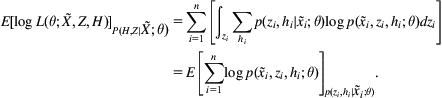
Here, ![]() means that an expectation is performed under the posterior distribution over hidden variables:
means that an expectation is performed under the posterior distribution over hidden variables: ![]() .
.
It turns out that there is a close relationship between the log marginal likelihood and the expected log-likelihood: the derivative of the expected log-likelihood with respect to the parameters of the model equals the derivative of the log marginal likelihood. The following derivation, based on applying the chain rule from calculus and considering a single training example for simplicity, demonstrates why this is true:

The final expression is the expectation of the derivative of the log joint likelihood. This relationship is with respect to the derivative of the log marginal likelihood and the expected derivative of the log joint likelihood. However, it is also possible to establish a direct relationship between the log marginal and expected log joint probabilities. The variational analysis in Appendix A.2 shows that
where H[.] is the entropy.
As a consequence of this analysis, to perform learning in a probability model with hidden variables, the marginal likelihood can be optimized using gradient ascent by instead computing and following the gradient of the expected log-likelihood, assuming that the posterior distribution over hidden variables can be computed. This prompts a general approach to learning in a hidden variable model based on following the expected gradient. This can be decomposed into three steps: (1) a P-step, which computes the posterior over hidden variables; (2) an E-step, which computes the expectation of the gradient given the posterior; and (3) a G-step, which uses gradient-based optimization to maximize the objective function with respect to the parameters.
The Expectation Maximization Algorithm
Using the expected log joint probability as a key quantity for learning in a probability model with hidden variables is better known in the context of the celebrated “expectation maximization” or EM algorithm, which we encountered in “The expectation maximization algorithm for a mixture of Gaussians” section. We discuss the general EM formulation next. Section 9.6 gives a concrete example comparing and contrasting the expected gradient approach and the EM approach, using the probabilistic formulation of principal component analysis.
The EM algorithm follows the expected gradient approach. However, EM is often used with models in which the M-step can be computed in closed form—in other words, when exact parameter updates can be found by setting the derivative of the expected log-likelihood with respect to the parameters to 0. These updates often take the same form as the simple maximum likelihood estimates that one would use to compute the parameters of a distribution, and are essentially just modified forms of the equations used for observed data that involve averages weighted over the posterior distribution in place of observed counts.
The EM algorithm consists of two steps: (1) an E-step that computes the expectations used in the expected log-likelihood and (2) an M-step in which the objective is maximized—typically using a closed-form parameter update.
In the following, we assume that we have only discrete hidden variables H. The probability of the observed data ![]() can be maximized by maximizing the log-likelihood
can be maximized by maximizing the log-likelihood ![]() of the parameters
of the parameters ![]() arising from an underlying latent variable model
arising from an underlying latent variable model ![]() as follows. Initialize the parameters as
as follows. Initialize the parameters as ![]() and repeat the following steps, where convergence is measured in terms of either the change to the log-likelihood or the degree of change to the parameters:
and repeat the following steps, where convergence is measured in terms of either the change to the log-likelihood or the degree of change to the parameters:
1. E-step: Compute required expectations involving ![]()
3. If the algorithm has not converged, set ![]() and return to step 1.
and return to step 1.
Note that the M-step corresponds to maximizing the expected log-likelihood. Although discrete hidden variables are used above, the approach generalizes to continuous ones.
For many latent variable models—Gaussian mixture models, PPCA, and hidden Markov models—the required posterior distributions can be computed exactly, which accounts for their popularity. However, for many other probabilistic models it is simply not possible to compute an exact posterior distribution. This can easily happen with multiple hidden random variables, because the posterior needed in the E-step is the joint posterior of the hidden variables. There is a vast literature on the subject of how to compute approximations to the true posterior distribution over hidden variables in more complex models.
Applying the Expectation Maximization Algorithm to Bayesian Networks
Bayesian networks capture statistical dependencies between attributes using an intuitive graphical structure, and the EM algorithm can easily be applied to such networks. Consider a Bayesian network with a number of discrete random variables, some of which are observed while others are not. Its marginal probability, in which hidden variables have been integrated out, can be maximized by maximizing the expected log joint probability over the posterior distribution of the hidden variables given the observed data—the expected log-likelihood.
For a network consisting of only discrete variables, this means that the E-step involves computing a distribution over hidden variables ![]() given observed variables
given observed variables ![]() or
or ![]() . If the network is a tree, this can be computed efficiently using the sum-product algorithm, which is explained in Section 9.6. If not, it can be computed efficiently using the junction tree algorithm. However, if the model is large, exact inference algorithms may be intractable, in which case a variational approximation or sampling procedure can be used to approximate the distribution.
. If the network is a tree, this can be computed efficiently using the sum-product algorithm, which is explained in Section 9.6. If not, it can be computed efficiently using the junction tree algorithm. However, if the model is large, exact inference algorithms may be intractable, in which case a variational approximation or sampling procedure can be used to approximate the distribution.
The M-step seeks
Recall that the log joint probability given by a Bayesian network decomposes into a sum over functions of subsets of variables. Notice also that the expression above involves an expectation using the joint conditional distribution or posterior over hidden variables. Using the EM algorithm, taking the derivative with respect to any given parameter leaves just terms that involve the marginal expectation over the distribution of variables that participate in the function for the gradient of the relevant parameter. This means, e.g., that to find the unconditional probability of an unobserved variable A in a network, it is necessary to determine the parameters ![]() of
of ![]() for which
for which
along with the further constraint that the probabilities in the discrete distribution sum to 1. This can be achieved using a Lagrange multiplier (Appendix A.2 gives an example of using this technique to estimate a discrete distribution). Setting the derivative of the constrained objective to 0 gives this closed form result:
In other words, the unconditional probability distribution is estimated in the same way in which it would be computed if the variables Ai had been observed, but with each observation replaced by its probability. Applying this procedure to the entire data set is tantamount to replacing observed counts with expected counts under the current model settings. If many examples have the same configuration, the distribution need only be computed once, and multiplied by the number of times that configuration has been seen.
Estimating entries in the network’s conditional probability tables also has an intuitive form. To estimate the conditional probability of unobserved random variable B given unobserved random variable A in a Bayesian network, simply compute their joint (posterior) probability and the marginal (posterior) probability of A for each example. Just as when the data is observed, the update equation is
This is just a ratio of the expected numbers of counts. If some of the variables are fully observed, the expression can be adapted by replacing the inferred probabilities by observed values—effectively assigning the observations a probability of 1. Furthermore, if variable B has multiple parents, A can be replaced by the set of parents.
9.5 Bayesian Estimation and Prediction
If there is reason to believe that a certain parameter has been drawn from a particular distribution, we can adopt a more Bayesian perspective. A common strategy is to employ a hyperparameter α to represent that distribution. Define the joint distribution of data and parameters as
Bayesian-style predictions use a quantity known as the posterior predictive distribution, which consists of the probability model for a new observation marginalized over the posterior probability inferred for the parameters given the observations so far. Again using a notation that explicitly differentiates variables ![]() from their observations
from their observations ![]() , the posterior predictive distribution is
, the posterior predictive distribution is
Given a Bayesian model that uses distributions over parameters, so-called “empirical Bayesian” methods can be employed to find a suitable value for the hyperparameter α. One such approach is obtained by maximizing the log marginal likelihood with respect to the model’s hyperparameters:
The remainder of this section demonstrates several techniques for creating complex structured probabilistic models.
Probabilistic Inference Methods
With complex probability models—and even with some seemingly simple ones—computing quantities such as posterior distributions, marginal distributions, and the maximum probability configuration, often require specialized methods to achieve results efficiently—even approximate ones. This is the field of probabilistic inference. Below we review some widely used probabilistic inference methods, including probability propagation, sampling and simulated annealing, and variational inference.
Probability propagation
Structured probability models like the Bayesian networks and Markov random fields discussed in Section 9.6 decompose a joint probability distribution into a factorized structure consisting of products of functions over subsets of variables. Then the task of computing marginal probabilities to find a maximum-probability configuration can be computationally demanding using brute force computation. In some cases even a naïve approach is completely infeasible in practice. However, it is sometimes possible to take advantage of the model’s structure to perform inference more efficiently. When Bayesian networks and related graphical models have an underlying tree connectivity structure, then belief propagation (also known as probability propagation) based on the sum-product and max-product algorithms presented in Section 9.6 can be applied to compute exact marginals, and hence the most probable model configuration.
Sampling, simulated annealing, and iterated conditional modes
With fully Bayesian methods that use distributions on parameters, or graphical models with cyclic structures, sampling methods are popular in both statistics and machine learning. Markov chain Monte Carlo methods are widely used to generate random samples from probability distributions that are difficult to compute. For example, as we have seen above, posterior distributions are often needed for expectations required during learning, but in many settings these can be difficult to compute. Gibbs sampling is a popular special case of the more general Metropolis–Hastings algorithm that allows one to generate samples from a joint distribution even when the true distribution is a complex continuous function. These samples can then be used to approximate expectations of interest, and also to approximate marginal distributions of subsets of variables by simply ignoring parts pertaining to other variables.
Gibbs sampling is conceptually very simple. Assign an initial set of states to the random variables of interest. With n random variables, this initial assignment or set of samples can be written ![]() . We then iteratively update each variable by sampling from its conditional distribution given the others:
. We then iteratively update each variable by sampling from its conditional distribution given the others:

In practice, these conditional distributions are often easy to compute. Furthermore, the idea of a “Markov blanket” introduced in Section 9.2 can often be used to reduce the number of variables necessary, because conditionals in structured models may depend on a much smaller subset of the variables.
To ensure an unbiased sample it is necessary to cycle through the data discarding samples in a process known as “burn-in.” The idea is to allow the Markov chain defined by the sampling procedure to approach its stationary distribution, and it can be shown that in the limit one will indeed obtain a sample from this distribution, and that the distribution corresponds to the underlying joint probability we wish to sample from. There is considerable theory concerning how much burn-in is required, but in practice it is common to discard samples arising from the first 100–1000 cycles. Sometimes, if more than one sample configuration is desired, averages are taken over k additional configurations of the sampler obtained after periods of about 100 cycles. We see how this procedure is used in practice in Section 9.6, under latent Dirichlet allocation.
Simulated annealing is a procedure that seeks an approximate most probable configuration or explanation. It adapts the Gibbs sampling procedure, described above, to include an iteration-dependent “temperature” term ti. Starting with an initial assignment ![]() , subsequent samples take the form
, subsequent samples take the form
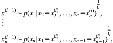
Where the temperature is decreased at each iteration: ti+1 < ti. If the schedule is slow enough, this process will converge to the true global minimum. But therein lies the catch: the temperature may have to decrease very slowly. However, this is often possible, particularly with an efficient implementation of the sampler.
Another well-known algorithm is the iterated conditional modes procedure, consisting of iterations of the form

This can be very fast, but prone to local minima. It can be useful when constructing more interesting graphical models and optimizing them quickly in an analogous, greedy way.
Variational inference
Rather than sampling from a distribution that is difficult to manipulate, the distribution can be approximated by a simpler, more tractable, function. Suppose we have a probability model with a set H of hidden variables and a set X of observed variables. Let ![]() be the exact posterior distribution of the model and
be the exact posterior distribution of the model and ![]() be an approximation to it, where
be an approximation to it, where ![]() is a set of so-called “variational parameters.” Variational methods for probability models commonly involve defining a simple form for q that makes it easy to optimize
is a set of so-called “variational parameters.” Variational methods for probability models commonly involve defining a simple form for q that makes it easy to optimize ![]() in a way that brings q closer to p. The theory of variation EM optimizes latent variable models by maximizing a lower bound on the log marginal likelihood. This so-called “variational bound” is described in Appendix A.2, where we see how the EM algorithm can be viewed through a variational analysis. This allows one to create EM algorithms using either exact or approximate posterior distributions. While statisticians often prefer sampling methods to variational ones, variational methods are popular in machine learning because they can be faster—and can also be combined with sampling methods.
in a way that brings q closer to p. The theory of variation EM optimizes latent variable models by maximizing a lower bound on the log marginal likelihood. This so-called “variational bound” is described in Appendix A.2, where we see how the EM algorithm can be viewed through a variational analysis. This allows one to create EM algorithms using either exact or approximate posterior distributions. While statisticians often prefer sampling methods to variational ones, variational methods are popular in machine learning because they can be faster—and can also be combined with sampling methods.
9.6 Graphical Models and Factor Graphs
Bayesian networks give an intuitive picture of a probabilistic model that corresponds directly with how we have decided to decompose the joint probability of the random variables representing attributes into a product of conditional and unconditional probability distributions. Mixture models, such as the Gaussian mixture models of Section 9.3, are alternative ways of approximating joint distributions. This section shows how such models can be illustrated using Bayesian networks, and introduces a generalization of Bayesian networks, the so-called “plate notation,” that allows one to visualize the result of techniques that treat parameters as random quantities. A further generalization, “factor graphs,” can represent and visualize an even wider class of probabilistic graphical models. As before, we view attributes as random variables and instances as observations of them; we also represent things like the label of a cluster by a random variable in a graph.
Graphical Models and Plate Notation
Consider a simple two-cluster Gaussian mixture model. It can be illustrated in the form of a Bayesian network with a binary random variable C for the cluster membership and a continuous random variable x for the real-valued attribute. In the mixture model, the joint distribution P(C, x) is the product of the prior P(C) and the conditional probability distribution P(x|C). This structure is illustrated by the Bayesian network in Fig. 9.8A, where for each state of C a different Gaussian is used for the conditional distribution of the continuous variable x.

Multiple Bayesian networks can be used to visualize the underlying joint likelihood that results when parameter estimation is performed. The probability model for N observations x1=x1, x2=x2, and xN=xN can be conceptualized as N Bayesian networks, one for each variable xi observed or instantiated to the value xi. Fig. 9.8B illustrates this, using shaded nodes to indicate which random variables are observed.
A “plate” is simply a box around a Bayesian network that denotes a certain number of replications of it. The plate in Fig. 9.8C indicates i=1,…,N networks, each with an observed value for xi. Plate notation captures a model for the joint probability of the entire data with a simple picture.
Bayesian networks, and more complex models comprising plates of Bayesian networks, are known as generative models because the probabilistic definition of the model can be used to randomly generate data governed by the probability distribution that the model represents. Bayesian hierarchical modeling involves defining a hierarchy of levels for the parameters of a model and using the rules of probability arising from the application of Bayesian methods to infer the parameter values given observed data. These can be drawn with graphical models in which both random variables and parameters are treated as random quantities. The section on latent Dirichlet allocation below gives an example of this technique.
Probabilistic Principal Component Analysis
Principal component analysis can be viewed as the consequence of performing parameter estimation in a special type of linear Gaussian hidden variable model. This connects the traditional view of this standard technique, presented in Chapter 8, Data transformations, with the probabilistic formulation discussed here, and leads to more advanced methods based on Boltzmann machines and autoencoders that are introduced in Chapter 10, Deep learning. The probabilistic formulation also helps deal with missing values. The underlying idea is to represent data as being generated by a Gaussian distributed continuous hidden latent variable that is linearly transformed under a Gaussian model. As a result, the principal components of a given data set correspond to an underlying factorized covariance model for a corresponding multivariate Gaussian distribution model for the data. This factorized model becomes apparent when the hidden variables of the underlying latent variable model are integrated out.
More specifically, a set of hidden variables is used to represent the input data in a space of reduced dimensionality. Each dimension corresponds to an independent random variable drawn from a Gaussian distribution with zero mean and unit variance. Let x be a random variable corresponding to the d-dimensional vectors of observed data, and h be a k-dimensional vector of hidden random variables. k is typically smaller than d (but need not be). Then the underlying joint probability model has this linear Gaussian form:
where the zero vector 0 and identity matrix I denote the mean and covariance matrix for the Gaussian distribution used for p(h), and p(x|h) is Gaussian with mean Wh+μ and a diagonal covariance matrix D. (The expression for the mean is where the term “linear” in “linear Gaussian” comes from.) The mean μ is included as a parameter, but it would be zero if we first mean-centered the data. Fig. 9.9A shows a Bayesian network for PPCA; it reveals intuitions about the probabilistic interpretation of principal component analysis based on hidden variables that will help in understanding other models discussed later.

Probabilistic PCA is a form of generative model, and Fig. 9.9A visualizes the associated underlying generative process. Data is generated by sampling each dimension of h from an independent Gaussian distribution and using the matrix Wh+μ to project this lower dimensional representation of the data into the observed, higher dimensional representation. Noise, specified by the diagonal covariance matrix D, is added separately to each dimension of the higher dimensional representation.
If the noise associated with the conditional distribution of x given h is the same in each dimension (i.e., isotropic) and infinitesimally small (such that ![]() ), a set of estimation equations can be derived that give the same principal components as those obtained by conventional principal component analysis. Restricting the covariance matrix D to be diagonal produces a model known as factor analysis). If D is isotropic (i.e., has the form
), a set of estimation equations can be derived that give the same principal components as those obtained by conventional principal component analysis. Restricting the covariance matrix D to be diagonal produces a model known as factor analysis). If D is isotropic (i.e., has the form ![]() ), then after optimizing the model and learning σ2 the columns of W will be scaled and rotated principal eigenvectors of the covariance matrix of the data. The contours of equal probability for a multivariate Gaussian distribution can be drawn with an ellipse whose principal axis corresponds to the principal eigenvector of the covariance matrix, as illustrated in Fig. 9.9B.
), then after optimizing the model and learning σ2 the columns of W will be scaled and rotated principal eigenvectors of the covariance matrix of the data. The contours of equal probability for a multivariate Gaussian distribution can be drawn with an ellipse whose principal axis corresponds to the principal eigenvector of the covariance matrix, as illustrated in Fig. 9.9B.
Because of the nice properties of Gaussian distributions, the marginal distributions of x in these models are also Gaussian, with parameters that can be computed analytically using simple algebraic expressions. For example, a model with ![]() has
has ![]() , which is the marginal distribution of x under the joint probability model, obtained by integrating out the uncertainty associated with h from the joint distribution p(x,h) defined earlier. Integrating out the hidden variables h from a PPCA model defines a Gaussian distribution whose covariance matrix M has the special form WWT+D. Appendix A.2 relates this factorization to an eigenvector analysis of the covariance matrix, resulting in the standard matrix factorization view of principal component analysis.
, which is the marginal distribution of x under the joint probability model, obtained by integrating out the uncertainty associated with h from the joint distribution p(x,h) defined earlier. Integrating out the hidden variables h from a PPCA model defines a Gaussian distribution whose covariance matrix M has the special form WWT+D. Appendix A.2 relates this factorization to an eigenvector analysis of the covariance matrix, resulting in the standard matrix factorization view of principal component analysis.
Inference with PPCA
As a result of the underlying linear Gaussian formulation, various other quantities needed for making inferences and performing parameter estimation can also be obtained analytically. For example, given ![]() , the posterior distribution for h can be obtained from Bayes’ rule, along with some Gaussian identities given in Appendix A.2. The posterior can be written
, the posterior distribution for h can be obtained from Bayes’ rule, along with some Gaussian identities given in Appendix A.2. The posterior can be written
(9.1)