
Wellbore Flow Performance
Abstract
Wellbore performance analysis involves establishing a relationship among tubular size, wellhead and bottom-hole pressure, fluid properties, and fluid production rate. Understanding wellbore flow performance is vitally important to production engineers for designing oil well equipment and optimizing well production conditions. Oil can be produced through tubing, casing, or both in an oil well, depending on which flow path provides better performance. Producing oil through tubing is a better option in most cases to take the advantage of gas-lift effects. The mathematical models are also valid for casing flow and casing-tubing annular flow as long as hydraulic diameter is used. Among many models, the modified Hagedorn–Brown model has been found to give results with good accuracy. The industry practice is to conduct a flow gradient (FG) survey to measure the flowing pressures along the tubing string. The FG data are then employed to validate one of the models and tune the model if necessary before the model is used on a large scale.
Keywords
TPR; VLP; wellbore; flow; hydraulics
4.1 Introduction
Chapter 3, Reservoir Deliverability described reservoir deliverability. However, the achievable oil production rate from a well is determined by wellhead pressure and the flow performance of production string; that is, tubing, casing, or both. The flow performance of production string depends on geometries of the production string and properties of fluids being produced. The fluids in oil wells include oil, water, gas, and sand. Wellbore performance analysis involves establishing a relationship between tubular size, wellhead and bottom-hole pressure, fluid properties, and fluid production rate. Understanding wellbore flow performance is vitally important to production engineers for designing oil well equipment and optimizing well production conditions.
Oil can be produced through tubing, casing, or both in an oil well, depending on which flow path has better performance. Producing oil through ubing is a better option in most cases to take the advantage of gas-lift effect. The traditional term tubing performance relationship (TPR) is used in this book (other terms such as vertical lift performance have been used in the literature). However, the mathematical models are also valid for casing flow and casing-tubing annular flow as long as hydraulic diameter is used. This chapter focuses on determination of TPR and pressure traverse along the well string. Both single-phase and multiphase fluids are considered. Calculation examples are illustrated with hand calculations and computer spreadsheets that are provided with this book.
4.2 Single-Phase Liquid Flow
Single-phase liquid flow exists in an oil well only when the wellhead pressure is above the bubble-point pressure of the oil, which is usually not a reality. However, it is convenient to start from single-phase liquid for establishing the concept of fluid flow in oil wells where multiphase flow usually dominates.
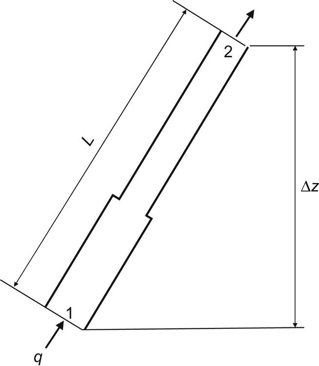
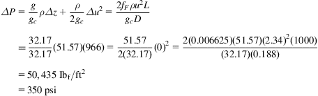
Consider a fluid flowing from point 1 to point 2 in a tubing string of length L and height Δz (Fig. 4.1). The first law of thermodynamics yields the following equation for pressure drop:
(4.1)
P1=pressure at point 1, lbf/ft2
P2=pressure at point 2, lbf/ft2
g=gravitational acceleration, 32.17 ft/s2
The first, second, and third terms in the right-hand side of the equation represent pressure drops due to changes in elevation, kinetic energy, and friction, respectively.
The Fanning friction factor (fF) can be evaluated based on Reynolds number and relative roughness. Reynolds number is defined as the ratio of inertial force to viscous force. The Reynolds number is expressed in consistent units as
(4.2)
or in U.S. field units as
(4.3)
For laminar flow where NRe<2000, the fF is inversely proportional to the Reynolds number, or
(4.4)
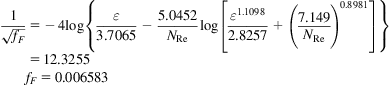
For turbulent flow where NRe>2100, the fF can be estimated using empirical correlations. Among numerous correlations developed by different investigators, Chen’s (1979) correlation has an explicit form and gives similar accuracy to the Colebrook–White equation (Gregory and Fogarasi, 1985) that was used for generating the friction factor chart used in the petroleum industry. Chen’s correlation takes the following form:
(4.5)
where the relative roughness is defined as ![]() , and δ is the absolute roughness of pipe wall.
, and δ is the absolute roughness of pipe wall.
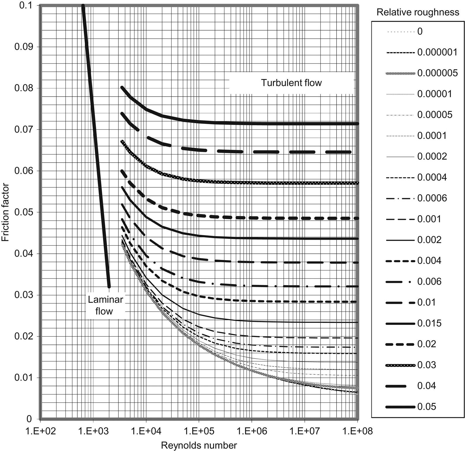
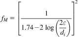
The fF can also be obtained based on Darcy–Wiesbach friction factor shown in Fig. 4.2. The Darcy–Wiesbach friction factor is also referred to as the Moody friction factor (fM) in some literatures. The relation between the Moody and the fF is expressed as
(4.6)
Example Problem 4.1 Suppose that 1000 bbl/day of 40 °API, 1.2 cp oil is being produced through ![]() -in., 8.6-lbm/ft tubing in a well that is 15° from vertical. If the tubing wall relative roughness is 0.001, calculate the pressure drop over 1000 ft of tubing.
-in., 8.6-lbm/ft tubing in a well that is 15° from vertical. If the tubing wall relative roughness is 0.001, calculate the pressure drop over 1000 ft of tubing.
Solution Oil-specific gravity:
Oil density:
Elevation increase:
The ![]() -in., 8.6-lbm/ft tubing has an inner diameter of 2.259 in. Therefore,
-in., 8.6-lbm/ft tubing has an inner diameter of 2.259 in. Therefore,

Fluid velocity can be calculated accordingly:
Reynolds number:
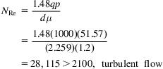
Chen’s correlation gives
If Fig. 4.2 is used, the chart gives a fM of 0.0265. Thus, the fF is estimated as

Finally, the pressure drop is calculated:
4.3 Single-Phase Gas Flow
The first law of thermodynamics (conservation of energy) governs gas flow in tubing. The effect of kinetic energy change is negligible because the variation in tubing diameter is insignificant in most gas wells. With no shaft work device installed along the tubing string, the first law of thermodynamics yields the following mechanical balance equation:
(4.7)
Because dZ=cos θdL, ![]() , and
, and ![]() Eq. (4.7) can be rewritten as
Eq. (4.7) can be rewritten as
(4.8)
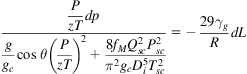
which is an ordinary differential equation governing gas flow in tubing. Although the temperature T can be approximately expressed as a linear function of length L through geothermal gradient, the compressibility factor z is a function of pressure P and temperature T. This makes it difficult to solve the equation analytically. Fortunately, the pressure P at length L is not a strong function of temperature and compressibility factor. Approximate solutions to Eq. (4.8) have been sought and used in the natural gas industry.
4.3.1 Average Temperature and Compressibility Factor Method
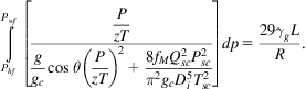
If single average values of temperature and compressibility factor over the entire tubing length can be assumed, Eq. (4.8) becomes
(4.9)
By separation of variables, Eq. (4.9) can be integrated over the full length of tubing to yield
(4.10)
where
(4.11)
Eqs. (4.10) and (4.11) take the following forms when U.S. field units (qsc in Mscf/d), are used (Katz et al., 1959):
(4.12)
and
(4.13)
The Darcy–Wiesbach (Moody) friction factor fM can be found in the conventional manner for a given tubing diameter, wall roughness, and Reynolds number. However, if one assumes fully turbulent flow, which is the case for most gas wells, then a simple empirical relation may be used for typical tubing strings (Katz and Lee, 1990):
(4.14)
(4.15)
Guo and Ghalambor (2002) used the following Nikuradse friction factor correlation for fully turbulent flow in rough pipes:
(4.16)
 (4.16)
Because the average compressibility factor is a function of pressure itself, a numerical technique such as Newton–Raphson iteration is required to solve Eq. (4.12) for bottom-hole pressure. This computation can be performed automatically with the spreadsheet program Average TZ.xls. Users need to input parameter values in the Input data section and run Macro Solution to get results.
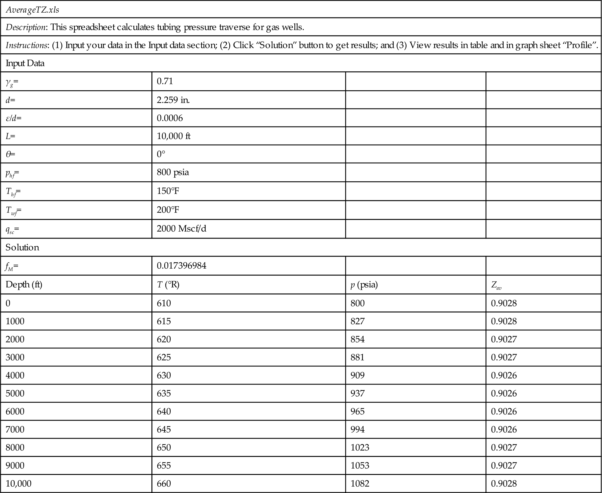
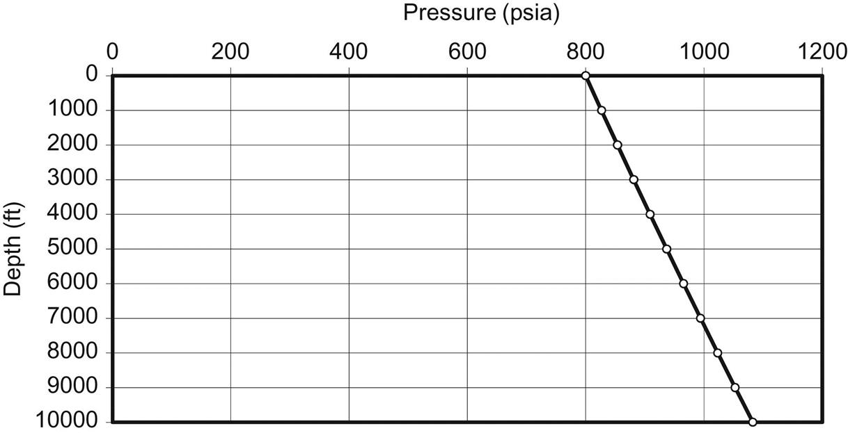
Example Problem 4.2 Suppose that a vertical well produces 2 MMscf/d of 0.71 gas-specific gravity gas through a ![]() in. tubing set to the top of a gas reservoir at a depth of 10,000 ft. At tubing head, the pressure is 800 psia and the temperature is 150°F; the bottom-hole temperature is 200°F. The relative roughness of tubing is about 0.0006. Calculate the pressure profile along the tubing length and plot the results.
in. tubing set to the top of a gas reservoir at a depth of 10,000 ft. At tubing head, the pressure is 800 psia and the temperature is 150°F; the bottom-hole temperature is 200°F. The relative roughness of tubing is about 0.0006. Calculate the pressure profile along the tubing length and plot the results.
Solution Example Problem 4.2 is solved with the spreadsheet program AverageTZ.xls. Table 4.1 shows the appearance of the spreadsheet for the Input data and Result sections. The calculated pressure profile is plotted in Fig. 4.3.
Table 4.1
Spreadsheet AverageTZ.xls: The Input Data and Result Sections
| AverageTZ.xls | |||
| Description: This spreadsheet calculates tubing pressure traverse for gas wells. | |||
| Instructions: (1) Input your data in the Input data section; (2) Click “Solution” button to get results; and (3) View results in table and in graph sheet “Profile”. | |||
| Input Data | |||
| γg= | 0.71 | ||
| d= | 2.259 in. | ||
| ε/d= | 0.0006 | ||
| L= | 10,000 ft | ||
| θ= | 0° | ||
| phf= | 800 psia | ||
| Thf= | 150°F | ||
| Twf= | 200°F | ||
| qsc= | 2000 Mscf/d | ||
| Solution | |||
| fM= | 0.017396984 | ||
| Depth (ft) | T (°R) | p (psia) | Zav |
| 0 | 610 | 800 | 0.9028 |
| 1000 | 615 | 827 | 0.9028 |
| 2000 | 620 | 854 | 0.9027 |
| 3000 | 625 | 881 | 0.9027 |
| 4000 | 630 | 909 | 0.9026 |
| 5000 | 635 | 937 | 0.9026 |
| 6000 | 640 | 965 | 0.9026 |
| 7000 | 645 | 994 | 0.9026 |
| 8000 | 650 | 1023 | 0.9027 |
| 9000 | 655 | 1053 | 0.9027 |
| 10,000 | 660 | 1082 | 0.9028 |
4.3.2 Cullender and Smith Method
Eq. (4.8) can be solved for bottom-hole pressure using a fast numerical algorithm originally developed by Cullender and Smith (Katz et al., 1959). Eq. (4.8) can be rearranged as
(4.17)
 (4.17)
that takes an integration form of
(4.18)
 (4.18)
In U.S. field units (qmsc in MMscf/d), Eq. (4.18) has the following form:
(4.19)
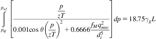 (4.19)
If the integrant is denoted with symbol I, that is,
(4.20)
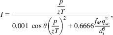 (4.20)
Eq. (4.19) becomes
(4.21)
In the form of numerical integration, Eq. (4.21) can be expressed as
(4.22)
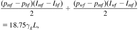 (4.22)
where pmf is the pressure at the mid-depth. The Ihf, Imf, and Iwf are integrant is evaluated at phf, pmf, and pwf, respectively. Assuming the first and second terms in the right-hand side of Eq. (4.22) each represents half of the integration, that is,
(4.23)
(4.24)
the following expressions are obtained:
(4.25)
(4.26)
Because Imf is a function of pressure pmf itself, a numerical technique such as Newton–Raphson iteration is required to solve Eq. (4.25) for pmf. Once pmf is computed, pwf can be solved numerically from Eq. (4.26). These computations can be performed automatically with the spreadsheet program Cullender-Smith.xls. Users need to input parameter values in the Input Data section and run Macro Solution to get results.
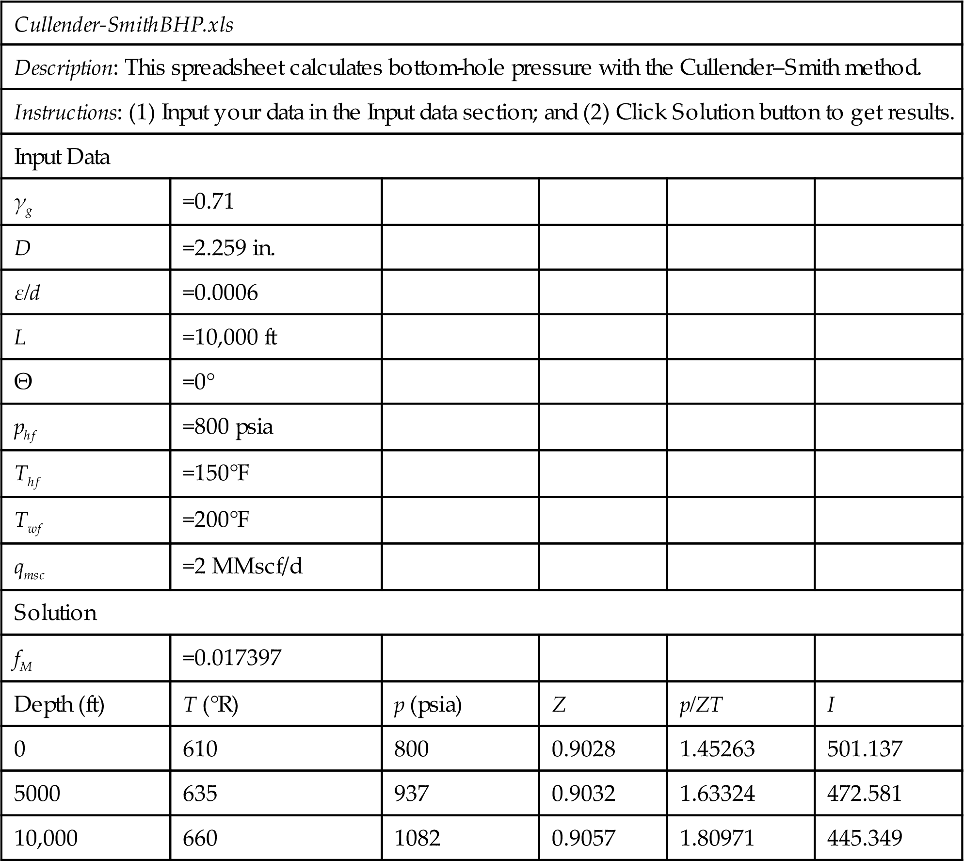
Example Problem 4.3 Solve the problem in Example Problem 4.2 with the Cullender and Smith Method.
Solution Example Problem 4.3 is solved with the spreadsheet program Cullender-Smith.xls. Table 4.2 shows the appearance of the spreadsheet for the Input data and Result sections. The pressures at depths of 5000 ft and 10,000 ft are 937 psia and 1082 psia, respectively. These results are exactly the same as that given by the Average Temperature and Compressibility Factor Method.
Table 4.2
Spreadsheet Cullender-Smith.xls: The Input Data and Result Sections
| Cullender-SmithBHP.xls | |||||
| Description: This spreadsheet calculates bottom-hole pressure with the Cullender–Smith method. | |||||
| Instructions: (1) Input your data in the Input data section; and (2) Click Solution button to get results. | |||||
| Input Data | |||||
| γg | =0.71 | ||||
| D | =2.259 in. | ||||
| ε/d | =0.0006 | ||||
| L | =10,000 ft | ||||
| Θ | =0° | ||||
| phf | =800 psia | ||||
| Thf | =150°F | ||||
| Twf | =200°F | ||||
| qmsc | =2 MMscf/d | ||||
| Solution | |||||
| fM | =0.017397 | ||||
| Depth (ft) | T (°R) | p (psia) | Z | p/ZT | I |
| 0 | 610 | 800 | 0.9028 | 1.45263 | 501.137 |
| 5000 | 635 | 937 | 0.9032 | 1.63324 | 472.581 |
| 10,000 | 660 | 1082 | 0.9057 | 1.80971 | 445.349 |
4.3.3 Flow of Impure Gas
The average temperature average z-factor method and the Cullender and Smith method were derived on the basis of pure gas flow. In reality, almost all gas wells produce certain amount of liquids (oil and water) and sometimes solid particles (sand and coal). The volume fractions of these liquids and solids are low but their effect on pressure can be significant due to their densities being much higher than the density of gas.
A gas-oil-water-sand four-phase flow model was proposed by Guo and Ghalambor (2005) to describe the flow impure gas. The model takes a closed (integrated) form, which makes it easy to use. The Guo–Ghalambor model can be expressed as follows:
(4.27)
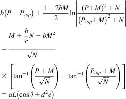 (4.27)
where the group parameters are defined as
(4.28)
(4.29)
(4.30)
(4.31)
(4.32)
(4.33)
(4.34)
A=cross-sectional area of conduit, in.2
fM=Darcy–Wiesbach friction factor (Moody factor)
g=gravitational acceleration, 32.17 ft/s2
Ptop=flowing pressure at section top, lbf/ft2
qs=sand production rate, ft3/day
qw=water production rate, bbl/d
γg=specific gravity of gas, air=1
γo=specific gravity of produced oil, freshwater=1
The Darcy–Wiesbach friction factor (fM) can be obtained from diagram (Fig. 4.2) or based on fF obtained from Eq. (4.16). The required relation is fM=4fF. The Guo–Ghalambor can also be used for describing mist flow in oil wells (Guo et al., 2008).
Because iterations are required to solve Eq. (4.18) for pressure, a computer spreadsheet program Guo-Ghalambor BHP.xls has been developed.
Example Problem 4.4 For the following data, estimate bottom-hole pressure with the Guo–Ghalambor method:
| Total measured depth: | 7000 ft |
| The average inclination angle: | 20° |
| Tubing inner diameter: | 1.995 in. |
| Gas production rate: | 1 MMscfd |
| Gas-specific gravity: | 0.7 air=1 |
| Oil production rate: | 1000 stb/d |
| Oil-specific gravity: | 0.85 H2O=1 |
| Water production rate: | 300 bbl/d |
| Water-specific gravity: | 1.05 H2O=1 |
| Solid production rate: | 1 ft3/d |
| Solid-specific gravity: | 2.65 H2O=1 |
| Tubing head temperature: | 100°F |
| Bottom-hole temperature: | 224°F |
| Tubing head pressure: | 300 psia |
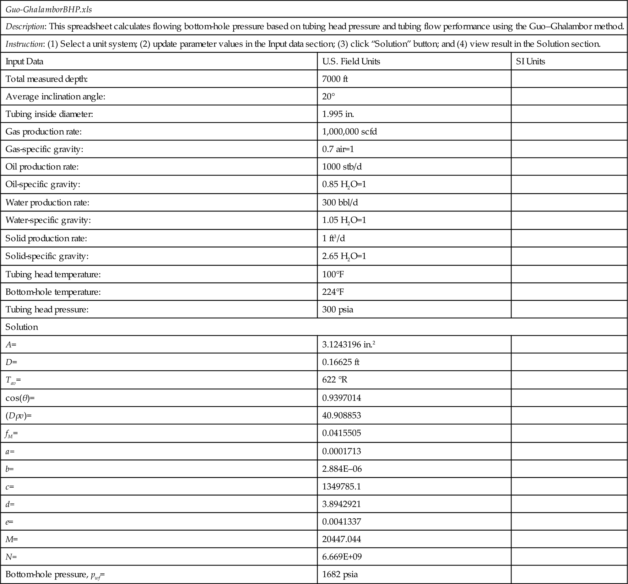
Solution This example problem is solved with the spreadsheet program Guo-GhalamborBHP.xls. The result is shown in Table 4.2. and Table 4.3.
Table 4.3
Result Given by Guo-GhalamborBHP.xls for Example Problem 4.3
| Guo-GhalamborBHP.xls | ||
| Description: This spreadsheet calculates flowing bottom-hole pressure based on tubing head pressure and tubing flow performance using the Guo–Ghalambor method. | ||
| Instruction: (1) Select a unit system; (2) update parameter values in the Input data section; (3) click “Solution” button; and (4) view result in the Solution section. | ||
| Input Data | U.S. Field Units | SI Units |
| Total measured depth: | 7000 ft | |
| Average inclination angle: | 20° | |
| Tubing inside diameter: | 1.995 in. | |
| Gas production rate: | 1,000,000 scfd | |
| Gas-specific gravity: | 0.7 air=1 | |
| Oil production rate: | 1000 stb/d | |
| Oil-specific gravity: | 0.85 H2O=1 | |
| Water production rate: | 300 bbl/d | |
| Water-specific gravity: | 1.05 H2O=1 | |
| Solid production rate: | 1 ft3/d | |
| Solid-specific gravity: | 2.65 H2O=1 | |
| Tubing head temperature: | 100°F | |
| Bottom-hole temperature: | 224°F | |
| Tubing head pressure: | 300 psia | |
| Solution | ||
| A= | 3.1243196 in.2 | |
| D= | 0.16625 ft | |
| Tav= | 622 °R | |
| cos(θ)= | 0.9397014 | |
| (Dρv)= | 40.908853 | |
| fM= | 0.0415505 | |
| a= | 0.0001713 | |
| b= | 2.884E–06 | |
| c= | 1349785.1 | |
| d= | 3.8942921 | |
| e= | 0.0041337 | |
| M= | 20447.044 | |
| N= | 6.669E+09 | |
| Bottom-hole pressure, pwf= | 1682 psia | |
4.4 Multiphase Flow in Oil Wells
In addition to oil, almost all oil wells produce a certain amount of water, gas, and sometimes sand. These wells are called multiphase oil wells. The TPR equation for single-phase flow is not valid for multiphase oil wells. To analyze TPR of multiphase oil wells rigorously, a multiphase flow model is required.
Multiphase flow is much more complicated than single-phase flow because of the variation of flow regime (or flow pattern). Fluid distribution changes greatly in different flow regimes, which significantly affects pressure gradient in the tubing.
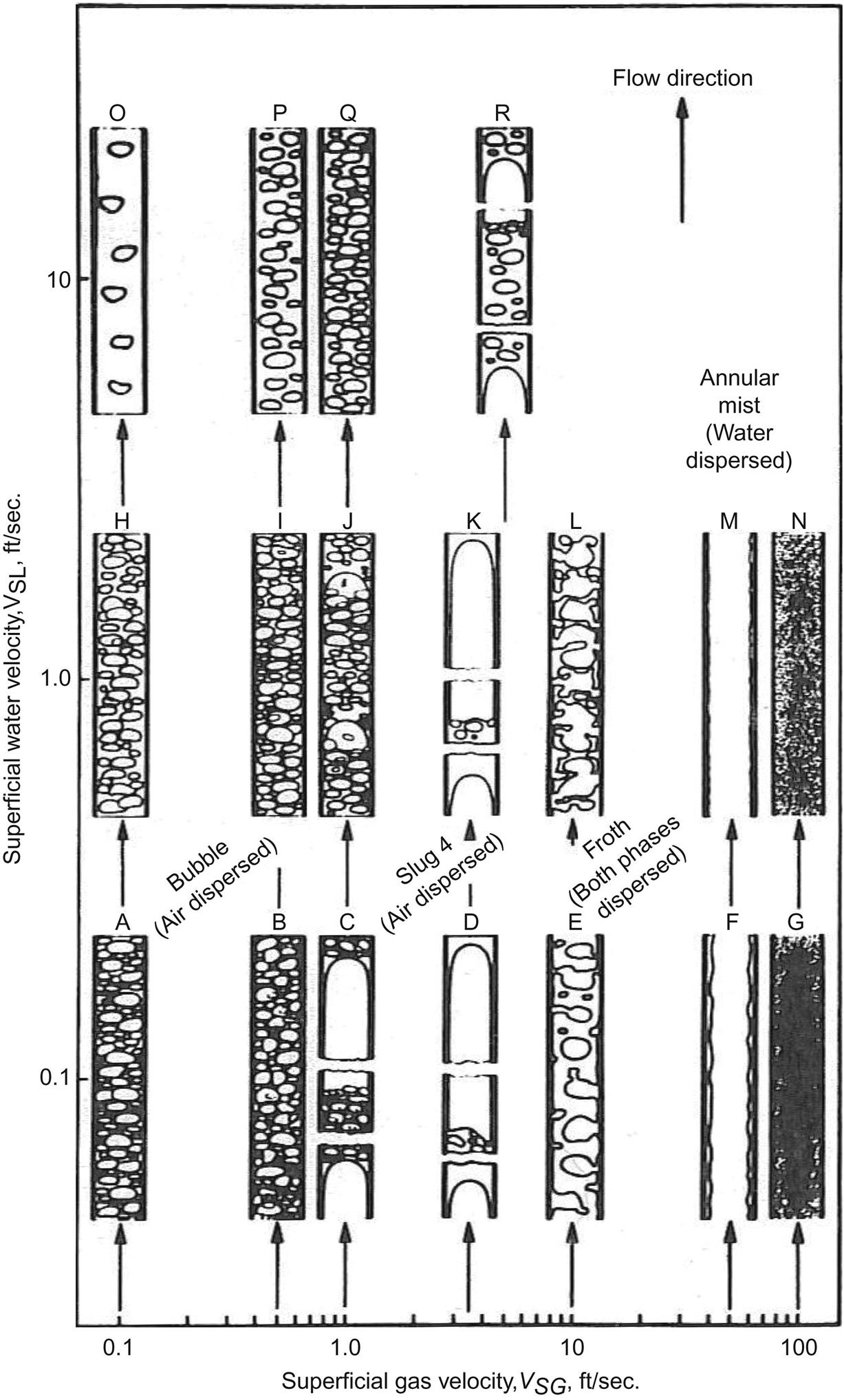
4.4.1 Flow Regimes
As shown in Fig. 4.4, at least four flow regimes have been identified in gas-liquid two-phase flow. They are bubble, slug, churn, and annular flow. These flow regimes occur as a progression with increasing gas flow rate for a given liquid flow rate. In bubble flow, gas phase is dispersed in the form of small bubbles in a continuous liquid phase. In slug flow, gas bubbles coalesce into larger bubbles that eventually fill the entire pipe cross-section. Between the large bubbles are slugs of liquid that contain smaller bubbles of entrained gas. In churn flow, the larger gas bubbles become unstable and collapse, resulting in a highly turbulent flow pattern with both phases dispersed. In annular flow, gas becomes the continuous phase, with liquid flowing in an annulus, coating the surface of the pipe and with droplets entrained in the gas phase.
4.4.2 Liquid Holdup
In multiphase flow, the amount of the pipe occupied by a phase is often different from its proportion of the total volumetric flow rate. This is due to density difference between phases. The density difference causes dense phase to slip down in an upward flow (i.e., the lighter phase moves faster than the denser phase). Because of this, the in-situ volume fraction of the denser phase will be greater than the input volume fraction of the denser phase (i.e., the denser phase is “held up” in the pipe relative to the lighter phase). Thus, liquid “holdup” is defined as
(4.35)
Liquid holdup depends on flow regime, fluid properties, and pipe size and configuration. Its value can be quantitatively determined only through experimental measurements.
4.4.3 TPR Models
Numerous TPR models have been developed for analyzing multiphase flow in vertical pipes. Brown (1977) presents a thorough review of these models. TPR models for multiphase flow wells fall into two categories: (1) homogeneous-flow models and (2) separated-flow models. Homogeneous models treat multiphase as a homogeneous mixture and do not consider the effects of liquid holdup (no-slip assumption). Therefore, these models are less accurate and are usually calibrated with local operating conditions in field applications. The major advantage of these models comes from their mechanistic nature. They can handle gas-oil-water three-phase and gas-oil-water-sand four-phase systems. It is easy to code these mechanistic models in computer programs.
Separated-flow models are more realistic than the homogeneous-flow models. They are usually given in the form of empirical correlations. The effects of liquid holdup (slip) and flow regime are considered. The major disadvantage of the separated-flow models is that it is difficult to code them in computer programs because most correlations are presented in graphic form.
4.4.3.1 Homogeneous-flow models
Numerous homogeneous-flow models have been developed for analyzing the TPR of multiphase wells since the pioneering works of Poettmann and Carpenter (1952). Poettmann–Carpenter’s model uses empirical two-phase friction factor for friction pressure loss calculations without considering the effect of liquid viscosity. The effect of liquid viscosity was considered by later researchers including Cicchitti (1960) and Dukler et al. (1964). A comprehensive review of these models was given by Hasan and Kabir (2002). Guo and Ghalambor (2005) presented work addressing gas-oil-water-sand four-phase flow.
Assuming no slip of liquid phase, Poettmann and Carpenter (1952) presented a simplified gas-oil-water three-phase flow model to compute pressure losses in wellbores by estimating mixture density and friction factor. According to Poettmann and Carpenter, the following equation can be used to calculate pressure traverse in a vertical tubing when the acceleration term is neglected:
(4.36)
and
(4.37)
f2F=Fanning friction factor for two-phase flow
qo=oil production rate, stb/day
The average mixture density ![]() can be calculated by
can be calculated by
(4.38)
The mixture density at a given point can be calculated based on mass flow rate and volume flow rate:
(4.39)
where
(4.40)
(4.41)
γo=oil-specific gravity, 1 for freshwater
WOR=producing water–oil ratio, bbl/stb
γw=water-specific gravity, 1 for freshwater
GOR=producing gas–oil ratio, scf/stb
γg=gas-specific gravity, 1 for air
Vm=volume of mixture associated with 1 stb of oil, ft3
Bo=formation volume factor of oil, rb/stb
Bw=formation volume factor of water, rb/bbl
If data from direct measurements are not available, solution gas–oil ratio and formation volume factor of oil can be estimated using the following correlations:
(4.42)
(4.43)
where t is in-situ temperature in °F. The two-phase friction factor f2F can be estimated from a chart recommended by Poettmann and Carpenter (1952). For easy coding in computer programs, Guo and Ghalambor (2002) developed the following correlation to represent the chart:
(4.44)
where (Dρv) is the numerator of Reynolds number representing inertial force and can be formulated as
(4.45)
Because the Poettmann–Carpenter model takes a finite-difference form, this model is accurate for only short-depth incremental Δh. For deep wells, this model should be used in a piecewise manner to get accurate results (i.e., the tubing string should be “broken” into small segments and the model is applied to each segment).
Because iterations are required to solve Eq. (4.36) for pressure, a computer spreadsheet program Poettmann-CarpenterBHP.xls has been developed. The program is available from the attached CD.
Example Problem 4.5 For the following given data, calculate bottom-hole pressure:
| Tubing head pressure: | 500 psia |
| Tubing head temperature: | 100°F |
| Tubing inner diameter: | 1.66 in. |
| Tubing shoe depth (near bottom hole): | 5000 ft |
| Bottom-hole temperature: | 150°F |
| Liquid production rate: | 2000 stb/day |
| Water cut: | 25% |
| Producing GLR: | 1000 scf/stb |
| Oil gravity: | 30 °API |
| Water-specific gravity: | 1.05 1 for freshwater |
| Gas-specific gravity: | 0.65 1 for air |
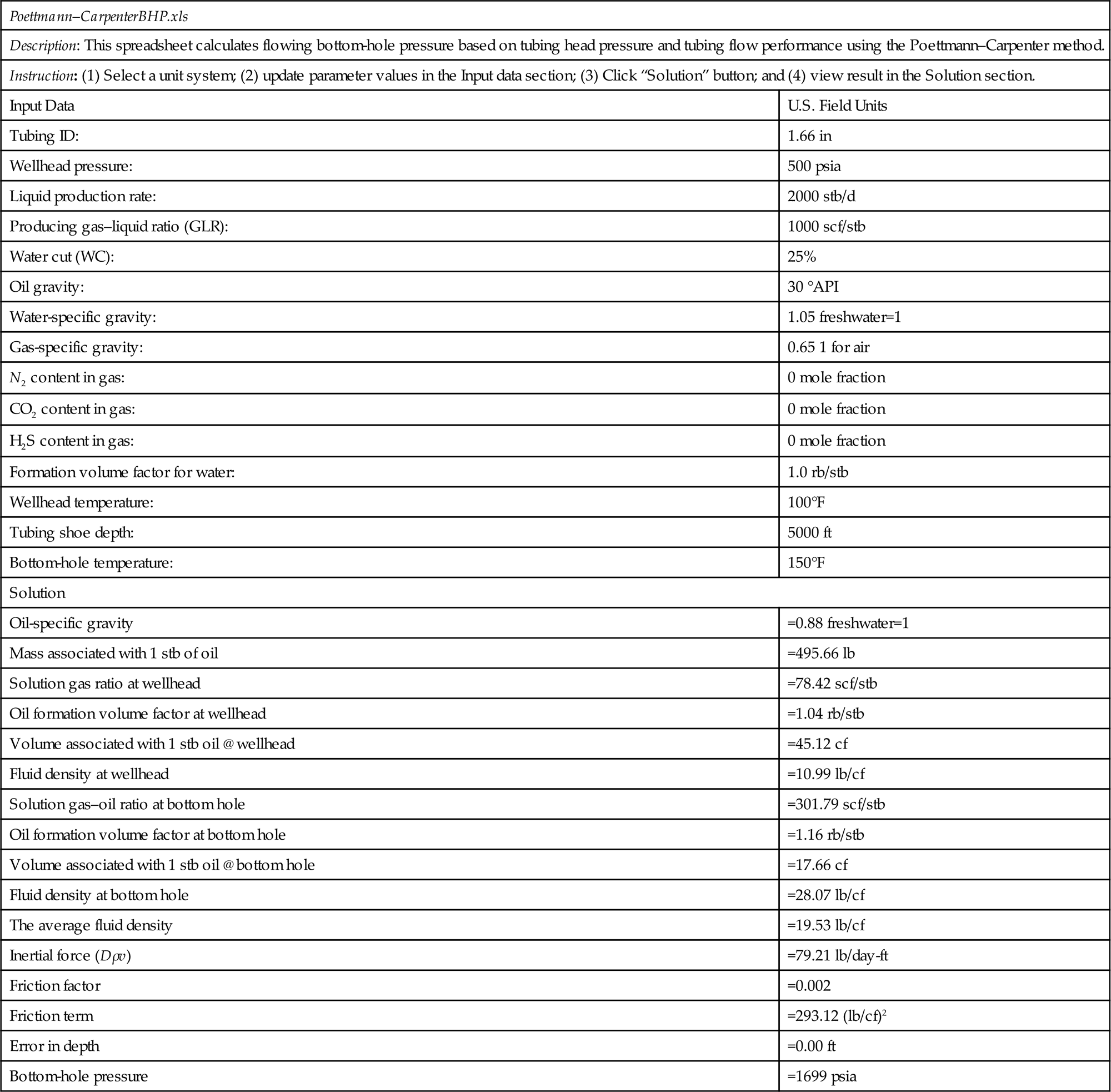
Solution This problem can be solved using the computer program Poettmann-CarpenterBHP.xls. The result is shown in Table 4.4.
Table 4.4
Result Given by Poettmann-CarpenterBHP.xls for Example Problem 4.2
| Poettmann–CarpenterBHP.xls | |
| Description: This spreadsheet calculates flowing bottom-hole pressure based on tubing head pressure and tubing flow performance using the Poettmann–Carpenter method. | |
| Instruction: (1) Select a unit system; (2) update parameter values in the Input data section; (3) Click “Solution” button; and (4) view result in the Solution section. | |
| Input Data | U.S. Field Units |
| Tubing ID: | 1.66 in |
| Wellhead pressure: | 500 psia |
| Liquid production rate: | 2000 stb/d |
| Producing gas–liquid ratio (GLR): | 1000 scf/stb |
| Water cut (WC): | 25% |
| Oil gravity: | 30 °API |
| Water-specific gravity: | 1.05 freshwater=1 |
| Gas-specific gravity: | 0.65 1 for air |
| N2 content in gas: | 0 mole fraction |
| CO2 content in gas: | 0 mole fraction |
| H2S content in gas: | 0 mole fraction |
| Formation volume factor for water: | 1.0 rb/stb |
| Wellhead temperature: | 100°F |
| Tubing shoe depth: | 5000 ft |
| Bottom-hole temperature: | 150°F |
| Solution | |
| Oil-specific gravity | =0.88 freshwater=1 |
| Mass associated with 1 stb of oil | =495.66 lb |
| Solution gas ratio at wellhead | =78.42 scf/stb |
| Oil formation volume factor at wellhead | =1.04 rb/stb |
| Volume associated with 1 stb oil @ wellhead | =45.12 cf |
| Fluid density at wellhead | =10.99 lb/cf |
| Solution gas–oil ratio at bottom hole | =301.79 scf/stb |
| Oil formation volume factor at bottom hole | =1.16 rb/stb |
| Volume associated with 1 stb oil @ bottom hole | =17.66 cf |
| Fluid density at bottom hole | =28.07 lb/cf |
| The average fluid density | =19.53 lb/cf |
| Inertial force (Dρv) | =79.21 lb/day-ft |
| Friction factor | =0.002 |
| Friction term | =293.12 (lb/cf)2 |
| Error in depth | =0.00 ft |
| Bottom-hole pressure | =1699 psia |
4.4.3.2 Separated-flow models
A number of separated-flow models are available for TPR calculations. Among many others are the Lockhart and Martinelli correlation (1949), the Duns and Ros correlation (1963), and the Hagedorn and Brown method (1965). Based on comprehensive comparisons of these models, Ansari et al. (1994) and Hasan and Kabir (2002) recommended the Hagedorn–Brown method with modifications for near-vertical flow.
The modified Hagedorn–Brown (mH-B) method is an empirical correlation developed on the basis of the original work of Hagedorn and Brown (1965). The modifications include using the no-slip liquid holdup when the original correlation predicts a liquid holdup value less than the no-slip holdup and using the Griffith correlation (Griffith and Wallis, 1961) for the bubble flow regime.
The original Hagedorn–Brown correlation takes the following form:
(4.46)
which can be expressed in U.S. field units as
(4.47)
and
(4.48)
(4.49)
The superficial velocity of a given phase is defined as the volumetric flow rate of the phase divided by the pipe cross-sectional area for flow. The third term in the right-hand side of Eq. (4.47) represents pressure change due to kinetic energy change, which is in most instances negligible for oil wells.
Obviously, determination of the value of liquid holdup yL is essential for pressure calculations. The mH-B correlation uses liquid holdup from three charts using the following dimensionless numbers:
Liquid velocity number, NvL:
(4.50)
Gas velocity number, NvG:
(4.51)
Pipe diameter number, ND:
(4.52)
Liquid viscosity number, NL:
(4.53)
The first chart is used for determining parameter (CNL) based on NL. We have found that this chart can be replaced by the following correlation with acceptable accuracy:
(4.54)
where
(4.55)
and
(4.56)
Once the value of parameter (CNL) is determined, it is used for calculating the value of the group ![]() , where p is the absolute pressure at the location where pressure gradient is to be calculated, and pa is atmospheric pressure. The value of this group is then used as an entry in the second chart to determine parameter (yL/ψ). We have found that the second chart can be represented by the following correlation with good accuracy:
, where p is the absolute pressure at the location where pressure gradient is to be calculated, and pa is atmospheric pressure. The value of this group is then used as an entry in the second chart to determine parameter (yL/ψ). We have found that the second chart can be represented by the following correlation with good accuracy:
(4.57)
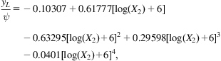 (4.57)
where
(4.58)
According to Hagedorn and Brown (1965), the value of parameter ψ can be determined from the third chart using a value of group ![]() .
.
We have found that for ![]() the third chart can be replaced by the following correlation with acceptable accuracy:
the third chart can be replaced by the following correlation with acceptable accuracy:
(4.59)
where
(4.60)
However, ψ=1.0 should be used for ![]() .
.
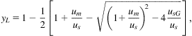
Finally, the liquid holdup can be calculated by
(4.61)
The Reynolds number for multiphase flow can be calculated by
(4.62)
where mt is mass flow rate. The modified mH-B method uses the Griffith correlation for the bubble-flow regime. The bubble-flow regime has been observed to exist when
(4.63)
where
(4.64)
and
(4.65)
which is valid for LB≥0.13. When the LB value given by Eq. (4.65) is less than 0.13, LB=0. 13 should be used.
Neglecting the kinetic energy pressure drop term, the Griffith correlation in U.S. field units can be expressed as
(4.66)
where mL is mass flow rate of liquid only. The liquid holdup in Griffith correlation is given by the following expression:
(4.67)
 (4.67)
where μs=0.8 ft/s. The Reynolds number used to obtain the friction factor is based on the in-situ average liquid velocity, that is,
(4.68)
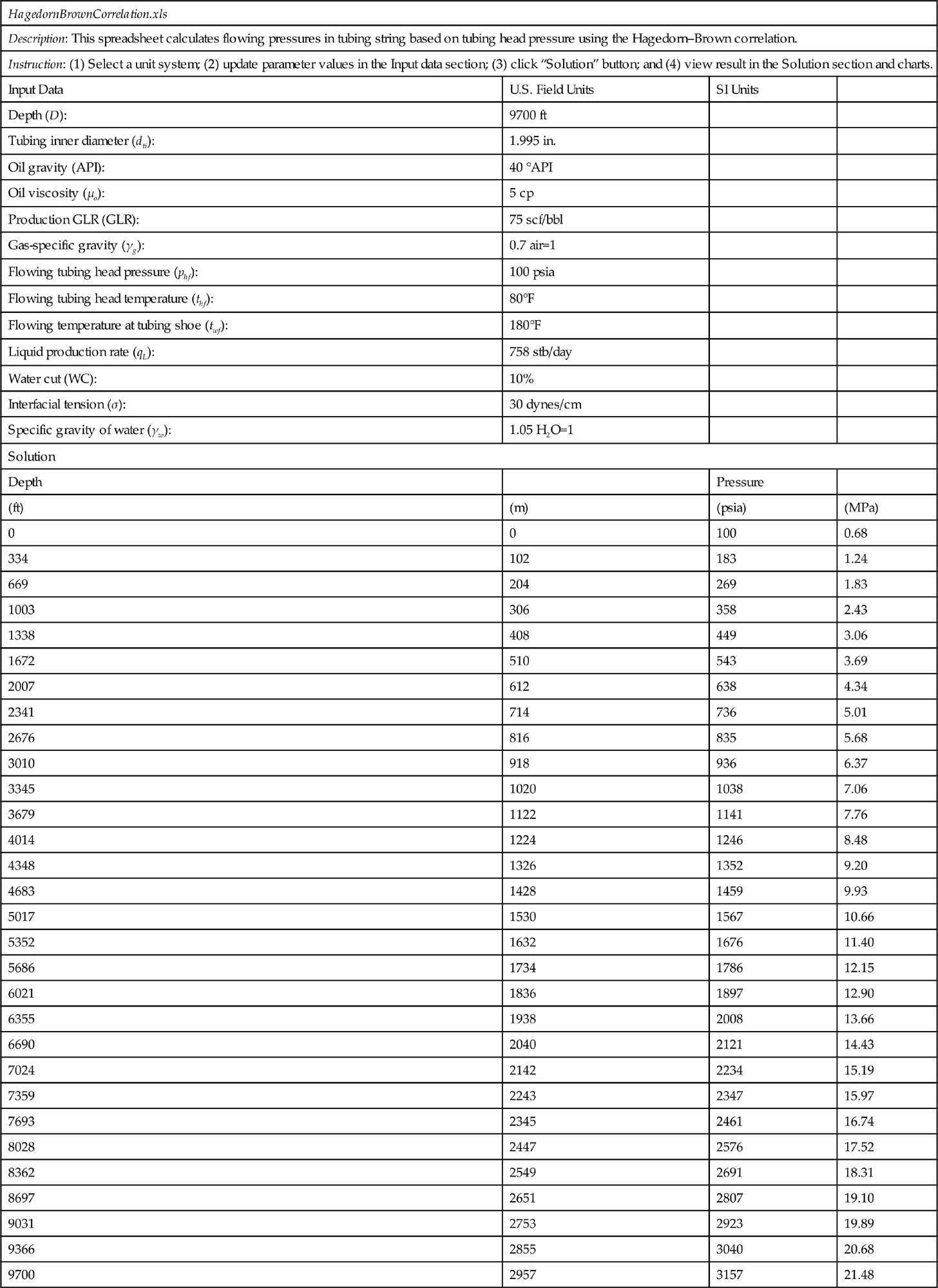
To speed up calculations, the Hagedorn–Brown correlation has been coded in the spreadsheet program Hagedorn Brown Correlation.xls.
Example Problem 4.6 For the data given below, calculate and plot pressure traverse in the tubing string:
| Tubing shoe depth: | 9700 ft |
| Tubing inner diameter: | 1.995 in. |
| Oil gravity: | 40 °API |
| Oil viscosity: | 5 cp |
| Production GLR: | 75 scf/bbl |
| Gas-specific gravity: | 0.7 air=1 |
| Flowing tubing head pressure: | 100 psia |
| Flowing tubing head temperature: | 80°F |
| Flowing temperature at tubing shoe: | 180°F |
| Liquid production rate: | 758 stb/day |
| Water cut: | 10% |
| Interfacial tension: | 30 dynes/cm |
| Specific gravity of water: | 1.05 H2O=1 |
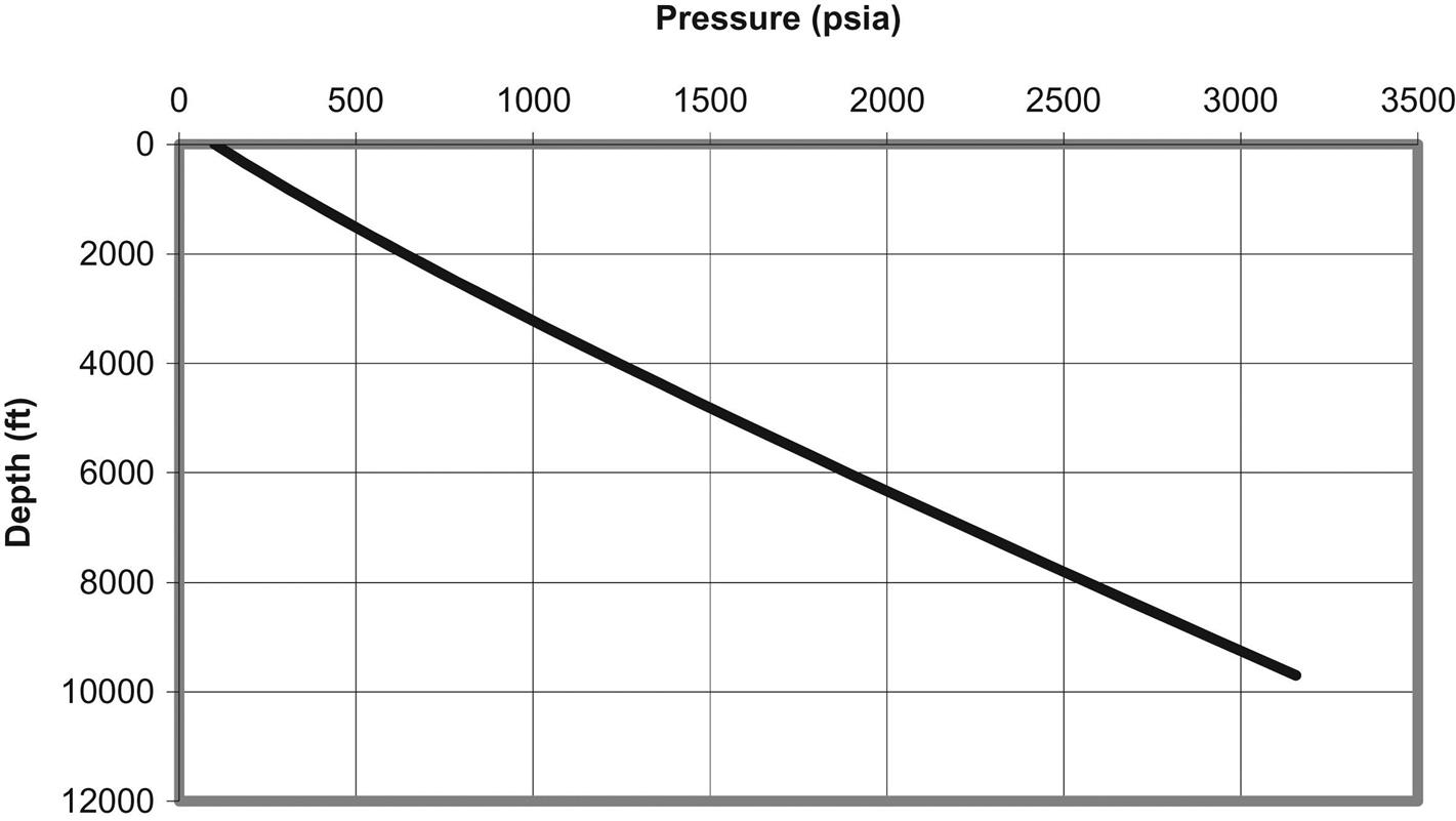
Solution This example problem is solved with the spreadsheet program HagedornBrownCorrelation.xls. The result is shown in Table 4.5 and Fig. 4.5.
Table 4.5
Result Given by HagedornBrownCorrelation.xls for Example Problem 4.6
| HagedornBrownCorrelation.xls | |||
| Description: This spreadsheet calculates flowing pressures in tubing string based on tubing head pressure using the Hagedorn–Brown correlation. | |||
| Instruction: (1) Select a unit system; (2) update parameter values in the Input data section; (3) click “Solution” button; and (4) view result in the Solution section and charts. | |||
| Input Data | U.S. Field Units | SI Units | |
| Depth (D): | 9700 ft | ||
| Tubing inner diameter (dti): | 1.995 in. | ||
| Oil gravity (API): | 40 °API | ||
| Oil viscosity (μo): | 5 cp | ||
| Production GLR (GLR): | 75 scf/bbl | ||
| Gas-specific gravity (γg): | 0.7 air=1 | ||
| Flowing tubing head pressure (phf): | 100 psia | ||
| Flowing tubing head temperature (thf): | 80°F | ||
| Flowing temperature at tubing shoe (twf): | 180°F | ||
| Liquid production rate (qL): | 758 stb/day | ||
| Water cut (WC): | 10% | ||
| Interfacial tension (σ): | 30 dynes/cm | ||
| Specific gravity of water (γw): | 1.05 H2O=1 | ||
| Solution | |||
| Depth | Pressure | ||
| (ft) | (m) | (psia) | (MPa) |
| 0 | 0 | 100 | 0.68 |
| 334 | 102 | 183 | 1.24 |
| 669 | 204 | 269 | 1.83 |
| 1003 | 306 | 358 | 2.43 |
| 1338 | 408 | 449 | 3.06 |
| 1672 | 510 | 543 | 3.69 |
| 2007 | 612 | 638 | 4.34 |
| 2341 | 714 | 736 | 5.01 |
| 2676 | 816 | 835 | 5.68 |
| 3010 | 918 | 936 | 6.37 |
| 3345 | 1020 | 1038 | 7.06 |
| 3679 | 1122 | 1141 | 7.76 |
| 4014 | 1224 | 1246 | 8.48 |
| 4348 | 1326 | 1352 | 9.20 |
| 4683 | 1428 | 1459 | 9.93 |
| 5017 | 1530 | 1567 | 10.66 |
| 5352 | 1632 | 1676 | 11.40 |
| 5686 | 1734 | 1786 | 12.15 |
| 6021 | 1836 | 1897 | 12.90 |
| 6355 | 1938 | 2008 | 13.66 |
| 6690 | 2040 | 2121 | 14.43 |
| 7024 | 2142 | 2234 | 15.19 |
| 7359 | 2243 | 2347 | 15.97 |
| 7693 | 2345 | 2461 | 16.74 |
| 8028 | 2447 | 2576 | 17.52 |
| 8362 | 2549 | 2691 | 18.31 |
| 8697 | 2651 | 2807 | 19.10 |
| 9031 | 2753 | 2923 | 19.89 |
| 9366 | 2855 | 3040 | 20.68 |
| 9700 | 2957 | 3157 | 21.48 |
4.5 Summary
This chapter presented and illustrated different mathematical models for describing wellbore/tubing performance. Among many models, the mH-B model has been found to give results with good accuracy. The industry practice is to conduct a flow gradient (FG) survey to measure the flowing pressures along the tubing string. The FG data are then employed to validate one of the models and tune the model if necessary before the model is used on a large scale.
Problems
4.1. Suppose that 1000 bbl/day of 16 °API, 5-cp oil is being produced through 2⅞-in., 8.6-lbm/ft tubing in a well that is 3° from vertical. If the tubing wall relative roughness is 0.001, assuming no free gas in tubing string, calculate the pressure drop over 1000 ft of tubing.
4.2. For the following given data, calculate bottom-hole pressure using the Poettmann–Carpenter method:
| Tubing head pressure: | 300 psia |
| Tubing head temperature: | 100°F |
| Tubing inner diameter: | 1.66 in. |
| Tubing shoe depth (near bottom hole): | 8000 ft |
| Bottom-hole temperature: | 170°F |
| Liquid production rate: | 2000 stb/day |
| Water cut: | 30% |
| Producing GLR: | 800 scf/stb |
| Oil gravity: | 40 °API |
| Water-specific gravity: | 1.05 1 for freshwater |
| Gas-specific gravity: | 0.70 1 for air |
4.3. For the data given below, estimate bottom-hole pressure with the Guo–Ghalambor method.
| Total measured depth: | 8000 ft |
| The average inclination angle: | 5° |
| Tubing inner diameter: | 1.995 in. |
| Gas production rate: | 0.5 MMscfd |
| Gas-specific gravity: | 0.75 air=1 |
| Oil production rate: | 2000 stb/d |
| Oil-specific gravity: | 0.85 H2O=1 |
| Water production rate: | 500 bbl/d |
| Water-specific gravity: | 1.05 H2O=1 |
| Solid production rate: | 4 ft3/d |
| Solid-specific gravity: | 2.65 H2O=1 |
| Tubing head temperature: | 100°F |
| Bottom-hole temperature: | 170°F |
| Tubing head pressure: | 500 psia |
| Tubing shoe depth: | 6000 ft |
| Tubing inner diameter: | 1.995 in. |
| Oil gravity: | 30 °API |
| Oil viscosity: | 2 cp |
| Production GLR: | 500 scf/bbl |
| Gas-specific gravity: | 0.65 air=1 |
| Flowing tubing head pressure: | 100 psia |
| Flowing tubing head temperature: | 80°F |
| Flowing temperature at tubing shoe: | 140°F |
| Liquid production rate: | 1500 stb/day |
| Water cut: | 20% |
| Interfacial tension: | 30 dynes/cm |
| Specific gravity of water: | 1.05 H2O=1 |
4.4. For the data given below, calculate and plot pressure traverse in the tubing string using the Hagedorn–Brown correlation:
4.5. Suppose 3 MMscf/d of 0.75 specific gravity gas is produced through a 31/2-in. tubing string set to the top of a gas reservoir at a depth of 8000 ft. At the tubing head, the pressure is 1000 psia and the temperature is 120°F; the bottom-hole temperature is 180°F. The relative roughness of tubing is about 0.0006. Calculate the flowing bottom-hole pressure with three methods: (1) the average temperature and compressibility factor method; (2) the Cullender–Smith method; and (3) the four-phase flow method. Make comments on your results.
4.6. Solve Problem 4.5 for gas production through a K-55, 17-lb/ft, 51/2-in casing.
4.7. Suppose 2 MMscf/d of 0.65 specific gravity gas is produced through a 27/8-in. (2.259-in. inside diameter) tubing string set to the top of a gas reservoir at a depth of 5000 ft. Tubing head pressure is 300 psia and the temperature is 100°F; the bottom-hole temperature is 150°F. The relative roughness of tubing is about 0.0006. Calculate the flowing bottom pressure with the average temperature and compressibility factor method.