
Sucker Rod Pumping
Abstract
Sucker rod pumping, also referred to as “beam pumping,” provides mechanical energy to lift oil from bottom-hole to surface. It is efficient, simple, and easy for field people to operate, and can be used to pump a well at very low bottom-hole pressure to maximize oil production rates. It is applicable to slim holes, multiple completions, and high-temperature and viscous oils. The major disadvantages of beam pumping include excessive friction in crooked/deviated holes, solid-sensitive problems, low efficiency in gassy wells, limited depth due to rod capacity, and bulky in offshore operations. Beam pumping trends include improved pump-off controllers, better gas separation, gas handling pumps, and optimization using surface and bottom-hole cards. This chapter presents the principles of sucker rod pumping systems and illustrates a procedure for selecting components of rod pumping systems. Major tasks include calculations of polished rod load, peak torque, stresses in the rod string, pump deliverability, and counterweight placement.
Keywords
Rod; pump; load; torque; efficiency
16.1 Introduction
Sucker rod pumping is also referred to as “beam pumping.” It provides mechanical energy to lift oil from bottom-hole to surface. It is efficient, simple, and easy for field people to operate. It can pump a well down to very low pressure to maximize oil production rate. It is applicable to slim holes, multiple completions, and high-temperature and viscous oils. The system is also easy to change to other wells with minimum cost. The major disadvantages of beam pumping include excessive friction in crooked/deviated holes, solid-sensitive problems, low efficiency in gassy wells, limited depth due to rod capacity, and bulky in offshore operations. Beam pumping trends include improved pump-off controllers, better gas separation, gas handling pumps, and optimization using surface and bottom-hole cards.
16.2 Pumping System
As shown in Fig. 16.1, a sucker rod pumping system consists of a pumping unit at surface and a plunger pump submerged in the production liquid in the well.
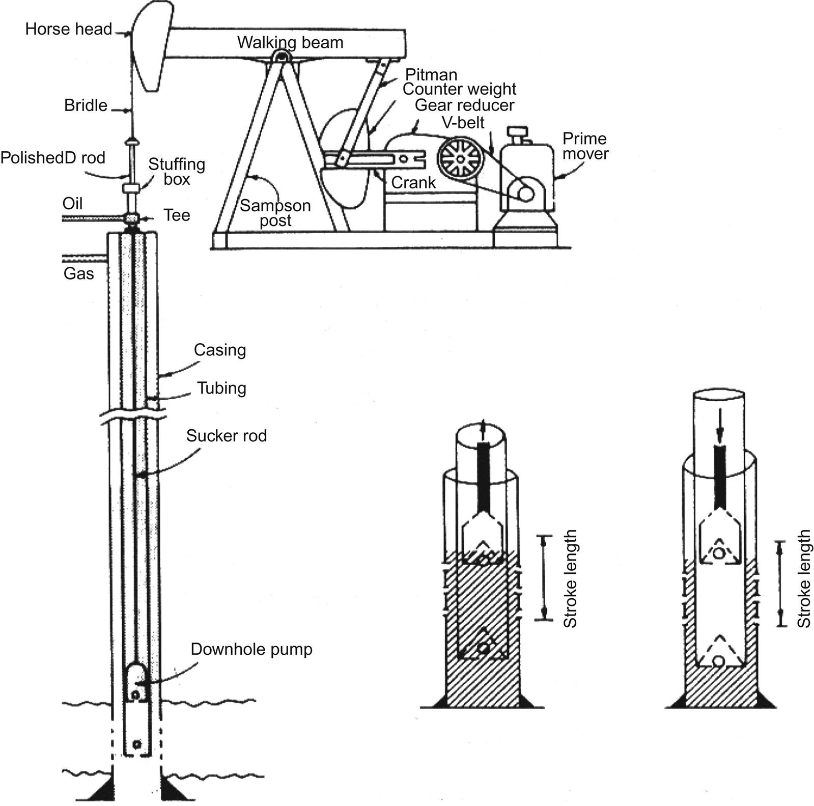
The prime mover is either an electric motor or an internal combustion engine. The modern method is to supply each well with its own motor or engine. Electric motors are most desirable because they can easily be automated. The power from the prime mover is transmitted to the input shaft of a gear reducer by a V-belt drive. The output shaft of the gear reducer drives the crank arm at a lower speed (~4–40 revolutions per minute [rpm] depending on well characteristics and fluid properties). The rotary motion of the crank arm is converted to an oscillatory motion by means of the walking beam through a pitman arm. The horse's head and the hanger cable arrangement is used to ensure that the upward pull on the sucker rod string is vertical at all times (thus, no bending moment is applied to the stuffing box). The polished rod and stuffing box combine to maintain a good liquid seal at the surface and, thus, force fluid to flow into the “T” connection just below the stuffing box.
Conventional pumping units are available in a wide range of sizes, with stroke lengths varying from 12 to almost 200 in. The strokes for any pumping unit type are available in increments (unit size). Within each unit size, the stroke length can be varied within limits (about six different lengths being possible). These different lengths are achieved by varying the position of the pitman arm connection on the crank arm.
Walking beam ratings are expressed in allowable polished rod loads (PRLs) and vary from approximately 3000–35,000 lb. Counterbalance for conventional pumping units is accomplished by placing weights directly on the beam (in smaller units) or by attaching weights to the rotating crank arm (or a combination of the two methods for larger units). In more recent designs, the rotary counterbalance can be adjusted by shifting the position of the weight on the crank by a jackscrew or rack and pinion mechanism.
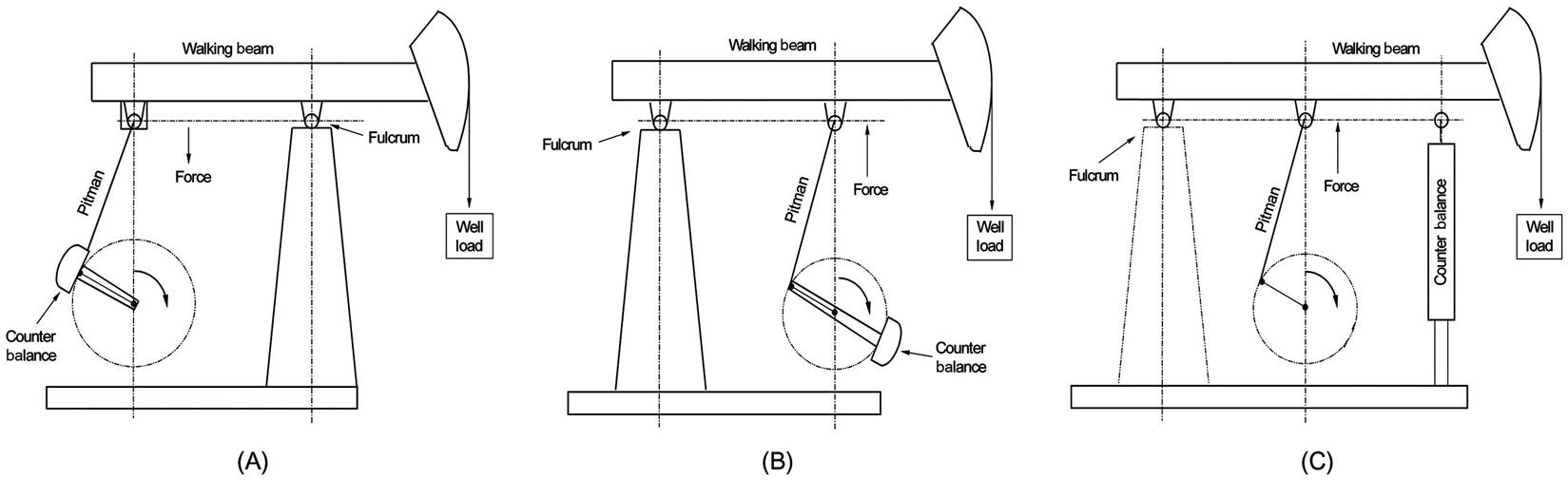
There are two other major types of pumping units. These are the Lufkin Mark II and the Air-Balanced Units (Fig. 16.2). The pitman arm and horse's head are in the same side of the walking beam in these two types of units (Class III lever system). Instead of using counterweights in Lufkin Mark II type units, air cylinders are used in the air-balanced units to balance the torque on the crankshaft.
The American Petroleum Institute (API) has established designations for sucker rod pumping units using a string of characters containing four fields. For example,
The first field is the code for type of pumping unit. C is for conventional units, A is for air-balanced units, B is for beam counterbalance units, and M is for Mark II units. The second field is the code for peak torque rating in thousands of inch-pounds and gear reducer. D stands for double-reduction gear reducer. The third field is the code for PRL rating in hundreds of pounds. The last field is the code for stroke length in inches.
Fig. 16.3 illustrates the working principle of a plunger pump. The pump is installed in the tubing string below the dynamic liquid level. It consists of a working barrel and liner, standing valve (SV), and traveling valve (TV) at the bottom of the plunger, which is connected to sucker rods.
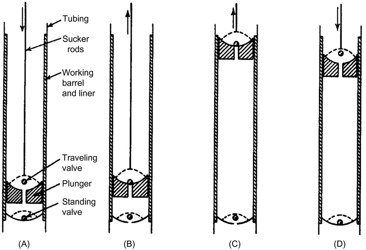
As the plunger is moved downward by the sucker rod string, the TV is open, which allows the fluid to pass through the valve, which lets the plunger move to a position just above the SV. During this downward motion of the plunger, the SV is closed; thus, the fluid is forced to pass through the TV.
When the plunger is at the bottom of the stroke and starts an upward stroke, the TV closes and the SV opens. As upward motion continues, the fluid in the well below the SV is drawn into the volume above the SV (fluid passing through the open SV). The fluid continues to fill the volume above the SV until the plunger reaches the top of its stroke.
There are two basic types of plunger pumps: tubing pump and rod pump (Fig. 16.4). For the tubing pump, the working barrel or liner (with the SV) is made up (i.e., attached) to the bottom of the production tubing string and must be run into the well with the tubing. The plunger (with the TV) is run into the well (inside the tubing) on the sucker rod string. Once the plunger is seated in the working barrel, pumping can be initiated. A rod pump (both working barrel and plunger) is run into the well on the sucker rod string and is seated on a wedged type seat that is fixed to the bottom joint of the production tubing. Plunger diameters vary from ⅝ to 4⅝ in. Plunger area varies from 0.307 in.2 to 17.721 in.2.

16.3 Polished Rod Motion
The theory of polished rod motion has been established since the 1950s (Nind, 1964). Fig. 16.5 shows the cyclic motion of a polished rod in its movements through the stuffing box of the conventional pumping unit and the air-balanced pumping unit.

16.3.1 Conventional Pumping Unit
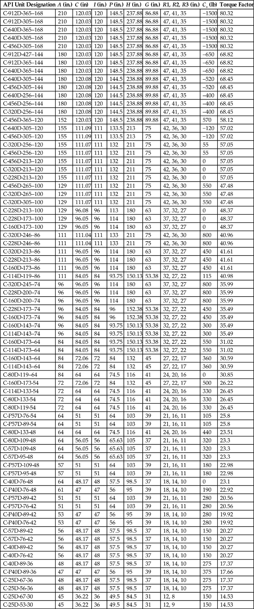
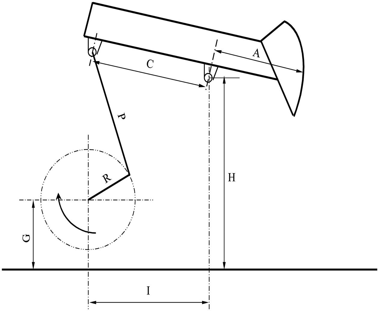
For this type of unit, the acceleration at the bottom of the stroke is somewhat greater than true simple harmonic acceleration. At the top of the stroke, it is less. This is a major drawback for the conventional unit. Just at the time the TV is closing and the fluid load is being transferred to the rods, the acceleration for the rods is at its maximum. These two factors combine to create a maximum stress on the rods that becomes one of the limiting factors in designing an installation. Table 16.1 shows dimensions of some API conventional pumping units. Parameters are defined in Fig. 16.6.
Table 16.1
Conventional Pumping Unit API Geometry Dimensions
| API Unit Designation | A (in.) | C (in) | I (in.) | P (in.) | H (in.) | G (in.) | R1, R2, R3 (in.) | Cs (lb) | Torque Factor |
| C-912D-365–168 | 210 | 120.03 | 120 | 148.5 | 237.88 | 86.88 | 47, 41, 35 | −1500 | 80.32 |
| C-912D-305–168 | 210 | 120.03 | 120 | 148.5 | 237.88 | 86.88 | 47, 41, 35 | −1500 | 80.32 |
| C-640D-365–168 | 210 | 120.03 | 120 | 148.5 | 237.88 | 86.88 | 47, 41, 35 | −1500 | 80.32 |
| C-640D-305–168 | 210 | 120.03 | 120 | 148.5 | 237.88 | 86.88 | 47, 41, 35 | −1500 | 80.32 |
| C-456D-305–168 | 210 | 120.03 | 120 | 148.5 | 237.88 | 86.88 | 47, 41, 35 | −1500 | 80.32 |
| C-912D-427–144 | 180 | 120.03 | 120 | 148.5 | 237.88 | 86.88 | 47, 41, 35 | –650 | 68.82 |
| C-912D-365–144 | 180 | 120.03 | 120 | 148.5 | 237.88 | 86.88 | 47, 41, 35 | –650 | 68.82 |
| C-640D-365–144 | 180 | 120.03 | 120 | 148.5 | 238.88 | 89.88 | 47, 41, 35 | –650 | 68.82 |
| C-640D-305–144 | 180 | 120.08 | 120 | 144.5 | 238.88 | 89.88 | 47, 41, 35 | –520 | 68.45 |
| C-456D-305–144 | 180 | 120.08 | 120 | 144.5 | 238.88 | 89.88 | 47, 41, 35 | –520 | 68.45 |
| C-640D-256–144 | 180 | 120.08 | 120 | 144.5 | 238.88 | 89.88 | 47, 41, 35 | –400 | 68.45 |
| C-456D-256–144 | 180 | 120.08 | 120 | 144.5 | 238.88 | 89.88 | 47, 41, 35 | –400 | 68.45 |
| C-320D-256–144 | 180 | 120.08 | 120 | 144.5 | 238.88 | 89.88 | 47, 41, 35 | –400 | 68.45 |
| C-456D-365–120 | 152 | 120.03 | 120 | 148.5 | 238.88 | 89.88 | 47, 41, 35 | 570 | 58.12 |
| C-640D-305–120 | 155 | 111.09 | 111 | 133.5 | 213 | 75 | 42, 36, 30 | −120 | 57.02 |
| C-456D-305–120 | 155 | 111.09 | 111 | 133.5 | 213 | 75 | 42, 36, 30 | −120 | 57.02 |
| C-320D-256–120 | 155 | 111.07 | 111 | 132 | 211 | 75 | 42, 36, 30 | 55 | 57.05 |
| C-456D-256–120 | 155 | 111.07 | 111 | 132 | 211 | 75 | 42, 36, 30 | 55 | 57.05 |
| C-456D-213–120 | 155 | 111.07 | 111 | 132 | 211 | 75 | 42, 36, 30 | 0 | 57.05 |
| C-320D-213–120 | 155 | 111.07 | 111 | 132 | 211 | 75 | 42, 36, 30 | 0 | 57.05 |
| C-228D-213–120 | 155 | 111.07 | 111 | 132 | 211 | 75 | 42, 36, 30 | 0 | 57.05 |
| C-456D-265–100 | 129 | 111.07 | 111 | 132 | 211 | 75 | 42, 36, 30 | 550 | 47.48 |
| C-320D-265–100 | 129 | 111.07 | 111 | 132 | 211 | 75 | 42, 36, 30 | 550 | 47.48 |
| C-320D-305–100 | 129 | 111.07 | 111 | 132 | 211 | 75 | 42, 36, 30 | 550 | 47.48 |
| C-228D-213–100 | 129 | 96.08 | 96 | 113 | 180 | 63 | 37, 32, 27 | 0 | 48.37 |
| C-228D-173–100 | 129 | 96.05 | 96 | 114 | 180 | 63 | 37, 32, 27 | 0 | 48.37 |
| C-160D-173–100 | 129 | 96.05 | 96 | 114 | 180 | 63 | 37, 32, 27 | 0 | 48.37 |
| C-320D-246–86 | 111 | 111.04 | 111 | 133 | 211 | 75 | 42, 36, 30 | 800 | 40.96 |
| C-228D-246–86 | 111 | 111.04 | 111 | 133 | 211 | 75 | 42, 36, 30 | 800 | 40.96 |
| C-320D-213–86 | 111 | 96.05 | 96 | 114 | 180 | 63 | 37, 32, 27 | 450 | 41.61 |
| C-228D-213–86 | 111 | 96.05 | 96 | 114 | 180 | 63 | 37, 32, 27 | 450 | 41.61 |
| C-160D-173–86 | 111 | 96.05 | 96 | 114 | 180 | 63 | 37, 32, 27 | 450 | 41.61 |
| C-114D-119–86 | 111 | 84.05 | 84 | 93.75 | 150.13 | 53.38 | 32, 27, 22 | 115 | 40.98 |
| C-320D-245–74 | 96 | 96.05 | 96 | 114 | 180 | 63 | 37, 32, 27 | 800 | 35.99 |
| C-228D-200–74 | 96 | 96.05 | 96 | 114 | 180 | 63 | 37, 32, 27 | 800 | 35.99 |
| C-160D-200–74 | 96 | 96.05 | 96 | 114 | 180 | 63 | 37, 32, 27 | 800 | 35.99 |
| C-228D-173–74 | 96 | 84.05 | 84 | 96 | 152.38 | 53.38 | 32, 27, 22 | 450 | 35.49 |
| C-160D-173–74 | 96 | 84.05 | 84 | 96 | 152.38 | 53.38 | 32, 27, 22 | 450 | 35.49 |
| C-160D-143–74 | 96 | 84.05 | 84 | 93.75 | 150.13 | 53.38 | 32, 27, 22 | 300 | 35.49 |
| C-114D-143–74 | 96 | 84.05 | 84 | 93.75 | 150.13 | 53.38 | 32, 27, 22 | 300 | 35.49 |
| C-160D-173–64 | 84 | 84.05 | 84 | 93.75 | 150.13 | 53.38 | 32, 27, 22 | 550 | 31.02 |
| C-114D-173–64 | 84 | 84.05 | 84 | 93.75 | 150.13 | 53.38 | 32, 27, 22 | 550 | 31.02 |
| C-160D-143–64 | 84 | 72.06 | 72 | 84 | 132 | 45 | 27, 22, 17 | 360 | 30.59 |
| C-114D-143–64 | 84 | 72.06 | 72 | 84 | 132 | 45 | 27, 22, 17 | 360 | 30.59 |
| C-80D-119–64 | 84 | 64 | 64 | 74.5 | 116 | 41 | 24, 20, 16 | 0 | 30.85 |
| C-160D-173-54 | 72 | 72.06 | 72 | 84 | 132 | 45 | 27, 22, 17 | 500 | 26.22 |
| C-114D-133-54 | 72 | 64 | 64 | 74.5 | 116 | 41 | 24, 20, 16 | 330 | 26.45 |
| C-80D-133-54 | 72 | 64 | 64 | 74.5 | 116 | 41 | 24, 20, 16 | 330 | 26.45 |
| C-80D-119-54 | 72 | 64 | 64 | 74.5 | 116 | 41 | 24, 20, 16 | 330 | 26.45 |
| C-P57D-76-54 | 64 | 51 | 51 | 64 | 103 | 39 | 21, 16, 11 | 105 | 25.8 |
| C-P57D-89-54 | 64 | 51 | 51 | 64 | 103 | 39 | 21, 16, 11 | 105 | 25.8 |
| C-80D-133-48 | 64 | 64 | 64 | 74.5 | 116 | 41 | 24, 20, 16 | 440 | 23.51 |
| C-80D-109-48 | 64 | 56.05 | 56 | 65.63 | 105 | 37 | 21, 16, 11 | 320 | 23.3 |
| C-57D-109-48 | 64 | 56.05 | 56 | 65.63 | 105 | 37 | 21, 16, 11 | 320 | 23.3 |
| C-57D-95-48 | 64 | 56.05 | 56 | 65.63 | 105 | 37 | 21, 16, 11 | 320 | 23.3 |
| C-P57D-109-48 | 57 | 51 | 51 | 64 | 103 | 39 | 21, 16, 11 | 180 | 22.98 |
| C-P57D-95-48 | 57 | 51 | 51 | 64 | 103 | 39 | 21, 16, 11 | 180 | 22.98 |
| C-40D-76-48 | 64 | 48.17 | 48 | 57.5 | 98.5 | 37 | 18, 14, 10 | 0 | 23.1 |
| C-P40D-76-48 | 61 | 47 | 47 | 56 | 95 | 39 | 18, 14, 10 | 190 | 22.92 |
| C-P57D-89-42 | 51 | 51 | 51 | 64 | 103 | 39 | 21, 16, 11 | 280 | 20.56 |
| C-P57D-76-42 | 51 | 51 | 51 | 64 | 103 | 39 | 21, 16, 11 | 280 | 20.56 |
| C-P40D-89-42 | 53 | 47 | 47 | 56 | 95 | 39 | 18, 14, 10 | 280 | 19.92 |
| C-P40D-76-42 | 53 | 47 | 47 | 56 | 95 | 39 | 18, 14, 10 | 280 | 19.92 |
| C-57D-89-42 | 56 | 48.17 | 48 | 57.5 | 98.5 | 37 | 18, 14, 10 | 150 | 20.27 |
| C-57D-76-42 | 56 | 48.17 | 48 | 57.5 | 98.5 | 37 | 18, 14, 10 | 150 | 20.27 |
| C-40D-89-42 | 56 | 48.17 | 48 | 57.5 | 98.5 | 37 | 18, 14, 10 | 150 | 20.27 |
| C-40D-76-42 | 56 | 48.17 | 48 | 57.5 | 98.5 | 37 | 18, 14, 10 | 150 | 20.27 |
| C-40D-89-36 | 48 | 48.17 | 48 | 57.5 | 98.5 | 37 | 18, 14, 10 | 275 | 17.37 |
| C-P40D-89-36 | 47 | 47 | 47 | 56 | 95 | 39 | 18, 14, 10 | 375 | 17.66 |
| C-25D-67-36 | 48 | 48.17 | 48 | 57.5 | 98.5 | 37 | 18, 14, 10 | 275 | 17.37 |
| C-25D-56-36 | 48 | 48.17 | 48 | 57.5 | 98.5 | 37 | 18, 14, 10 | 275 | 17.37 |
| C-25D-67-30 | 45 | 36.22 | 36 | 49.5 | 84.5 | 31 | 12, 8 | 150 | 14.53 |
| C-25D-53-30 | 45 | 36.22 | 36 | 49.5 | 84.5 | 31 | 12, 9 | 150 | 14.53 |
16.3.2 Air-Balanced Pumping Unit
For this type of unit, the maximum acceleration occurs at the top of the stroke (the acceleration at the bottom of the stroke is less than simple harmonic motion). Thus, a lower maximum stress is set up in the rod system during transfer of the fluid load to the rods.
The following analyses of polished rod motion apply to conventional units. Fig. 16.7 illustrates an approximate motion of the connection point between pitman arm and walking beam.

If x denotes the distance of B below its top position C and is measured from the instant at which the crank arm and pitman arm are in the vertical position with the crank arm vertically upward, the law of cosine gives
that is,
where ω is the angular velocity of the crank. The equation reduces to
so that
When ωt is zero, x is also zero, which means that the negative root sign must be taken. Therefore,
Acceleration is
Carrying out the differentiation for acceleration, it is found that the maximum acceleration occurs when ωt is equal to zero (or an even multiple of p radians) and that this maximum value is
(16.1)
It also appears that the minimum value of acceleration is
(16.2)
If N is the number of pumping strokes per minute, then
(16.3)
The maximum downward acceleration of point B (which occurs when the crank arm is vertically upward) is
(16.4)
or
(16.5)
Likewise the minimum upward (amin) acceleration of point B (which occurs when the crank arm is vertically downward) is
(16.6)
It follows that in a conventional pumping unit, the maximum upward acceleration of the horse's head occurs at the bottom of the stroke (polished rod) and is equal to
(16.7)
where d1 and d2 are shown in Fig. 16.5. However,
where S is the polished rod stroke length. So if S is measured in inches, then
or
(16.8)
So substituting Eq. (16.8) into Eq. (16.7) yields
(16.9)
or we can write Eq. (16.9) as
(16.10)
where M is the machinery factor and is defined as
(16.11)
Similarly,
(16.12)
For air-balanced units, because of the arrangements of the levers, the acceleration defined in Eq. (16.12) occurs at the bottom of the stroke, and the acceleration defined in Eq. (16.9) occurs at the top. With the lever system of an air-balanced unit, the polished rod is at the top of its stroke when the crank arm is vertically upward (Fig. 16.5B).
16.4 Load to the Pumping Unit
The load exerted to the pumping unit depends on well depth, rod size, fluid properties, and system dynamics. The maximum PRL and peak torque are major concerns for pumping unit.
16.4.1 Maximum PRL
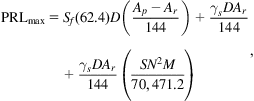
The PRL is the sum of weight of fluid being lifted, weight of plunger, weight of sucker rods string, dynamic load due to acceleration, friction force, and the up-thrust from below on plunger. In practice, no force attributable to fluid acceleration is required, so the acceleration term involves only acceleration of the rods. Also, the friction term and the weight of the plunger are neglected. We ignore the reflective forces, which will tend to underestimate the maximum PRL. To compensate for this, we set the up-thrust force to zero. Also, we assume the TV is closed at the instant at which the acceleration term reaches its maximum. With these assumptions, the PRLmax becomes
(16.13)
 (16.13)
Sf=specific gravity of fluid in tubing
D=length of sucker rod string, ft
Ap=gross plunger cross-sectional area, in.2
Ar=sucker rod cross-sectional area, in.2
γs=specific weight of steel, 490 lb/ft3
M=Eq. (16.11).
Note that for the air-balanced unit, M in Eq. (16.13) is replaced by 1-c/h.
Eq. (16.13) can be rewritten as
(16.14)
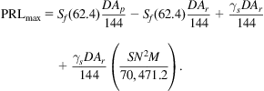 (16.14)
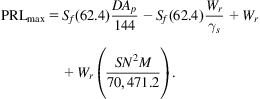
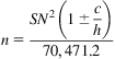
If the weight of the rod string in air is
(16.15)
which can be solved for Ar, which is
(16.16)
Substituting Eq. (16.16) into Eq. (16.14) yields
(16.17)
 (16.17)
The above equation is often further reduced by taking the fluid in the second term (the subtractive term) as a 50 °API with Sf=0.78. Thus, Eq. (16.17) becomes (where γs=490)
or
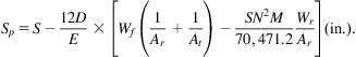
(16.18)
where ![]() and is called the fluid load (not to be confused with the actual fluid weight on the rod string). Thus, Eq. (16.18) can be rewritten as
and is called the fluid load (not to be confused with the actual fluid weight on the rod string). Thus, Eq. (16.18) can be rewritten as
(16.19)
where for conventional units
(16.20)
and for air-balanced units
(16.21)
16.4.2 Minimum PRL
The minimum PRL occurs while the TV is open so that the fluid column weight is carried by the tubing and not the rods. The minimum load is at or near the top of the stroke. Neglecting the weight of the plunger and friction term, the minimum PRL is
which, for 50 °API oil, reduces to
(16.22)
where for the conventional units
(16.23)
and for air-balanced units
(16.24)
16.4.3 Counterweights
To reduce the power requirements for the prime mover, a counterbalance load is used on the walking beam (small units) or the rotary crank. The ideal counterbalance load C is the average PRL. Therefore,
Using Eqs. (16.19) and (16.22) in the above, we get
(16.25)
or for conventional units
(16.26)
and for air-balanced units
(16.27)
The counterbalance load should be provided by structure unbalance and counterweights placed at walking beam (small units) or the rotary crank. The counterweights can be selected from manufacturer's catalog based on the calculated C value. The relationship between the counterbalance load C and the total weight of the counterweights is
16.4.4 Peak Torque and Speed Limit
The peak torque exerted is usually calculated on the most severe possible assumption, which is that the peak load (polished rod less counterbalance) occurs when the effective crank length is also a maximum (when the crank arm is horizontal). Thus, peak torque T is (Fig. 16.5)
(16.28)
Substituting Eq. (16.8) into Eq. (16.28) gives
(16.29)
or
or
(16.30)
Because the pumping unit itself is usually not perfectly balanced (Cs ≠ 0), the peak torque is also affected by structure unbalance. Torque factors are used for correction:
(16.31)
For symmetrical conventional and air-balanced units, TF=TF1=TF2.
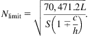
There is a limiting relationship between stroke length and cycles per minute. As given earlier, the maximum value of the downward acceleration (which occurs at the top of the stroke) is equal to
(16.32)
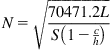
(the ± refers to conventional units or air-balanced units, see Eqs. (16.9) and (16.12)). If this maximum acceleration divided by g exceeds unity, the downward acceleration of the hanger is greater than the free-fall acceleration of the rods at the top of the stroke. This leads to severe pounding when the polished rod shoulder falls onto the hanger (leading to failure of the rod at the shoulder). Thus, a limit of the above downward acceleration term divided by g is limited to approximately 0.5 (or where L is determined by experience in a particular field). Thus,
(16.33)
or
(16.34)
 (16.34)
For L=0.5,
(16.35)
 (16.35)
The minus sign is for conventional units and the plus sign for air-balanced units.
16.4.5 Tapered Rod Strings
For deep well applications, it is necessary to use tapered sucker rod strings to reduce the PRL at the surface. The larger diameter rod is placed at the top of the rod string, then the next largest, and then the least largest. Usually these are in sequences up to four different rod sizes. The tapered rod strings are designated by 1/8-in. (in diameter) increments. Tapered rod strings can be identified by their numbers, such as:
1. No. 88 is a non-tapered ![]() - or 1-in. diameter rod string
- or 1-in. diameter rod string
2. No. 76 is a tapered string with ⅞-in. diameter rod at the top, then a ![]() -in. diameter rod at the bottom.
-in. diameter rod at the bottom.
3. No. 75 is a three-way tapered string consisting of
b. ![]() -in. diameter rod at middle
-in. diameter rod at middle
c. ![]() -in. diameter rod at bottom
-in. diameter rod at bottom
4. No. 107 is a four-way tapered string consisting of
a. ![]() -in. (or 1¼-in.) diameter rod at top
-in. (or 1¼-in.) diameter rod at top
b. ![]() -in. (or 1⅛-in.) diameter rod below
-in. (or 1⅛-in.) diameter rod below ![]() -in. diameter rod
-in. diameter rod
Tapered rod strings are designed for static (quasi-static) lads with a sufficient factor of safety to allow for random low-level dynamic loads. Two criteria are used in the design of tapered rod strings:
1. Stress at the top rod of each rod size is the same throughout the string.
2. Stress in the top rod of the smallest (deepest) set of rods should be the highest (~30,000 psi) and the stress progressively decreases in the top rods of the higher sets of rods.
The reason for the second criterion is that it is preferable that any rod breaks occur near the bottom of the string (otherwise macaroni).
ExampleProblem 16.1 The following geometric dimensions are for the pumping unit C–320D–213–86:
If this unit is used with a 2½-in. plunger and ⅞-in. rods to lift 25 °API gravity crude (formation volume factor 1.2 rb/stb) at depth of 3000 ft, answer the following questions:
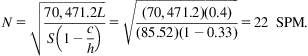
1. What is the maximum allowable pumping speed if L=0.4 is used?
2. What is the expected maximum PRL?
3. What is the expected peak torque?
4. What is the desired counterbalance weight to be placed at the maximum position on the crank?
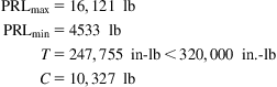
Solution The pumping unit C–320D–213–86 has a peak torque of gearbox rating of 320,000 in.-lb, a polished rod rating of 21,300 lb, and a maximum polished rod stroke of 86 in.
1. Based on the configuration for conventional unit shown in Fig. 16.5A and Table 16.1, the polished rod stroke length can be estimated as
The maximum allowable pumping speed is
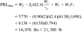
2. The maximum PRL can be calculated with Eq. (16.17). The 25 °API gravity has an Sf=0.9042. The area of the 2½-in. plunger is Ap=4.91 in.2. The area of the ⅞-in. rod is Ar=0.60 in.2. Then
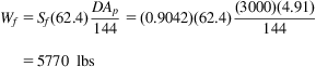
Then the expected maximum PRL is
3. The peak torque is calculated by Eq. (16.30):

4. Accurate calculation of counterbalance load requires the minimum PRL:
A product catalog of LUFKIN Industries indicates that the structure unbalance is 450 lb and 4 No. 5ARO counterweights placed at the maximum position (c in this case) on the crank will produce an effective counterbalance load of 10,160 lb, that is,
which gives Wc=11,221 lb. To generate the ideal counterbalance load of C=9526 lb, the counterweights should be placed on the crank at
The computer program SuckerRodPumpingLoad.xls can be used for quickly seeking solutions to similar problems. It is available from the publisher with this book. The solution is shown in Table 16.2.
Table 16.2
Solution Given by Computer Program SuckerRodPumpingLoad.xls
| SuckerRodPumpingLoad.xls | |
| Description: This spreadsheet calculates the maximum allowable pumping speed, the maximum PRL, the minimum PRL, peak torque, and counterbalance load. | |
| Instruction: (1) Update parameter values in the Input section; and (2) view result in the Solution section. | |
| Input Data | |
| Pump setting depth (D): | 3000 ft |
| Plunger diameter (dp): | 2.5 in. |
| Rod section 1, diameter (dr1): | 1 in. |
| Length (L1): | 0 ft |
| Rod section 2, diameter (dr2): | 0.875 in. |
| Length (L2): | 3000 ft |
| Rod section 3, diameter (dr3): | 0.75 in. |
| Length (L3): | 0 ft |
| Rod section 4, diameter (dr4): | 0.5 in. |
| Length (L4): | 0 ft |
| Type of pumping unit (1=conventional; −1=Mark II or Air-balanced): | 1 |
| Beam dimension 1 (d1) | 96.05 in. |
| Beam dimension 2 (d2) | 111 in. |
| Crank length (c): | 37 in. |
| Crank to pitman ratio (c/h): | 0.33 |
| Oil gravity (API): | 25 °API |
| Maximum allowable acceleration factor (L): | 0.4 |
| Solution | |
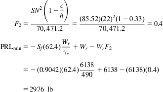
| =85.52 in. | |
 |
=22 spm |
| =4.91 in.2 | |
| =0.60 in. | |
| =5770 lb | |
| =6138 lb | |
| =0.7940° | |
| =16,076 lb | |
| =280,056 lb | |
| =0.40 | |
| =2976 lb | |
| =9526 lb | |

16.5 Pump Deliverability and Power Requirements
Liquid flow rate delivered by the plunger pump can be expressed as
or
where Sp is the effective plunger stroke length (in.), Ev is the volumetric efficiency of the plunger, and Bo formation volume factor of the fluid.
16.5.1 Effective Plunger Stroke Length
The motion of the plunger at the pump setting depth and the motion of the polished rod do not coincide in time and in magnitude because sucker rods and tubing strings are elastic. Plunger motion depends on a number of factors including polished rod motion, sucker rod stretch, and tubing stretch. The theory in this subject has been well established (Nind, 1964).
Two major sources of difference in the motion of the polished rod and the plunger are elastic stretch (elongation) of the rod string and overtravel. Stretch is caused by the periodic transfer of the fluid load from the SV to the TV and back again. The result is a function of the stretch of the rod string and the tubing string. Rod string stretch is caused by the weight of the fluid column in the tubing coming on to the rod string at the bottom of the stroke when the TV closes (this load is removed from the rod string at the top of the stroke when the TV opens). It is apparent that the plunger stroke will be less than the polished rod stroke length S by an amount equal to the rod stretch. The magnitude of the rod stretch is
(16.36)
Tubing stretch can be expressed by a similar equation:
(16.37)
But because the tubing cross-sectional area At is greater than the rod cross-sectional area Ar, the stretch of the tubing is small and is usually neglected. However, the tubing stretch can cause problems with wear on the casing. Thus, for this reason a tubing anchor is almost always used.
Plunger overtravel at the bottom of the stroke is a result of the upward acceleration imposed on the downward-moving sucker rod elastic system. An approximation to the extent of the overtravel may be obtained by considering a sucker rod string being accelerated vertically upward at a rate n times the acceleration of gravity. The vertical force required to supply this acceleration is nWr. The magnitude of the rod stretch due to this force is
(16.38)
But the maximum acceleration term n can be written as
so that Eq. (16.38) becomes
(16.39)
 (16.39)
where again the plus sign applies to conventional units and the minus sign to air-balanced units.
Let us restrict our discussion to conventional units. Then Eq. (16.39) becomes
(16.40)
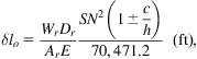
Eq. (16.40) can be rewritten to yield δlo in inches. Wr is
and γS=490 lb/ft3 with E=30×106 lb/m2. Eq. (16.40) becomes
(16.41)
which is the familiar Coberly expression for overtravel (Coberly, 1938).
Plunger stroke is approximated using the above expressions as
or
(16.42)
 (16.42)
If pumping is carried out at the maximum permissible speed limited by Eq. (16.34), the plunger stroke becomes
(16.43)
 (16.43)
For the air-balanced unit, the term is replaced by its reciprocal.
16.5.2 Volumetric Efficiency
Volumetric efficiency of the plunger mainly depends on the rate of slippage of oil past the pump plunger and the solution–gas ratio under pump condition.
Metal-to-metal plungers are commonly available with plunger-to-barrel clearance on the diameter of −0.001, −0.002, −0.003, −0.004, and −0.005 in. Such fits are referred to as −1, −2, −3, −4, and −5, meaning the plunger outside diameter is 0.001 in. smaller than the barrel inside diameter. In selecting a plunger, one must consider the viscosity of the oil to be pumped. A loose fit may be acceptable for a well with high-viscosity oil (low °API gravity). But such a loose fit in a well with low-viscosity oil may be very inefficient. Guidelines are as follows:
1. Low-viscosity oils (1–20 cps) can be pumped with a plunger to barrel fit of −0.001 in.
2. High-viscosity oils (7400 cps) will probably carry sand in suspension so a plunger-to-barrel fit of approximately 0.005 in. can be used.
An empirical formula has been developed that can be used to calculate the slippage rate, qs (bbl/day), through the annulus between the plunger and the barrel:
(16.44)
dp=plunger outside diameter, in.
db=barrel inside diameter, in.
The value of kp is 2.77×10⁶–6.36×10⁶ depending on field conditions. An average value is 4.17×10⁶. The value of Δp may be estimated on the basis of well productivity index and production rate. A reasonable estimate may be a value that is twice the production drawdown.
Volumetric efficiency can decrease significantly due to the presence of free gas below the plunger. As the fluid is elevated and gas breaks out of solution, there is a significant difference between the volumetric displacement of the bottom-hole pump and the volume of the fluid delivered to the surface. This effect is denoted by the shrinkage factor greater than 1.0, indicating that the bottom-hole pump must displace more fluid by some additional percentage than the volume delivered to the surface (Brown, 1980). The effect of gas on volumetric efficiency depends on solution–gas ratio and bottom-hole pressure. Down-hole devices, called “gas anchors,” are usually installed on pumps to separate the gas from the liquid.
In summary, volumetric efficiency is mainly affected by the slippage of oil and free gas volume below plunger. Both effects are difficult to quantify. Pump efficiency can vary over a wide range but are commonly 70%–80%.
16.5.3 Power Requirements
The prime mover should be properly sized to provide adequate power to lift the production fluid, to overcome friction loss in the pump, in the rod string and polished rod, and in the pumping unit. The power required for lifting fluid is called “hydraulic power.” It is usually expressed in terms of net lift:
(16.45)
and
(16.46)
The power required to overcome friction losses can be empirically estimated as
(16.47)
Thus, the required prime mover power can be expressed as
(16.48)
where Fs is a safety factor of 1.25–1.50.
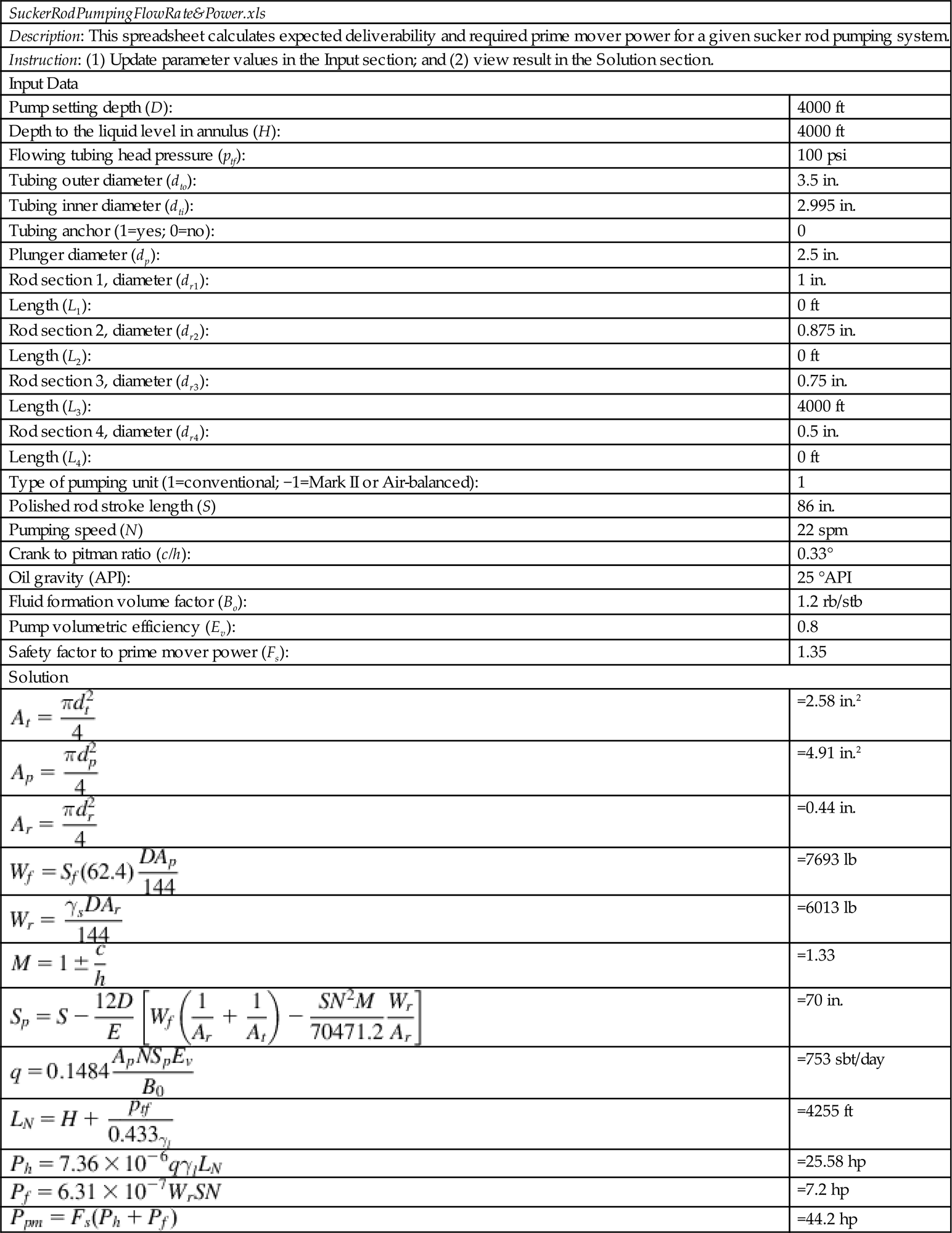
Example Problem 16.2 A well is pumped off (fluid level is the pump depth) with a rod pump described in Example Problem 16.1. A 3-in. tubing string (3.5-in. OD, 2.995 ID) in the well is not anchored. Calculate (1) expected liquid production rate (use pump volumetric efficiency 0.8), and (2) required prime mover power (use safety factor 1.35).
Solution This problem can be quickly solved using the program SuckerRodPumpingFlowrate&Power.xls. The solution is shown in Table 16.3.
Table 16.3
Solution Given by SuckerRodPumpingFlowrate&Power.xls
| SuckerRodPumpingFlowRate&Power.xls | |
| Description: This spreadsheet calculates expected deliverability and required prime mover power for a given sucker rod pumping system. | |
| Instruction: (1) Update parameter values in the Input section; and (2) view result in the Solution section. | |
| Input Data | |
| Pump setting depth (D): | 4000 ft |
| Depth to the liquid level in annulus (H): | 4000 ft |
| Flowing tubing head pressure (ptf): | 100 psi |
| Tubing outer diameter (dto): | 3.5 in. |
| Tubing inner diameter (dti): | 2.995 in. |
| Tubing anchor (1=yes; 0=no): | 0 |
| Plunger diameter (dp): | 2.5 in. |
| Rod section 1, diameter (dr1): | 1 in. |
| Length (L1): | 0 ft |
| Rod section 2, diameter (dr2): | 0.875 in. |
| Length (L2): | 0 ft |
| Rod section 3, diameter (dr3): | 0.75 in. |
| Length (L3): | 4000 ft |
| Rod section 4, diameter (dr4): | 0.5 in. |
| Length (L4): | 0 ft |
| Type of pumping unit (1=conventional; −1=Mark II or Air-balanced): | 1 |
| Polished rod stroke length (S) | 86 in. |
| Pumping speed (N) | 22 spm |
| Crank to pitman ratio (c/h): | 0.33° |
| Oil gravity (API): | 25 °API |
| Fluid formation volume factor (Bo): | 1.2 rb/stb |
| Pump volumetric efficiency (Ev): | 0.8 |
| Safety factor to prime mover power (Fs): | 1.35 |
| Solution | |
| =2.58 in.2 | |
| =4.91 in.2 | |
| =0.44 in. | |
| =7693 lb | |
| =6013 lb | |
| =1.33 | |
| =70 in. | |
| =753 sbt/day | |
| =4255 ft | |
| =25.58 hp | |
| =7.2 hp | |
| =44.2 hp | |
16.6 Procedure for Pumping Unit Selection
The following procedure can be used for selecting a pumping unit:
1. From the maximum anticipated fluid production (based on inflow performance relationship (IPR)) and estimated volumetric efficiency, calculate required pump displacement.
2. Based on well depth and pump displacement, determine API rating and stroke length of the pumping unit to be used. This can be done using either Fig. 16.8 or Table 16.4.
3. Select tubing size, plunger size, rod sizes, and pumping speed from Table 16.4.
4. Calculate the fractional length of each section of the rod string.
5. Calculate the length of each section of the rod string to the nearest 25 ft.
6. Calculate the acceleration factor.
7. Determine the effective plunger stroke length.
8. Using the estimated volumetric efficiency, determine the probable production rate and check it against the desired production rate.
9. Calculate the dead weight of the rod string.
11. Determine peak PRL and check it against the maximum beam load for the unit selected.
12. Calculate the maximum stress at the top of each rod size and check it against the maximum permissible working stress for the rods to be used.
13. Calculate the ideal counterbalance effect and check it against the counterbalance available for the unit selected.
14. From the manufacturer's literature, determine the position of the counterweight to obtain the ideal counterbalance effect.
15. On the assumption that the unit will be no more than 5% out of counterbalance, calculate the peak torque on the gear reducer and check it against the API rating of the unit selected.
16. Calculate hydraulic horsepower, friction horsepower, and brake horsepower of the prime mover. Select the prime mover.
17. From the manufacturer's literature, obtain the gear reduction ratio and unit sheave size for the unit selected, and the speed of the prime mover. From this, determine the engine sheave size to obtain the desired pumping speed.
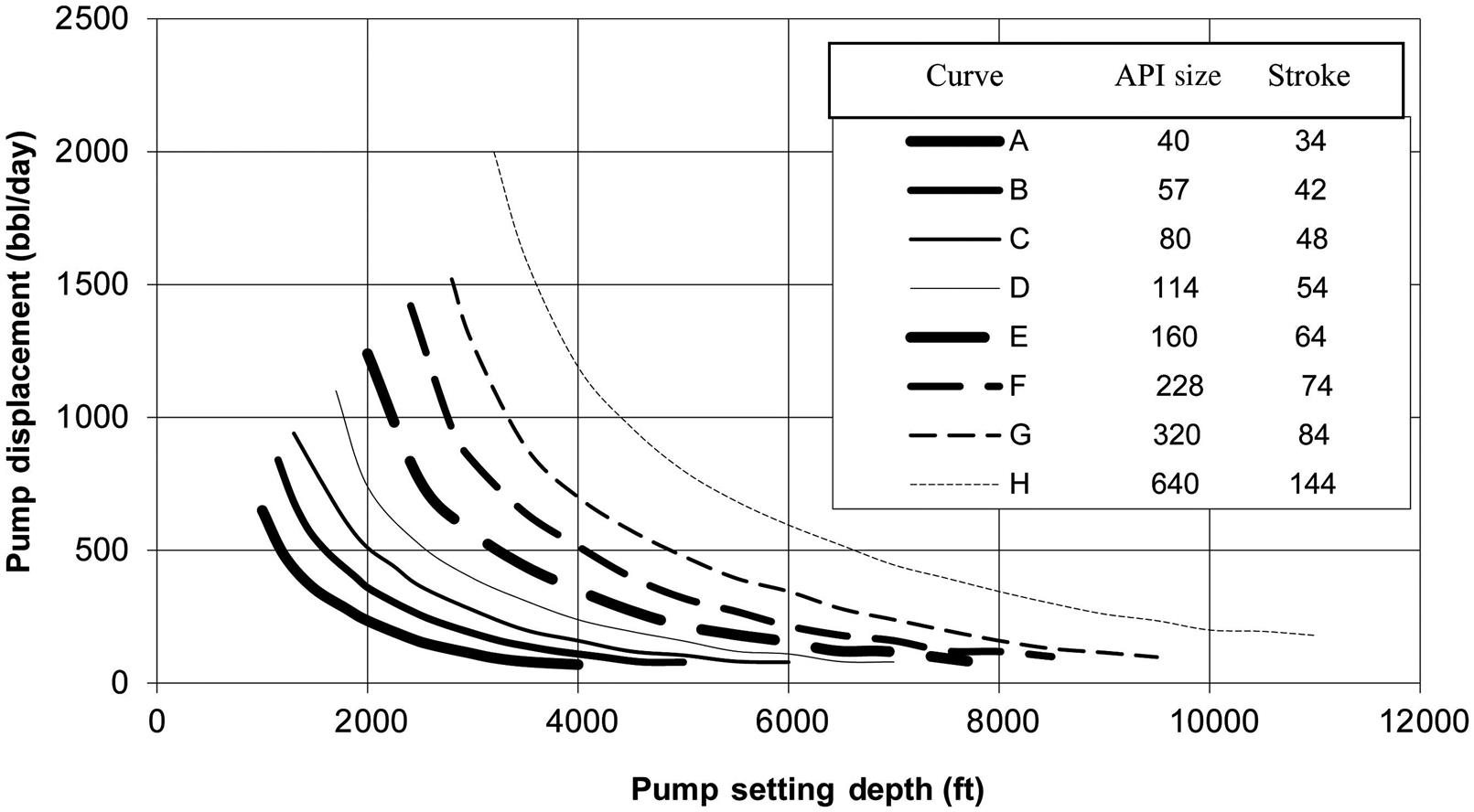
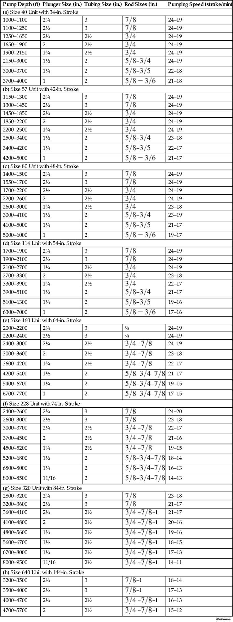
Table 16.4
Design Data for API Sucker Rod Pumping Units
| Pump Depth (ft) | Plunger Size (in.) | Tubing Size (in.) | Rod Sizes (in.) | Pumping Speed (stroke/min) |
| (a) Size 40 Unit with 34-in. Stroke | ||||
| 1000–1100 | 2¾ | 3 | 24–19 | |
| 1100–1250 | 2½ | 3 | 24–19 | |
| 1250–1650 | 2¼ | 2½ | 24–19 | |
| 1650–1900 | 2 | 2½ | 24–19 | |
| 1900–2150 | 1¾ | 2½ | 24–19 | |
| 2150–3000 | 1½ | 2 | 24–19 | |
| 3000–3700 | 1¼ | 2 | 22–18 | |
| 3700–4000 | 1 | 2 | 21–18 | |
| (b) Size 57 Unit with 42-in. Stroke | ||||
| 1150–1300 | 2¾ | 3 | 24–19 | |
| 1300–1450 | 2½ | 3 | 24–19 | |
| 1450–1850 | 2¼ | 2½ | 24–19 | |
| 1850–2200 | 2 | 2½ | 24–19 | |
| 2200–2500 | 1¾ | 2½ | 24–19 | |
| 2500–3400 | 1½ | 2 | 23–18 | |
| 3400–4200 | 1¼ | 2 | 22–17 | |
| 4200–5000 | 1 | 2 | 21–17 | |
| (c) Size 80 Unit with 48-in. Stroke | ||||
| 1400–1500 | 2¾ | 3 | 24–19 | |
| 1550–1700 | 2½ | 3 | 24–19 | |
| 1700–2200 | 2½ | 2½ | 24–19 | |
| 2200–2600 | 2 | 2½ | 24–19 | |
| 2600–3000 | 1¾ | 2½ | 23–18 | |
| 3000–4100 | 1½ | 2 | 23–19 | |
| 4100–5000 | 1¼ | 2 | 21–17 | |
| 5000–6000 | 1 | 2 | 19–17 | |
| (d) Size 114 Unit with 54-in. Stroke | ||||
| 1700–1900 | 2¾ | 3 | 24–19 | |
| 1900–2100 | 2½ | 3 | 24–19 | |
| 2100–2700 | 1¼ | 2½ | 24–19 | |
| 2700–3300 | 2 | 2½ | 23–18 | |
| 3300–3900 | 1¾ | 2½ | 22–17 | |
| 3900–5100 | 1½ | 2 | 21–17 | |
| 5100–6300 | 1¼ | 2 | 19–16 | |
| 6300–7000 | 1 | 2 | 17–16 | |
| (e) Size 160 Unit with 64-in. Stroke | ||||
| 2000–2200 | 2¾ | 3 | ⅞ | 24–19 |
| 2200–2400 | 2½ | 3 | ⅞ | 24–19 |
| 2400–3000 | 2¼ | 2½ | 24–19 | |
| 3000–3600 | 2 | 2½ | 23–18 | |
| 3600–4200 | 1¾ | 2½ | 22–17 | |
| 4200–5400 | 1½ | 2 | 21–17 | |
| 5400–6700 | 1¼ | 2 | 19–15 | |
| 6700–7700 | 1 | 2 | 17–15 | |
| (f) Size 228 Unit with 74-in. Stroke | ||||
| 2400–2600 | 2¾ | 3 | 24–20 | |
| 2600–3000 | 2½ | 3 | 23–18 | |
| 3000–3700 | 2¼ | 2½ | 22–17 | |
| 3700–4500 | 2 | 2½ | 21–16 | |
| 4500–5200 | 1¾ | 2½ | 19–15 | |
| 5200–6800 | 1½ | 2 | 18–14 | |
| 6800–8000 | 1¼ | 2 | 16–13 | |
| 8000–8500 | 11/16 | 2 | 14–13 | |
| (g) Size 320 Unit with 84-in. Stroke | ||||
| 2800–3200 | 2¾ | 3 | 23–18 | |
| 3200–3600 | 2½ | 3 | 21–17 | |
| 3600–4100 | 2¼ | 2½ | 21–17 | |
| 4100–4800 | 2 | 2½ | 20–16 | |
| 4800–5600 | 1¾ | 2½ | 19–16 | |
| 5600–6700 | 1½ | 2½ | 18–15 | |
| 6700–8000 | 1¼ | 2½ | 17–13 | |
| 8000–9500 | 11/16 | 2½ | 14–11 | |
| (h) Size 640 Unit with 144-in. Stroke | ||||
| 3200–3500 | 2¾ | 3 | 18–14 | |
| 3500–4000 | 2½ | 3 | 17–13 | |
| 4000–4700 | 2¼ | 2½ | 16–13 | |
| 4700–5700 | 2 | 2½ | 15–12 | |
| 5700–6600 | 1¾ | 2½ | 14–12 | |
| 6600–8000 | 1½ | 2½ | 14–11 | |
| 8000–9600 | 1¼ | 2½ | 13–10 | |
| 9600–11,000 | 11/16 | 2½ | 12–10 | |
Example Problem 16.3 A well is to be put on a sucker rod pump. The proposed pump setting depth is 3500 ft. The anticipated production rate is 600 bbl/day oil of 0.8 specific gravity against wellhead pressure 100 psig. It is assumed that the working liquid level is low, and a sucker rod string having a working stress of 30,000 psi is to be used. Select surface and subsurface equipment for the installation. Use a safety factor of 1.35 for the prime mover power.
1. Assuming volumetric efficiency of 0.8, the required pump displacement is
2. Based on well depth 3500 ft and pump displacement 750 bbl/day, Fig. 16.8 suggests API pump size 320 unit with 84 in. stroke, that is, a pump is selected with the following designation:
3. Table 16.4(g) suggests the following:
| Tubing size: | 3 in. OD, 2.992 in. ID |
| Plunger size: | 2½ in. |
| Rod size: | |
| Pumping speed: | 18 spm |

4. Table 16.1 gives d1=96.05 in., d2=111 in., c=37 in., and h=114 in., thus c/h=0.3246. The spreadsheet program SuckerRodPumpingFlowRate&Power.xls gives
5. The spreadsheet program SuckerRodPumpingLoad.xls gives
6. The cross-sectional area of the ![]() -in. rod is 0.60 in.2. Thus, the maximum possible stress in the sucker rod is
-in. rod is 0.60 in.2. Thus, the maximum possible stress in the sucker rod is
Therefore, the selected pumping unit and rod meet well load and volume requirements.
7. If a LUFKIN Industries C–320D–213–86 unit is chosen, the structure unbalance is 450 lb and 4 No. 5 ARO counterweights placed at the maximum position (c in this case) on the crank will produce an effective counterbalance load of 12,630 lb, that is,
which gives Wc=14,075 lb. To generate the ideal counterbalance load of C=10,327 lb, the counterweights should be placed on the crank at
8. The LUFKIN Industries C–320D–213–86 unit has a gear ratio of 30.12 and unit sheave sizes of 24, 30, and 44 in. are available. If a 24-in. unit sheave and a 750-rpm electric motor are chosen, the diameter of the motor sheave is
16.7 Principles of Pump Performance Analysis
The efficiency of sucker rod pumping units is usually analyzed using the information from a pump dynagraph and polisher rod dynamometer cards. Fig. 16.9 shows a schematic of a pump dynagraph. This instrument is installed immediately above the plunger to record the plunger stroke and the loads carried by the plunger during the pump cycle.
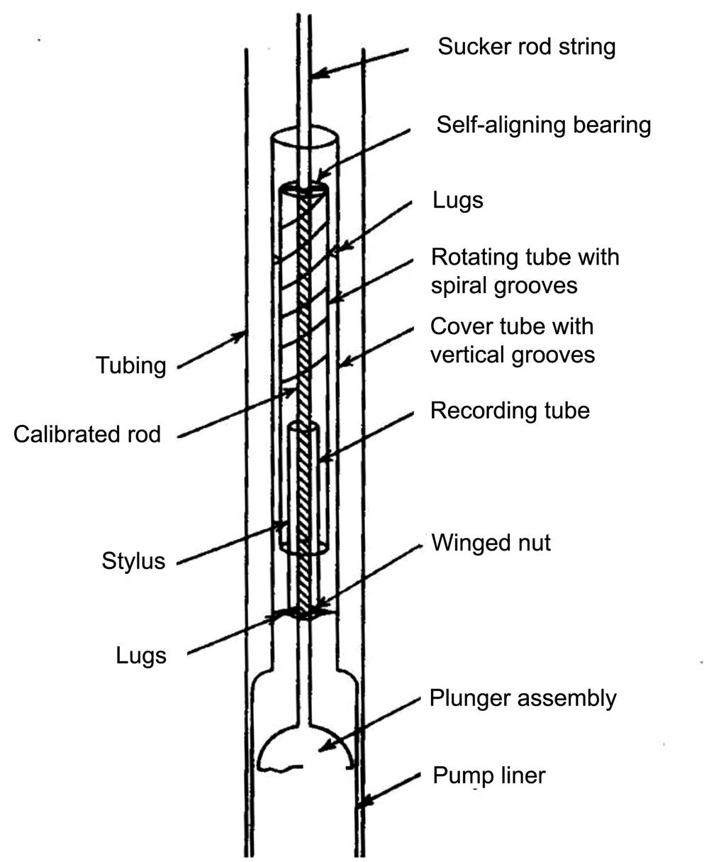
The relative motion between the cover tube (which is attached to the pump barrel and hence anchored to the tubing) and the calibrated rod (which is an integral part of the sucker rod string) is recorded as a horizontal line on the recording tube. This is achieved by having the recording tube mounted on a winged nut threaded onto the calibrated rod and prevented from rotating by means of two lugs, which are attached to the winged nut, which run in vertical grooves in the cover tube. The stylus is mounted on a third tube, which is free to rotate and is connected by a self-aligning bearing to the upper end of the calibrated rod. Lugs attached to the cover tube run in spiral grooves cut in the outer surface of the rotating tube. Consequently, vertical motion of the plunger assembly relative to the barrel results in rotation of the third tube, and the stylus cuts a horizontal line on a recording tube.
Any change in plunger loading causes a change in length of the section of the calibrated rod between the winged nut supporting the recording tube and the self-aligning bearing supporting the rotating tube (so that a vertical line is cut on the recording tube by the stylus). When the pump is in operation, the stylus traces a series of cards, one on top of the other. To obtain a new series of cards, the polished rod at the well head is rotated. This rotation is transmitted to the plunger in a few pump strokes. Because the recording tube is prevented from rotating by the winged nut lugs that run in the cover tube grooves, the rotation of the sucker rod string causes the winged nut to travel—upward or downward depending on the direction of rotation—on the threaded calibrated rod. Upon the completion of a series of tests, the recording tube (which is 36 in. long) is removed.
It is important to note that although the bottom-hole dynagraph records the plunger stroke and variations in plunger loading, no zero line is obtained. Thus, quantitative interpretation of the cards becomes somewhat speculative unless a pressure element is run with the dynagraph.
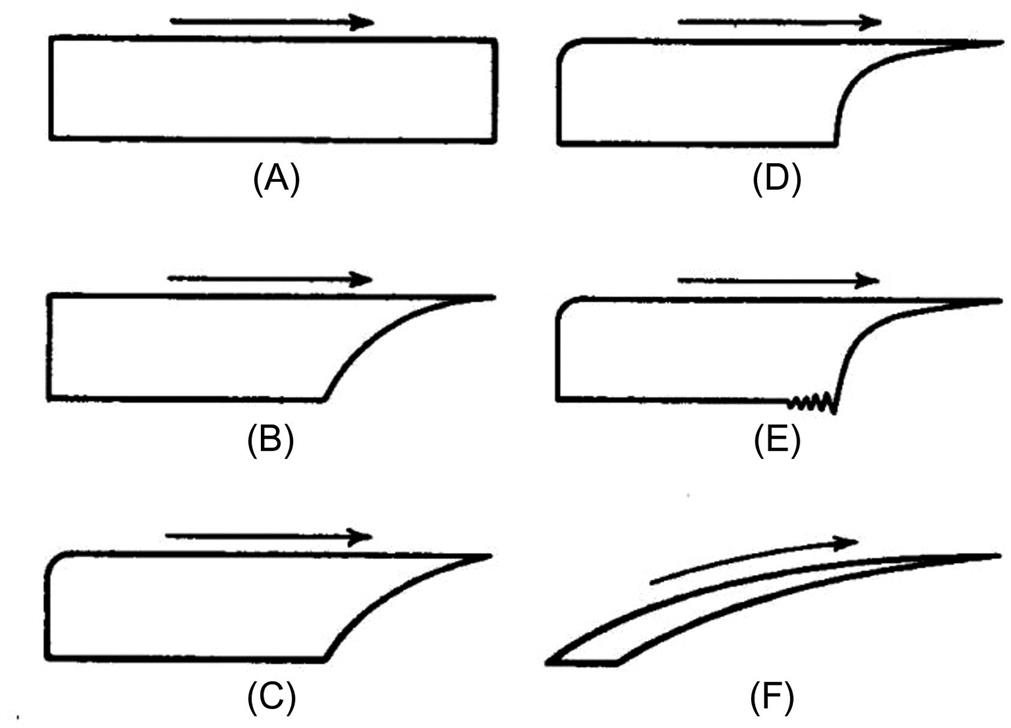
Fig. 16.10 shows some typical dynagraph card results. Card (A) shows an ideal case where instantaneous valve actions at the top and bottom of the stroke are indicated. In general, however, some free gas is drawn into the pump on the upstroke, so a period of gas compression can occur on the down-stroke before the TV opens. This is shown in card (B). Card (C) shows gas expansion during the upstroke giving a rounding of the card just as the upstroke begins. Card (D) shows fluid pounding that occurs when the well is almost pumped off (the pump displacement rate is higher than the formation of potential liquid production rate). This fluid pounding results in a rapid fall off in stress in the rod string and the sudden imposed shock to the system. Card (E) shows that the fluid pounding has progressed so that the mechanical shock causes oscillations in the system. Card (F) shows that the pump is operating at a very low volumetric efficiency where almost all the pump stroke is being lost in gas compression and expansion (no liquid is being pumped). This results in no valve action and the area between the card nearly disappears (thus, is gas locked). Usually, this gas-locked condition is only temporary, and as liquid leaks past the plunger, the volume of liquid in the pump barrel increases until the TV opens and pumping recommences.
The use of the pump dynagraph involves pulling the rods and pump from the well bath to install the instrument and to recover the recording tube. Also, the dynagraph cannot be used in a well that is equipped with a tubing pump. Thus, the dynagraph is more a research instrument than an operational device. Once there is knowledge from a dynagraph, surface dynamometer cards can be interpreted.
The surface, or polished rod, dynamometer is a device that records the motion (and its history) of the polished rod during the pumping cycle. The rod string is forced by the pumping unit to follow a regular time versus position pattern. However, the polished rod reacts with the loadings (on the rod string) that are imposed by the well.
The surface dynamometer cards record the history of the variations in loading on the polished rod during a cycle. The cards have three principal uses:
1. To obtain information that can be used to determine load, torque, and horsepower changes required of the pump equipment
2. To improve pump operating conditions such as pump speed and stroke length
3. To check well conditions after installation of equipment to prevent or diagnose various operating problems (like pounding, etc.)
Surface instruments can be mechanical, hydraulic, and electrical. One of the most common mechanical instruments is a ring dynamometer installed between the hanger bar and the polished rod clamp in such a manner as the ring may carry the entire well load. The deflection of the ring is proportional to the load, and this deflection is amplified and transmitted to the recording arm by a series of levers. A stylus on the recording arm traces a record of the imposed loads on a waxed (or via an ink pen) paper card located on a drum. The loads are obtained in terms of polished rod displacements by having the drum oscillate back and forth to reflect the polished rod motion. Correct interpretation of surface dynamometer card leads to estimate of various parameter values.
• Maximum and minimum PRLs can be read directly from the surface card (with the use of instrument calibration). These data then allow for the determination of the torque, counterbalance, and horsepower requirements for the surface unit.
• Rod stretch and contraction is shown on the surface dynamometer card. This phenomenon is reflected in the surface unit dynamometer card and is shown in Fig. 16.11A for an ideal case.
• Acceleration forces cause the ideal card to rotate clockwise. The PRL is higher at the bottom of the stroke and lower at the top of the stroke. Thus, in Fig. 16.11B, Point A is at the bottom of the stroke.
• Rod vibration causes a serious complication in the interpretation of the surface card. This is result of the closing of the TV and the “pickup” of the fluid load by the rod string. This is, of course, the fluid pounding. This phenomenon sets up damped oscillation (longitudinal and bending) in the rod string. These oscillations result in waves moving from one end of the rod string to the other. Because the polished rod moves slower near the top and bottom of the strokes, these stress (or load) fluctuations due to vibrations tend to show up more prominently at those locations on the cards. Fig. 16.11C shows typical dynamometer card with vibrations of the rod string.
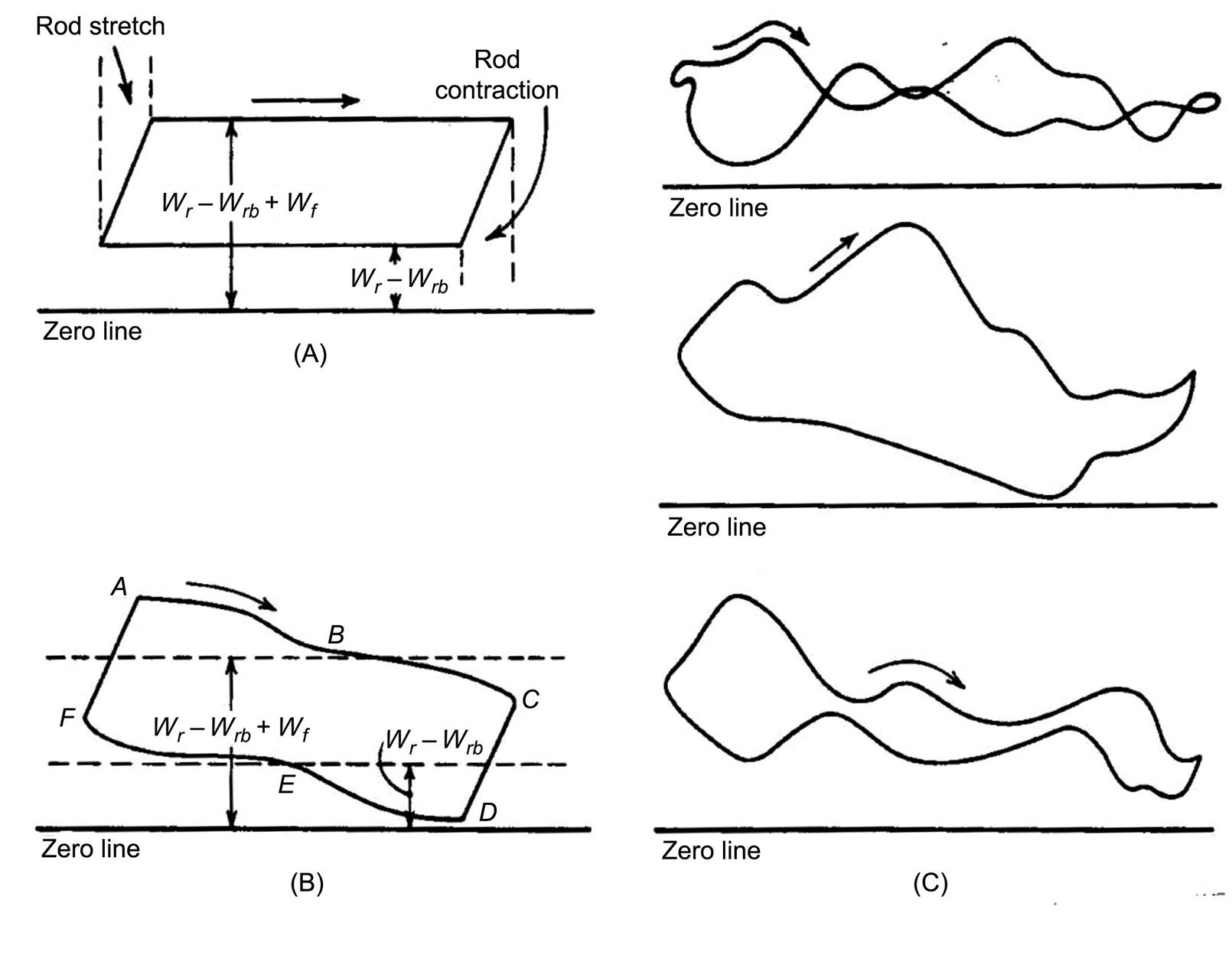
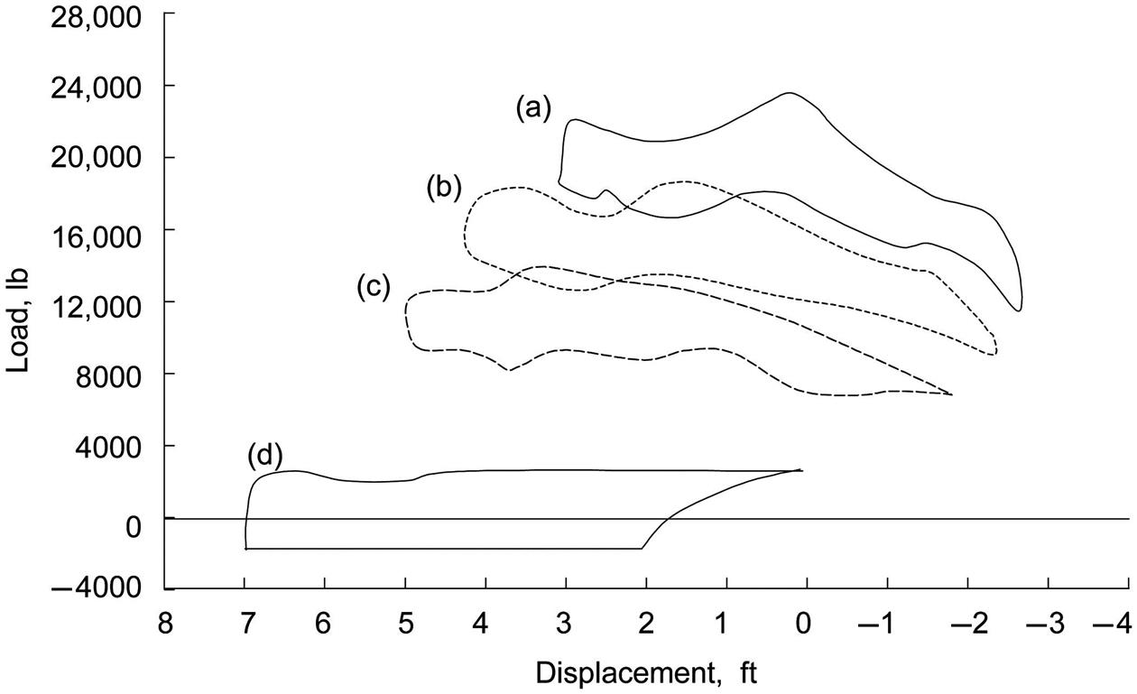
Fig. 16.12 presents a typical chart from a strain-gage type of dynamometer measured for a conventional unit operated with a 74-in. stroke at 15.4 strokes per minute. It shows the history of the load on the polished rod as a function of time (this is for a well 825 ft in depth with a No. 86 three-tapered rod string). Fig. 16.13 reproduces the data in Fig. 16.12 in a load versus displacement diagram. In the surface chart, we can see the peak load of 22,649 lb (which is 28,800 psi at the top of the 1-in. rod) in Fig. 16.13a. In Fig. 16.13b, we see the peak load of 17,800 lb (which is 29,600 psi at the top of the ⅞ -in. rod). In Fig. 16.13c, we see the peak load of 13,400 lb (which is 30,300 psi at the top of the ¾ -in. rod). In Fig. 16.13d is the dynagraph card at the plunger itself. This card indicates gross pump stroke of 7.1 ft, a net liquid stroke of 4.6 ft, and a fluid load of Wf=3200 lb. The shape of the pump card, Fig. 16.13d, indicates some down-hole gas compression. The shape also indicates that the tubing anchor is holding properly. A liquid displacement rate of 200 bbl/day is calculated and, compared to the surface measured production of 184 bbl/day, indicated no serious tubing flowing leak. The negative in Fig. 16.13d is the buoyancy of the rod string.

The information derived from the dynamometer card (dynagraph) can be used for evaluation of pump performance and troubleshooting of pumping systems. This subject is thoroughly addressed by Brown (1980).
16.8 Summary
This chapter presents the principles of sucker rod pumping systems and illustrates a procedure for selecting components of rod pumping systems. Major tasks include calculations of PRL, peak torque, stresses in the rod string, pump deliverability, and counterweight placement.
Problems
16.1. If the dimensions d1, d2, and c take the same values for both conventional unit (Class I lever system) and air-balanced unit (Class III lever system), how different will their polished rod strokes length be?
16.2. What are the advantages of the Lufkin Mark II and air-balanced units in comparison with conventional units?
16.3. Use your knowledge of kinematics to prove that for Class I lever systems,
a. the polished rod will travel faster in down stroke than in upstroke if the distance between crankshaft and the center of Sampson post is less than dimension d1.
b. the polished rod will travel faster in upstroke than in down stroke if the distance between crankshaft and the center of Sampson post is greater than dimension d1.
16.4. Derive a formula for calculating the effective diameter of a tapered rod string.
16.5. Derive formulas for calculating length fractions of equal-top-rod-stress tapered rod strings for (1) two-sized rod strings, (2) three-sized rod strings, and (3) four-sized rod strings. Plot size fractions for each case as a function of plunger area.
16.6. A tapered rod string consists of sections of ⅝- and ½- in. rods and a 2-in. plunger. Use the formulas from Problem 16.5 to calculate length fraction of each size of rod.
16.7. A tapered rod string consists of sections of ¾-, ⅝-, and ½-in. rods and a 1¾-in. plunger. Use the formulas from Problem 16.5 to calculate length fraction of each size of rod.
16.8. The following geometry dimensions are for the pumping unit C–80D–133–48:

Can this unit be used with a 2-in. plunger and ¾-in. rods to lift 30 °API gravity crude (formation volume factor 1.25 rb/stb) at depth of 2,000 ft? If yes, what is the required counterbalance load?
16.9. The following geometry dimensions are for the pumping unit C–320D–256–120:

Can this unit be used with a 2½-in. plunger and ¾-, ⅞-, 1-in. tapered rod string to lift 22° API gravity crude (formation volume factor 1.22 rb/stb) at a depth of 3000 ft? If yes, what is the required counterbalance load?
16.10. A well is pumped off with a rod pump described in Problem 16.8. A 2½-in. tubing string (2.875-in. OD, 2.441 ID) in the well is not anchored. Calculate (1) expected liquid production rate (use pump volumetric efficiency 0.80) and (2) required prime mover power (use safety factor 1.3).
16.11. A well is pumped with a rod pump described in Problem 16.9 to a liquid level of 2800 ft. A 3-in. tubing string (3½-in. OD, 2.995-in. ID) in the well is anchored. Calculate (1) expected liquid production rate (use pump volumetric efficiency 0.85) and (2) required prime mover power (use safety factor 1.4).
16.12. A well is to be put on a sucker rod pump. The proposed pump setting depth is 4500 ft. The anticipated production rate is 500 bbl/day oil of 40 °API gravity against wellhead pressure 150 psig. It is assumed that the working liquid level is low, and a sucker rod string having a working stress of 30,000 psi is to be used. Select surface and subsurface equipment for the installation. Use a safety factor of 1.40 for prime mover power.
16.13. A well is to be put on a sucker rod pump. The proposed pump setting depth is 4000 ft. The anticipated production rate is 550 bbl/day oil of 35 °API gravity against wellhead pressure 120 psig. It is assumed that working liquid level will be about 3000 ft, and a sucker rod string having a working stress of 30,000 psi is to be used. Select surface and subsurface equipment for the installation. Use a safety factor of 1.30 for prime mover power.