
Choke Performance
Abstract
Wellhead chokes are used to limit production rates for regulations, reduce liquid loading problems, avoid sand production problems due to high drawdown, and control flow rate to avoid water or gas coning. Two types of wellhead chokes are used: positive (fixed) chokes and adjustable chokes. Placing a choke at the wellhead means fixing the wellhead pressure and thus the flowing bottom-hole pressure and production rate. For a given wellhead pressure, the flowing bottom-hole pressure can be determined by calculating pressure loss in the tubing. If the reservoir pressure and productivity index are known, the flow rate can be determined on the basis of inflow performance relationship. This chapter presents and illustrates different mathematical models for describing choke performance.
Keywords
CPR; choke; sonic; subsonic; flow
5.1 Introduction
Wellhead chokes are used to limit production rates for regulations, protect surface equipment from slugging, avoid sand problems due to high drawdown, and control flow rate to avoid water or gas coning. Two types of wellhead chokes are used. They are (1) positive (fixed) chokes and (2) adjustable chokes.
Placing a choke at the wellhead means fixing the wellhead pressure and, thus, the flowing bottom-hole pressure and production rate. For a given wellhead pressure, by calculating pressure loss in the tubing the flowing bottom-hole pressure can be determined. If the reservoir pressure and productivity index is known, the flow rate can then be determined on the basis of inflow performance relationship (IPR).
5.2 Sonic and Subsonic Flow
Pressure drop across well chokes is usually very significant. There is no universal equation for predicting pressure drop across the chokes for all types of production fluids. Different choke flow models are available from the literature, and they have to be chosen based on the gas fraction in the fluid and flow regimes, that is, subsonic or sonic flow.
Both sound waves and pressure waves are mechanical waves. When the fluid flow velocity in a choke reaches the traveling velocity of sound in the fluid under the in-situ condition, the flow is called “sonic flow.” Under sonic flow conditions, the pressure wave downstream of the choke cannot go upstream through the choke because the medium (fluid) is traveling in the opposite direction at the same velocity. Therefore, a pressure discontinuity exists at the choke, that is, the downstream pressure does not affect the upstream pressure. Because of the pressure discontinuity at the choke, any change in the downstream pressure cannot be detected from the upstream pressure gauge. Of course, any change in the upstream pressure cannot be detected from the downstream pressure gauge either. This sonic flow provides a unique choke feature that stabilizes well production rate and separation operation conditions.
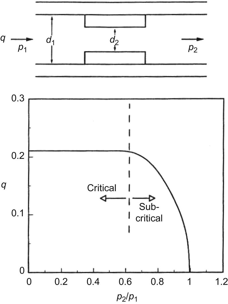
Whether a sonic flow exists at a choke depends on a downstream-to-upstream pressure ratio. If this pressure ratio is less than a critical pressure ratio, sonic (critical) flow exists. If this pressure ratio is greater than or equal to the critical pressure ratio, subsonic (subcritical) flow exists. The critical pressure ratio through chokes is expressed as
(5.1)
where poutlet is the pressure at choke outlet, pup is the upstream pressure, and k=Cp/Cv is the specific heat ratio. The value of the k is about 1.28 for natural gas. Thus, the critical pressure ratio is about 0.55 for natural gas. A similar constant is used for oil flow. A typical choke performance curve is shown in Fig. 5.1.
5.3 Single-Phase Liquid Flow
The pressure drop across a choke is mainly due to kinetic energy change. For single-phase liquid flow, the second term in the right-hand side of Eq. (4.1) can be rearranged as
(5.2)
If U.S. field units are used, Eq. (5.2) is expressed as
(5.3)
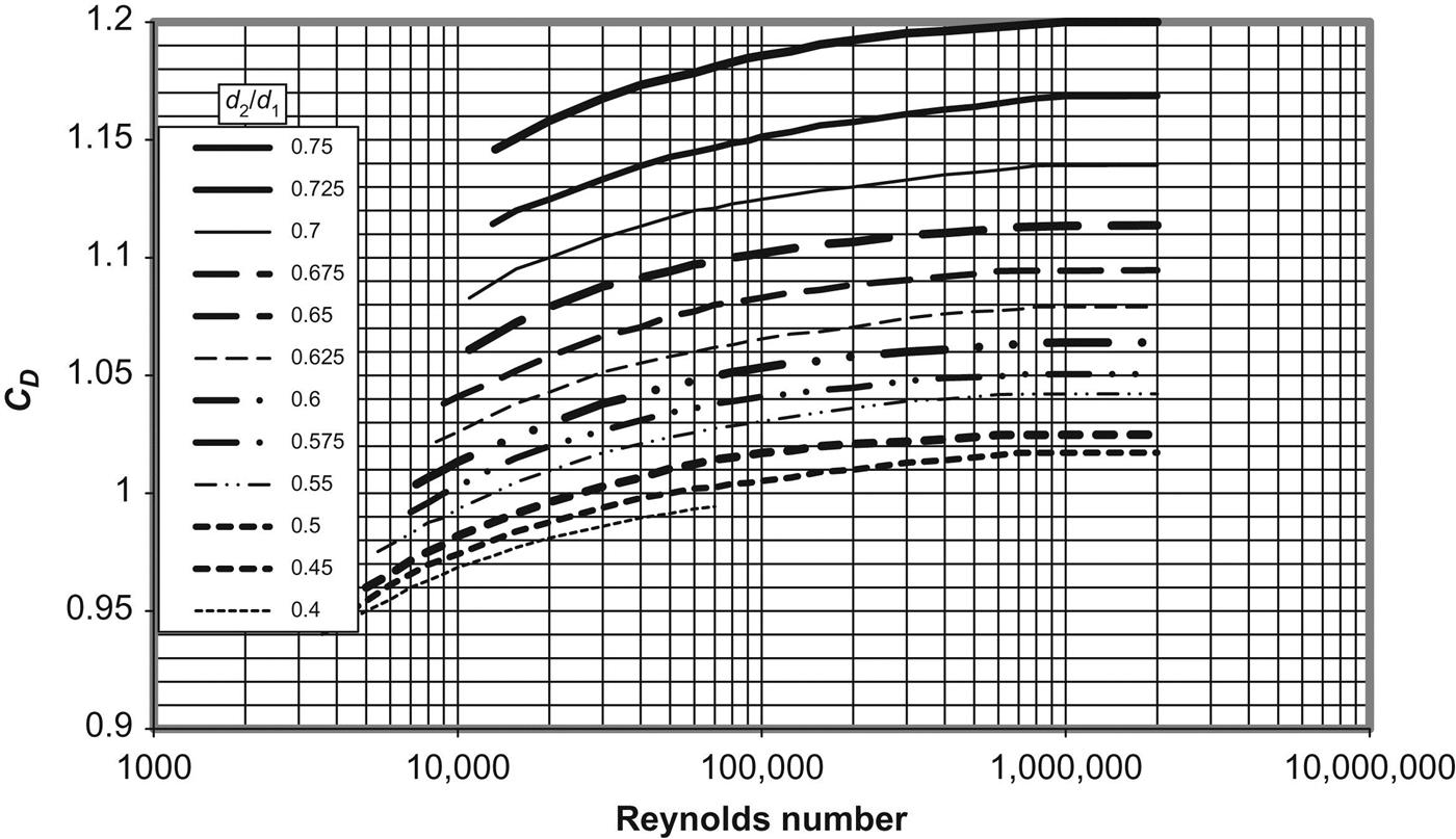
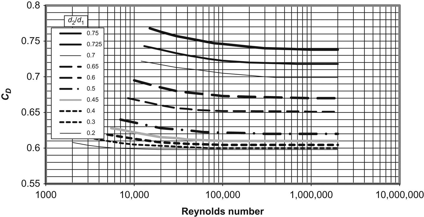
The choke discharge coefficient CD can be determined based on Reynolds number and choke/pipe diameter ratio (Figs. 5.2 and 5.3). The following correlation has been found to give reasonable accuracy for Reynolds numbers between 104 and 106 for nozzle-type chokes (Guo and Ghalambor, 2005):
(5.4)
 (5.4)
(5.4)
5.4 Single-Phase Gas Flow
Pressure equations for gas flow through a choke are derived based on an isentropic process. This is because there is no time for heat to transfer (adiabatic) and the friction loss is negligible (assuming reversible) at chokes. In addition to the concern of pressure drop across the chokes, temperature drop associated with choke flow is also an important issue for gas wells, because hydrates may form that may plug flow lines.
5.4.1 Subsonic Flow
Under subsonic flow conditions, gas passage through a choke can be expressed as
(5.5)
 (5.5)
(5.5)pup=upstream pressure at choke, psia
A2=cross-sectional area of choke, in.2
The Reynolds number for determining CD is expressed as
(5.6)
where μ is gas viscosity in cp.
Gas velocity under subsonic flow conditions is less than the sound velocity in the gas at the in-situ conditions:
(5.7)
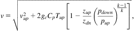 (5.7)
(5.7)where Cp=specific heat of gas at constant pressure (187.7 lbf-ft/lbm-R for air).
5.4.2 Sonic Flow
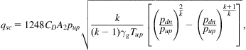
Under sonic flow conditions, the gas passage rate reaches its maximum value. The gas passage rate is expressed in the following equation for ideal gases:
(5.8)
 (5.8)
(5.8)The choke flow coefficient CD is not sensitive to the Reynolds number for Reynolds number values greater than 106. Thus, the CD value at the Reynolds number of 106 can be assumed for CD values at higher Reynolds numbers.
Gas velocity under sonic flow conditions is equal to sound velocity in the gas under the in-situ conditions:
(5.9)
or
(5.10)
5.4.3 Temperature at Choke
Depending on the upstream-to-downstream pressure ratio, the temperature at choke can be much lower than expected. This low temperature is due to the Joule–Thomson cooling effect, that is, a sudden gas expansion below the nozzle causes a significant temperature drop. The temperature can easily drop to below ice point, resulting in ice-plugging if water exists. Even though the temperature still can be above ice point, hydrates can form and cause plugging problems. Assuming an isentropic process for gas flowing through chokes, the temperature at the choke downstream can be predicted using the following equation:
(5.11)
The outlet pressure is equal to the downstream pressure in subsonic flow conditions.
5.4.4 Applications
Eqs. (5.5) through (5.11) can be used for estimating
• Gas passage rate at given upstream and downstream pressures
• Upstream pressure at given downstream pressure and gas passage
• Downstream pressure at given upstream pressure and gas passage
To estimate the gas passage rate at given upstream and downstream pressures, the following procedure can be taken:
Step 1. Calculate the critical pressure ratio with Eq. (5.1).
Step 2. Calculate the downstream-to-upstream pressure ratio.
Step 3. If the downstream-to-upstream pressure ratio is greater than the critical pressure ratio, use Eq. (5.5) to calculate gas passage. Otherwise, use Eq. (5.8) to calculate gas passage.
Example Problem 5.1 A 0.6 specific gravity gas flows from a 2-in. pipe through a 1-in. orifice-type choke. The upstream pressure and temperature are 800 psia and 75°F, respectively. The downstream pressure is 200 psia (measured 2 ft from the orifice). The gas-specific heat ratio is 1.3. (1) What is the expected daily flow rate? (2) Does heating need to be applied to ensure that the frost does not clog the orifice? (3) What is the expected pressure at the orifice outlet?

Assuming NRe>106, Fig. 5.2 gives CD=0.62.
μ=0.01245 cp by the Carr–Kobayashi–Burrows correlation.
Therefore, heating is needed to prevent icing.
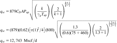
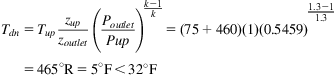
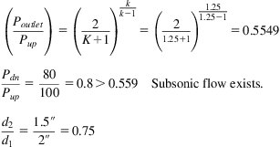
Example Problem 5.2 A 0.65 specific gravity natural gas flows from a 2-in. pipe through a 1.5-in. nozzle-type choke. The upstream pressure and temperature are 100 psia and 70°F, respectively. The downstream pressure is 80 psia (measured 2 ft from the nozzle). The gas-specific heat ratio is 1.25. (1) What is the expected daily flow rate? (2) Is icing a potential problem? (3) What is the expected pressure at the nozzle outlet?
Assuming NRe>106, Fig. 5.1 gives CD=1.2.

μ=0.0108 cp by the Carr–Kobayashi–Burrows correlation.

Heating may not be needed, but the hydrate curve may need to be checked.
for subcritical flow.
To estimate upstream pressure at a given downstream pressure and gas passage, the following procedure can be taken:
Step 1. Calculate the critical pressure ratio with Eq. (5.1).
Step 2. Calculate the minimum upstream pressure required for sonic flow by dividing the downstream pressure by the critical pressure ratio.
Step 3. Calculate gas flow rate at the minimum sonic flow condition with Eq. (5.8).
Step 4. If the given gas passage is less than the calculated gas flow rate at the minimum sonic flow condition, use Eq. (5.5) to solve upstream pressure numerically. Otherwise, Eq. (5.8) to calculate upstream pressure.
Example Problem 5.3 For the following given data, estimate upstream pressure at choke:
| Downstream pressure: | 300 psia |
| Choke size: | 32 1/64 in. |
| Flowline ID: | 2 in. |
| Gas production rate: | 5000 Mscf/d |
| Gas-specific gravity: | 0.75 1 for air |
| Gas-specific heat ratio: | 1.3 |
| Upstream temperature: | 110°F |
| Choke discharge coefficient: | 0.99 |
Solution Example Problem 5.3 is solved with the spreadsheet program GasUpChokePressure.xls. The result is shown in Table 5.1.
Table 5.1
Solution Given by the Spreadsheet Program GasUpChokePressure.xls
| GasUpChokePressure.xls | |
| Description: This spreadsheet calculates upstream pressure at choke for dry gases. | |
| Instructions: (1) Update parameter values in blue; (2) click Solution button; (3) view results. | |
| Input Data | |
| Downstream pressure: | 300 psia |
| Choke size: | |
| Flowline ID: | 2 in. |
| Gas production rate: | 5000 Mscf/d |
| Gas-specific gravity: | 0.75 1 for air |
| Gas-specific heat ratio (k): | 1.3 |
| Upstream temperature: | 110°F |
| Choke discharge coefficient: | 0.99 |
| Solution | |
| Choke area: | 0.19625 in.2 |
| Critical pressure ratio: | 0.5457 |
| Minimum upstream pressure required for sonic flow: | 549.72 psia |
| Flow rate at the minimum sonic flow condition: | 3029.76 Mscf/d |
| Flow regime (1=sonic flow; −1=subsonic flow): | 1 |
| Upstream pressure given by sonic flow equation: | 907.21 psia |
| Upstream pressure given by subsonic flow equation: | 1088.04 psia |
| Estimated upstream pressure: | 907.21 psia |

Downstream pressure cannot be calculated on the basis of given upstream pressure and gas passage under sonic flow conditions, but it can be calculated under subsonic flow conditions. The following procedure can be followed:
Step 1. Calculate the critical pressure ratio with Eq. (5.1).
Step 2. Calculate the maximum downstream pressure for minimum sonic flow by multiplying the upstream pressure by the critical pressure ratio.
Step 3. Calculate gas flow rate at the minimum sonic flow condition with Eq. (5.8).
Step 4. If the given gas passage is less than the calculated gas flow rate at the minimum sonic flow condition, use Eq. (5.5) to solve downstream pressure numerically. Otherwise, the downstream pressure cannot be calculated. The maximum possible downstream pressure for sonic flow can be estimated by multiplying the upstream pressure by the critical pressure ratio.
Example Problem 5.4 For the following given data, estimate downstream pressure at choke:
| Upstream pressure: | 600 psia |
| Choke size: | 32 1/64 in. |
| Flowline ID: | 2 in. |
| Gas production rate: | 2500 Mscf/d |
| Gas-specific gravity: | 0.75 1 for air |
| Gas-specific heat ratio: | 1.3 |
| Upstream temperature: | 110°F |
| Choke discharge coefficient: | 0.99 |
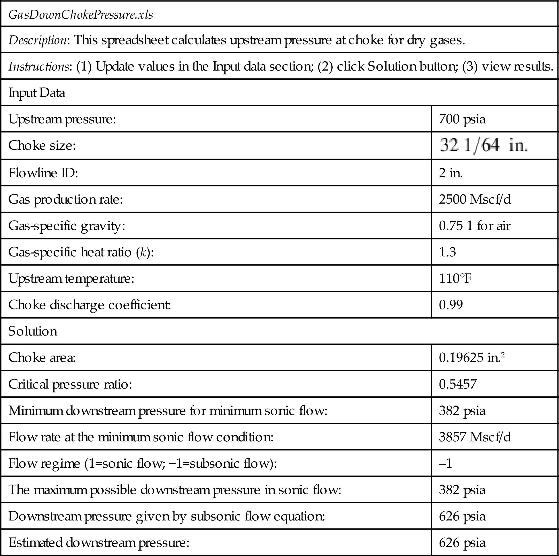
Solution Example Problem 5.4 is solved with the spreadsheet program GasDownChokePressure.xls. The result is shown in Table 5.2.
Table 5.2
Solution Given by the Spreadsheet Program GasDownChokePressure.xls
| GasDownChokePressure.xls | |
| Description: This spreadsheet calculates upstream pressure at choke for dry gases. | |
| Instructions: (1) Update values in the Input data section; (2) click Solution button; (3) view results. | |
| Input Data | |
| Upstream pressure: | 700 psia |
| Choke size: | |
| Flowline ID: | 2 in. |
| Gas production rate: | 2500 Mscf/d |
| Gas-specific gravity: | 0.75 1 for air |
| Gas-specific heat ratio (k): | 1.3 |
| Upstream temperature: | 110°F |
| Choke discharge coefficient: | 0.99 |
| Solution | |
| Choke area: | 0.19625 in.2 |
| Critical pressure ratio: | 0.5457 |
| Minimum downstream pressure for minimum sonic flow: | 382 psia |
| Flow rate at the minimum sonic flow condition: | 3857 Mscf/d |
| Flow regime (1=sonic flow; −1=subsonic flow): | –1 |
| The maximum possible downstream pressure in sonic flow: | 382 psia |
| Downstream pressure given by subsonic flow equation: | 626 psia |
| Estimated downstream pressure: | 626 psia |
5.5 Multiphase Flow
When the produced oil reaches the wellhead choke, the wellhead pressure is usually below the bubble-point pressure of the oil. This means that free gas exists in the fluid stream flowing through choke. Choke behaves differently depending on gas content and flow regime (sonic or subsonic flow).
5.5.1 Critical (Sonic) Flow
Tangren et al. (1947) performed the first investigation on gas-liquid two-phase flow through restrictions. They presented an analysis of the behavior of an expanding gas-liquid system. They showed that when gas bubbles are added to an incompressible fluid, above a critical flow velocity, the medium becomes incapable of transmitting pressure change upstream against the flow. Several empirical choke flow models have been developed in the past half century. They generally take the following form for sonic flow:
(5.12)
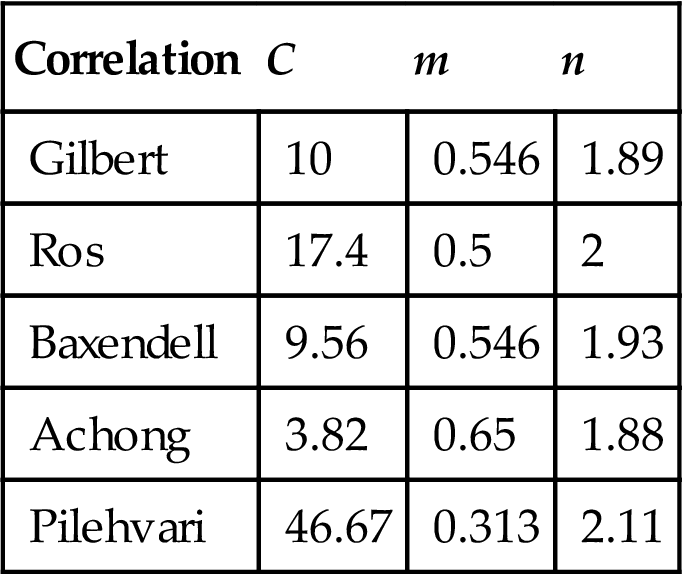
and C, m, and n are empirical constants related to fluid properties. On the basis of the production data from Ten Section Field in California, Gilbert (1954) found the values for C, m, and n to be 10, 0.546, and 1.89, respectively. Other values for the constants were proposed by different researchers including Baxendell (1957), Ros (1960), Achong (1961), and Pilehvari (1980). A summary of these values is presented in Table 5.3. Poettmann and Beck (1963) extended the work of Ros (1960) to develop charts for different API crude oils. Omana et al. (1969) derived dimensionless choke correlations for water-gas systems.
5.5.2 Subcriticai (Subsonic) Flow
Mathematical modeling of subsonic flow of multiphase fluid through choke has been controversial over decades. Fortunati (1972) was the first investigator who presented a model that can be used to calculate critical and subcritical two-phase flow through chokes. Ashford (1974) also developed a relation for two-phase critical flow based on the work of Ros (1960). Gould (1974) plotted the critical–subcritical boundary defined by Ashford, showing that different values of the polytropic exponents yield different boundaries. Ashford and Pierce (1975) derived an equation to predict the critical pressure ratio. Their model assumes that the derivative of flow rate with respect to the downstream pressure is zero at critical conditions. One set of equations was recommended for both critical and subcritical flow conditions. Pilehvari (1980, 1981) also studied choke flow under subcritical conditions. Sachdeva et al. (1986) extended the work of Ashford and Pierce (1975) and proposed a relationship to predict critical pressure ratio. He also derived an expression to find the boundary between critical and subcritical flow. Surbey et al. (1988, 1989) discussed the application of multiple orifice valve chokes for both critical and subcritical flow conditions. Empirical relations were developed for gas and water systems. Al-Attar and Abdul-Majeed (1988) made a comparison of existing choke flow models. The comparison was based on data from 155 well tests. They indicated that the best overall comparison was obtained with the Gilbert correlation, which predicted measured production rate within an average error of 6.19%. On the basis of energy equation, Perkins (1990) derived equations that describe isentropic flow of multiphase mixtures through chokes. Osman and Dokla (1990) applied the least-square method to field data to develop empirical correlations for gas condensate choke flow. Gilbert-type relationships were generated. Applications of these choke flow models can be found elsewhere (Wallis, 1969; Perry, 1973; Brown and Beggs, 1977; Brill and Beggs, 1978; Ikoku, 1980; Nind, 1981; Bradley, 1987; Beggs, 1991; Saberi, 1996).
Sachdeva’s multiphase choke flow mode is representative of most of these works and has been coded in some commercial network modeling software. This model uses the following equation to calculate the critical–subcritical boundary:
(5.13)
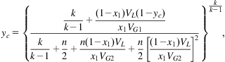 (5.13)
x1=free gas quality at upstream, mass fraction
VL=liquid-specific volume at upstream, ft3/lbm
The polytropic exponent for gas is calculated using
(5.14)
The gas-specific volume at upstream (VG1) can be determined using the gas law based on upstream pressure and temperature. The gas-specific volume at downstream (VG2) is expressed as
(5.15)
The critical pressure ratio yc can be solved from Eq. (5.13) numerically.
The actual pressure ratio can be calculated by
(5.16)
If ya<yc, critical flow exists, and the yc should be used (y=yc). Otherwise, subcritical flow exists, and ya should be used (y=ya).
The total mass flux can be calculated using the following equation:
(5.17)
G2=mass flux at downstream, lbm/ft2/s
CD=discharge coefficient, 0.62–0.90
The mixture density at downstream (ρm2) can be calculated using the following equation:
(5.18)
Once the mass flux is determined from Eq. (5.17), mass flow rate can be calculated using the following equation:
(5.19)
Liquid mass flow rate is determined by
(5.20)
At typical velocities of mixtures of 50–150 ft/s flowing through chokes, there is virtually no time for mass transfer between phases at the throat. Thus, x2=x1 can be assumed. Liquid volumetric flow rate can then be determined based on liquid density.
Gas mass flow rate is determined by
(5.21)
Gas volumetric flow rate at choke downstream can then be determined using gas law based on downstream pressure and temperature.
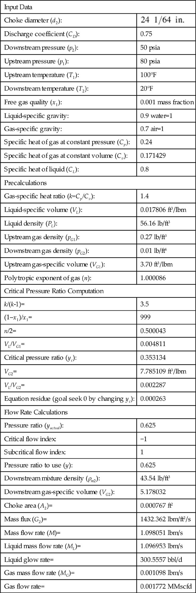
The major drawback of Sachdeva’s multiphase choke flow model is that it requires free gas quality as an input parameter to determine flow regime and flow rates, and this parameter is usually not known before flow rates are known. A trial-and-error approach is, therefore, needed in flow rate computations. Table 5.4 shows an example calculation with Sachdeva’s choke model. Guo et al. (2002) investigated the applicability of Sachdeva’s choke flow model in southwest Louisiana gas condensate wells. A total of 512 data sets from wells in southwest Louisiana were gathered for this study. Out of these data sets, 239 sets were collected from oil wells and 273 from condensate wells. Each of the data sets includes choke size, gas rate, oil rate, condensate rate, water rate, gas–liquid ratio, upstream and downstream pressures, oil API gravity, and gas deviation factor (z-factor). Liquid and gas flow rates from these wells were also calculated using Sachdeva’s choke model. The overall performance of the model was studied in predicting the gas flow rate from both oil and gas condensate wells. Out of the 512 data sets, 48 sets failed to comply with the model. Mathematical errors occurred in finding square roots of negative numbers. These data sets were from the condensate wells where liquid densities ranged from 46.7 to 55.1 lb/ft3 and recorded pressure differential across the choke less than 1100 psi. Therefore, only 239 data sets from oil wells and 235 sets from condensate wells were used. The total number of data sets is 474. Different values of discharge coefficient CD were used to improve the model performance. Based on the cases studied, Guo et al. (2002) draw the following conclusions:
1. The accuracy of Sachdeva’s choke model can be improved by using different discharge coefficients for different fluid types and well types.
2. For predicting liquid rates of oil wells and gas rates of gas condensate wells, a discharge coefficient of CD=1.08 should be used.
3. A discharge coefficient CD=0.78 should be used for predicting gas rates of oil wells.
4. A discharge coefficient CD=1.53 should be used for predicting liquid rates of gas condensate wells.
Table 5.4
An Example Calculation with Sachdeva’s Choke Model
| Input Data | |
| Choke diameter (d2): | |
| Discharge coefficient (CD): | 0.75 |
| Downstream pressure (p2): | 50 psia |
| Upstream pressure (p1): | 80 psia |
| Upstream temperature (T1): | 100°F |
| Downstream temperature (T2): | 20°F |
| Free gas quality (x1): | 0.001 mass fraction |
| Liquid-specific gravity: | 0.9 water=1 |
| Gas-specific gravity: | 0.7 air=1 |
| Specific heat of gas at constant pressure (Cp): | 0.24 |
| Specific heat of gas at constant volume (Cv): | 0.171429 |
| Specific heat of liquid (CL): | 0.8 |
| Precalculations | |
| Gas-specific heat ratio (k=Cp/Cv): | 1.4 |
| Liquid-specific volume (VL): | 0.017806 ft3/lbm |
| Liquid density (PL): | 56.16 lb/ft3 |
| Upstream gas density (pG1): | 0.27 lb/ft3 |
| Downstream gas density (pG2): | 0.01 lb/ft4 |
| Upstream gas-specific volume (VG1): | 3.70 ft3/lbm |
| Polytropic exponent of gas (n): | 1.000086 |
| Critical Pressure Ratio Computation | |
| k/(k-1)= | 3.5 |
| (1–x1)/x1= | 999 |
| n/2= | 0.500043 |
| VL/VG1= | 0.004811 |
| Critical pressure ratio (yc): | 0.353134 |
| VG2= | 7.785109 ft3/lbm |
| VL/VG2= | 0.002287 |
| Equation residue (goal seek 0 by changing yc): | 0.000263 |
| Flow Rate Calculations | |
| Pressure ratio (yactual): | 0.625 |
| Critical flow index: | −1 |
| Subcritical flow index: | 1 |
| Pressure ratio to use (y): | 0.625 |
| Downstream mixture density (ρm2): | 43.54 lb/ft3 |
| Downstream gas-specific volume (VG2): | 5.178032 |
| Choke area (A2)= | 0.000767 ft2 |
| Mass flux (G2)= | 1432.362 lbm/ft2/s |
| Mass flow rate (M)= | 1.098051 lbm/s |
| Liquid mass flow rate (ML)= | 1.096953 lbm/s |
| Liquid glow rate= | 300.5557 bbl/d |
| Gas mass flow rate (MG)= | 0.001098 lbm/s |
| Gas flow rate= | 0.001772 MMscfd |
5.6 Summary
This chapter presented and illustrated different mathematical models for describing choke performance. While the choke models for gas flow have been well established with fairly good accuracy in general, the models for two-phase flow are subject to tuning to local oil properties. It is essential to validate two-phase flow choke models before they are used on a large scale.
Problems
5.1. A well is producing 40 °API oil at 200 stb/d and no gas. If the beam size is 1 in., pipe size is 2 in., temperature is 100°F, estimate pressure drop across a nozzle-type choke.
5.2. A well is producing at 200 stb/d of liquid along with a 900 scf/stb of gas. If the beam size is ½ in., assuming sonic flow, calculate the flowing wellhead pressure using Gilbert’s formula.
5.3. A 0.65 specific gravity gas flows from a 2-in. pipe through a 1-in. orifice-type choke. The upstream pressure and temperature are 850 psia and 85°F, respectively. The downstream pressure is 210 psia (measured 2 ft from the orifice). The gas-specific heat ratio is 1.3. (1) What is the expected daily flow rate? (2) Does heating need to be applied to ensure that the frost does not clog the orifice? (3) What is the expected pressure at the orifice outlet?
5.4. A 0.70 specific gravity natural gas flows from a 2-in. pipe through a 1.5-in. nozzle-type choke. The upstream pressure and temperature are 120 psia and 75°F, respectively. The downstream pressure is 90 psia (measured 2 ft from the nozzle). The gas-specific heat ratio is 1.25. (1) What is the expected daily flow rate? (2) Is icing a potential problem? (3) What is the expected pressure at the nozzle outlet?
5.5. For the following given data, estimate upstream gas pressure at choke:
| Downstream pressure: | 350 psia |
| Choke size: | 32 1/64 in. |
| Flowline ID: | 2 in. |
| Gas production rate: | 4000 Mscf/d |
| Gas-specific gravity: | 0.70 1 for air |
| Gas-specific heat ratio: | 1.25 |
| Upstream temperature: | 100°F |
| Choke discharge coefficient: | 0.95 |
5.6. For the following given data, estimate downstream gas pressure at choke:
| Upstream pressure: | 620 psia |
| Choke size: | 32 1/64 in. |
| Flowline ID: | 2 in. |
| Gas production rate: | 2200 Mscf/d |
| Gas-specific gravity: | 0.65 1 for air |
| Gas-specific heat ratio: | 1.3 |
| Upstream temperature: | 120°F |
| Choke discharge coefficient: | 0.96 |
5.7. For the following given data, assuming subsonic flow, estimate liquid and gas production rate:
| Choke diameter: | 32 1/64 in. |
| Discharge coefficient: | 0.85 |
| Downstream pressure: | 60 psia |
| Upstream pressure: | 90 psia |
| Upstream temperature: | 120°F |
| Downstream temperature: | 30°F |
| Free gas quality: | 0.001 mass fraction |
| Liquid-specific gravity: | 0.85 water=1 |
| Gas-specific gravity: | 0.75 air=1 |
| Specific heat of gas at constant pressure: | 0.24 |
| Specific heat of gas at constant volume: | 0.171429 |
| Specific heat of liquid: | 0.8 |