
• Flowlines transporting oil and/or gas from satellite wells to manifolds
• Flowlines transporting oil and/or gas from manifolds to production facility
• Infield flowlines transporting oil and/or gas from between production facilities
• Export pipelines transporting oil and/or gas from production facilities to refineries/users
The pipelines are sized to handle the expected pressure and fluid flow on the basis of flow assurance analysis. This section covers the following topics:
11.4.1 Flow in Pipelines
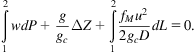
Designing a long-distance pipeline for transportation of crude oil and natural gas requires knowledge of flow formulas for calculating capacity and pressure requirements. Based on the first law of thermal dynamics, the total pressure gradient is made up of three distinct components:
(11.78)
where
![]() =pressure gradient due to elevation or potential energy change
=pressure gradient due to elevation or potential energy change
![]() =pressure gradient due to frictional losses
=pressure gradient due to frictional losses
![]() =pressure gradient due to acceleration or kinetic energy change
=pressure gradient due to acceleration or kinetic energy change
g=gravitational acceleration, ft/sec2
θ=dip angle from horizontal direction, °
The elevation component is pipe-angle dependent. It is zero for horizontal flow. The friction loss component applies to any type of flow at any pipe angle and causes a pressure drop in the direction of flow. The acceleration component causes a pressure drop in the direction of velocity increase in any flow condition in which velocity changes occurs. It is zero for constant-area, incompressible flow. This term is normally negligible for both oil and gas pipelines.
The friction factor fM in Eq. (11.78) can be determined based on flow regimes, that is, laminar flow or turbulent flow. Reynolds number (NRe) is used as a parameter to distinguish between laminar and turbulent fluid flow. Reynolds number is defined as the ratio of fluid momentum force to viscous shear force. The Reynolds number can be expressed as a dimensionless group defined as
(11.79)
The change from laminar to turbulent flow is usually assumed to occur at a Reynolds number of 2100 for flow in a circular pipe. If U.S. field units of ft for diameter, ft/sec for velocity, lbm/ft3 for density and centipoises for viscosity are used, the Reynolds number equation becomes
(11.80)
For a gas with specific gravity γg and viscosity μg (cp) flowing in a pipe with an inner diameter D (in.) at flow rate q (Mcfd) measured at base conditions of Tb (°R) and pb (psia), the Reynolds number can be expressed as
(11.81)
The Reynolds number usually takes values greater than 10,000 in gas pipelines. As Tb is 520°R and pb varies only from 14.4 to 15.025 psia in the United States, the value of 711pb/Tb varies between 19.69 and 20.54. For all practical purposes, the Reynolds number for natural gas flow problems may be expressed as
(11.82)
q=gas flow rate at 60°F and 14.73 psia, Mcfd
γg=gas-specific gravity (air=1)
The coefficient 20 becomes 0.48 if q is in scfh.
Fig. 11.10 is a friction factor chart covering the full range of flow conditions. It is a log-log graph of (log fM) versus (log NRe). Because of the complex nature of the curves, the equation for the friction factor in terms of the Reynolds number and relative roughness varies in different regions.
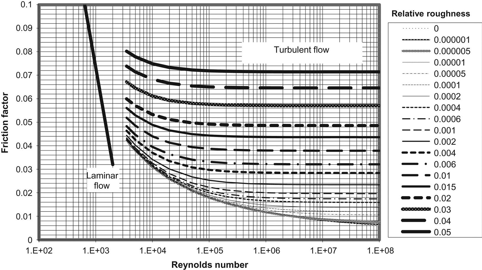
In the laminar flow region, the friction factor can be determined analytically. The Hagen–Poiseuille equation for laminar flow is
(11.83)
Equating the frictional pressure gradients given by Eqs. (11.78) and (11.83) gives
(11.84)
which yields
(11.85)
In the turbulent flow region, a number of empirical correlations for friction factors are available. Only the most accurate ones are presented in this section.
For smooth wall pipes in the turbulent flow region, Drew et al. (1930) presented the most commonly used correlation:
(11.86)
which is valid over a wide range of Reynolds numbers, 3×10³<NRe<3×10⁶.
For rough wall pipes in the turbulent flow region, the effect of wall roughness on friction factor depends on the relative roughness and Reynolds number. The Nikuradse (1933) friction factor correlation is still the best one available for fully developed turbulent flow in rough pipes:
(11.87)
This equation is valid for large values of the Reynolds number where the effect of relative roughness is dominant. The correlation that is used as the basis for modern friction factor charts was proposed by Colebrook (1983):
(11.88)
which is applicable to smooth pipes and to flow in transition and fully rough zones of turbulent flow. It degenerates to the Nikuradse correlation at large values of the Reynolds number. Eq. (11.88) is not explicit in fM. However, values of fM can be obtained by a numerical procedure such as Newton–Raphson iteration. An explicit correlation for friction factor was presented by Jain (1976):
(11.89)
This correlation is comparable to the Colebrook correlation. For relative roughness between 10−6 and 10−2 and the Reynolds number between 5×10³ and 108, the errors were reported to be within +1% when compared with the Colebrook correlation. Therefore, Eq. (11.89) is recommended for all calculations requiring friction factor determination of turbulent flow.
The wall roughness is a function of pipe material, method of manufacturing, and the environment to which it has been exposed. From a microscopic sense, wall roughness is not uniform, and thus, the distance from the peaks to valleys on the wall surface will vary greatly. The absolute roughness, ε, of a pipe wall is defined as the mean protruding height of relatively uniformly distributed and sized, tightly packed sand grains that would give the same pressure gradient behavior as the actual pipe wall. Analysis has suggested that the effect of roughness is not due to its absolute dimensions, but to its dimensions relative to the inside diameter of the pipe. Relative roughness, eD, is defined as the ratio of the absolute roughness to the pipe internal diameter:
(11.90)
where ε and D have the same unit.
The absolute roughness is not a directly measurable property for a pipe, which makes the selection of value of pipe wall roughness difficult. The way to evaluate the absolute roughness is to compare the pressure gradients obtained from the pipe of interest with a pipe that is sand roughened. If measured pressure gradients are available, the friction factor and Reynolds number can be calculated and an effective eD obtained from the Moody diagram. This value of eD should then be used for future predictions until updated. If no information is available on roughness, a value of ε=0.0006 in. is recommended for tubing and line pipes.
11.4.1.1 Oil flow
This section addresses flow of crude oil in pipelines. Flow of multiphase fluids is discussed in other literatures such as that of Guo et al. (2005).
Crude oil can be treated as an incompressible fluid. The relation between flow velocity and driving pressure differential for a given pipeline geometry and fluid properties is readily obtained by integration of Eq. (11.78) when the kinetic energy term is neglected:
(11.91)
which can be written in flow rate as
(11.92)
When changed to U.S. field units, Eq. (11.92) becomes
(11.93)
Example Problem 11.4 A 35 API gravity, 5 cp, oil is transported through a 6-in. (I.D.) pipeline with an uphill angle of 15° across a distance of 5 miles at a flow rate of 5000 bbl/day. Estimate the minimum required pump pressure to deliver oil at 50 psi pressure at the outlet. Assume e=0.0006 in.
Solution
Pipe inner area:
The average oil velocity in pipe:
Oil-specific gravity:
Reynolds number:

Eq. (11.89) gives
which gives
Eq. (11.93) gives

11.4.1.2 Gas flow
Consider steady-state flow of dry gas in a constant-diameter, horizontal pipeline. The mechanical energy equation, Eq. (11.78), becomes
(11.94)
which serves as a base for development of many pipeline equations. The difference in these equations originated from the methods used in handling the z-factor and friction factor. Integrating Eq. (11.94) gives
(11.95)
If temperature is assumed constant at average value in a pipeline, ![]() , and gas deviation factor,
, and gas deviation factor, ![]() , is evaluated at average temperature and average pressure,
, is evaluated at average temperature and average pressure, ![]() , Eq. (11.95) can be evaluated over a distance L between upstream pressure, p1, and downstream pressure, p2:
, Eq. (11.95) can be evaluated over a distance L between upstream pressure, p1, and downstream pressure, p2:
(11.96)
Eq. (11.96) may be written in terms of flow rate measured at arbitrary base conditions (Tb and pb):
(11.97)
where C is a constant with a numerical value that depends on the units used in the pipeline equation. If L is in miles and q is in scfd, C=77.54.
The use of Eq. (11.97) involves an iterative procedure. The gas deviation factor depends on pressure and the friction factor depends on flow rate. This problem prompted several investigators to develop pipeline flow equations that are noniterative or explicit. This has involved substitutions for the friction factor fM. The specific substitution used may be diameter-dependent only (Weymouth equation) or Reynolds number–dependent only (Panhandle equations).
11.4.1.2.1 Weymouth equation for horizontal flow
Eq. (11.97) takes the following form when the unit of scfh for gas flow rate is used:
(11.98)
where ![]() is called the “transmission factor.” The friction factor may be a function of flow rate and pipe roughness. If flow conditions are in the fully turbulent region, Eq. (11.89) degenerates to
is called the “transmission factor.” The friction factor may be a function of flow rate and pipe roughness. If flow conditions are in the fully turbulent region, Eq. (11.89) degenerates to
(11.99)
where fM depends only on the relative roughness, eD. When flow conditions are not completely turbulent, fM depends on the Reynolds number also.
Therefore, use of Eq. (11.98) requires a trial-and-error procedure to calculate qh. To eliminate the trial-and-error procedure, Weymouth proposed that f vary as a function of diameter as follows:
(11.100)
With this simplification, Eq. (11.98) reduces to
(11.101)
which is the form of the Weymouth equation commonly used in the natural gas industry.
The use of the Weymouth equation for an existing transmission line or for the design of a new transmission line involves a few assumptions including no mechanical work, steady-flow, isothermal flow, constant compressibility factor, horizontal flow, and no kinetic energy change. These assumptions can affect accuracy of calculation results.
In the study of an existing pipeline, the pressure-measuring stations should be placed so that no mechanical energy is added to the system between stations. No mechanical work is done on the fluid between the points at which the pressures are measured. Thus, the condition of no mechanical work can be fulfilled.
Steady flow in pipeline operation seldom, if ever, exists in actual practice because pulsations, liquid in the pipeline, and variations in input or output gas volumes cause deviations from steady-state conditions. Deviations from steady-state flow are the major cause of difficulties experienced in pipeline flow studies.
The heat of compression is usually dissipated into the ground along a pipeline within a few miles downstream from the compressor station. Otherwise, the temperature of the gas is very near that of the containing pipe, and because pipelines usually are buried, the temperature of the flowing gas is not influenced appreciably by rapid changes in atmospheric temperature. Therefore, the gas flow can be considered isothermal at an average effective temperature without causing significant error in long-pipeline calculations.
The compressibility of the fluid can be considered constant and an average effective gas deviation factor may be used. When the two pressures p1 and p2 lie in a region where z is essentially linear with pressure, it is accurate enough to evaluate ![]() at the average pressure
at the average pressure ![]() . One can also use the arithmetic average of the z's with
. One can also use the arithmetic average of the z's with ![]() , where z1 and z2 are obtained at p1 and p2, respectively. On the other hand, should p1 and p2 lie in the range where z is not linear with pressure (double-hatched lines), the proper average would result from determining the area under the z-curve and dividing it by the difference in pressure:
, where z1 and z2 are obtained at p1 and p2, respectively. On the other hand, should p1 and p2 lie in the range where z is not linear with pressure (double-hatched lines), the proper average would result from determining the area under the z-curve and dividing it by the difference in pressure:
(11.102)
 (11.102)
where the numerator can be evaluated numerically. Also, ![]() can be evaluated at an average pressure given by
can be evaluated at an average pressure given by
(11.103)
Regarding the assumption of horizontal pipeline, in actual practice, transmission lines seldom, if ever, are horizontal, so that factors are needed in Eq. (11.101) to compensate for changes in elevation. With the trend to higher operating pressures in transmission lines, the need for these factors is greater than is generally realized. This issue of correction for change in elevation is addressed in the next section.
If the pipeline is long enough, the changes in the kinetic energy term can be neglected. The assumption is justified for work with commercial transmission lines.
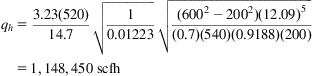
Example Problem 11.5 For the following data given for a horizontal pipeline, predict gas flow rate in ft3/hr through the pipeline. Solve the problem using Eq. (11.101) with the trial-and-error method for friction factor and the Weymouth equation without the Reynolds number–dependent friction factor:
Solution The average pressure is
With ![]() = 400 psia, T=540 °R and γg=0.70, Brill-Beggs-Z.xls gives
= 400 psia, T=540 °R and γg=0.70, Brill-Beggs-Z.xls gives
With ![]() 400 psia, T=540 °R and γg=0.70, Carr-Kobayashi-BurrowsViscosity.xls gives
400 psia, T=540 °R and γg=0.70, Carr-Kobayashi-BurrowsViscosity.xls gives
Relative roughness:
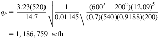
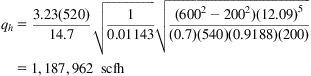

Problems similar to this one can be quickly solved with the spreadsheet program PipeCapacity.xls.
11.4.1.2.2 Weymouth equation for nonhorizontal flow
Gas transmission pipelines are often nonhorizontal. Account should be taken of substantial pipeline elevation changes. Considering gas flow from point 1 to point 2 in a nonhorizontal pipe, the first law of thermal dynamics gives
(11.104)
 (11.104)
Based on the pressure gradient due to the weight of gas column,
(11.105)
and real gas law, ![]() , Weymouth (1912) developed the following equation:
, Weymouth (1912) developed the following equation:
(11.106)
where
(11.107)
and Δz is equal to outlet elevation minus inlet elevation (note that Δz is positive when outlet is higher than inlet). A general and more rigorous form of the Weymouth equation with compensation for elevation is
(11.108)
where Le is the effective length of the pipeline. For a uniform slope, Le is defined as ![]() .
.
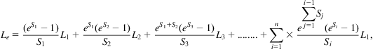
For a nonuniform slope (where elevation change cannot be simplified to a single section of constant gradient), an approach in steps to any number of sections, n, will yield
(11.109)
 (11.109)
where
(11.110)
11.4.1.2.3 Panhandle-A equation for horizontal flow
The Panhandle-A pipeline flow equation assumes the following Reynolds number–dependent friction factor:
(11.111)
The resultant pipeline flow equation is, thus,
(11.112)
where q is the gas flow rate in scfd measured at Tb and pb, and other terms are the same as in the Weymouth equation.
11.4.1.2.4 Panhandle-B equation for horizontal flow (modified Panhandle)
The Panhandle-B equation is the most widely used equation for long transmission and delivery lines. It assumes that fM varies as
(11.113)
and it takes the following resultant form:
(11.114)
11.4.1.2.5 Clinedinst equation for horizontal flow
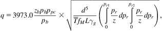
The Clinedinst equation rigorously considers the deviation of natural gas from ideal gas through integration. It takes the following form:
(11.115)
 (11.115)
ppc=pseudocritical pressure, psia
![]() =average flowing temperature, °R
=average flowing temperature, °R
zb=gas deviation factor at Tb and pb, normally accepted as 1.0.
Based on Eqs. (2.29), (2.30), and (2.51), Guo and Ghalambor (2005) generated curves of the integral function ![]() for various gas-specific gravity values.
for various gas-specific gravity values.
11.4.1.2.6 Pipeline efficiency
All pipeline flow equations were developed for perfectly clean lines filled with gas. In actual pipelines, water, condensates, sometimes crude oil accumulates in low spots in the line. There are often scales and even “junk” left in the line. The net result is that the flow rates calculated for the 100% efficient cases are often modified by multiplying them by an efficiency factor E. The efficiency factor expresses the actual flow capacity as a fraction of the theoretical flow rate. An efficiency factor ranging from 0.85 to 0.95 would represent a “clean” line. Table 11.1 presents typical values of efficiency factors.
11.4.2 Design of Pipelines
Pipeline design includes determination of material, diameter, wall thickness, insulation, and corrosion protection measure. For offshore pipelines, it also includes weight coating and trenching for stability control. Bai (2001) provides a detailed description on the analysis–based approach to designing offshore pipelines. Guo et al. (2005) presents a simplified approach to the pipeline design.
The diameter of pipeline should be determined based on flow capacity calculations presented in the previous section. This section focuses on the calculations to design wall thickness and insulation.
11.4.2.1 Wall thickness design
Wall thickness design for steel pipelines is governed by U.S. Code ASME/ANSI B32.8. Other codes such as Z187 (Canada), DnV (Norway), and IP6 (UK) have essentially the same requirements but should be checked by the readers.
Except for large-diameter pipes (>30 in.), material grade is usually taken as X-60 or X-65 (414 or 448 MPa) for high-pressure pipelines or in deepwater. Higher grades can be selected in special cases. Lower grades such as X-42, X-52, or X-56 can be selected in shallow water or for low-pressure, large-diameter pipelines to reduce material cost or in cases in which high ductility is required for improved impact resistance. Pipe types include:
Except in specific cases, only seamless or SAW pipes are to be used, with seamless being the preference for diameters of 12 in. or less. If ERW pipe is used, special inspection provisions such as full-body ultrasonic testing are required. Spiral weld pipe is very unusual for oil/gas pipelines and should be used only for low-pressure water or outfall lines.
11.4.2.1.1 Design procedure
Determination of pipeline wall thickness is based on the design internal pressure or the external hydrostatic pressure. Maximum longitudinal stresses and combined stresses are sometimes limited by applicable codes and must be checked for installation and operation. However, these criteria are not normally used for wall thickness determination. Increasing wall thickness can sometimes ensure hydrodynamic stability in lieu of other stabilization methods (such as weight coating). This is not normally economical, except in deepwater where the presence of concrete may interfere with the preferred installation method. We recommend the following procedure for designing pipeline wall thickness:
Step 1: Calculate the minimum wall thickness required for the design internal pressure.
Step 2: Calculate the minimum wall thickness required to withstand external pressure.
Step 3: Add wall thickness allowance for corrosion if applicable to the maximum of the above.
Step 4: Select next highest nominal wall thickness.
Step 5: Check selected wall thickness for hydrotest condition.
Step 6: Check for handling practice, that is, pipeline handling is difficult for D/t larger than 50; welding of wall thickness less than 0.3 in. (7.6 mm) requires special provisions.
Note that in certain cases, it may be desirable to order a nonstandard wall. This can be done for large orders.
Pipelines are sized on the basis of the maximum expected stresses in the pipeline under operating conditions. The stress calculation methods are different for thin-wall and thick-wall pipes. A thin-wall pipe is defined as a pipe with D/t greater than or equal to 20. Fig. 11.11 shows stresses in a thin-wall pipe. A pipe with D/t less than 20 is considered a thick-wall pipe. Fig. 11.12 illustrates stresses in a thick-wall pipe.


11.4.2.1.2 Design for internal pressure
Three pipeline codes typically used for design are ASME B31.4 (ASME, 1989), ASME B31.8 (ASME, 1990), and DnV (1981). ASME B31.4 is for all oil lines in North America. ASME B31.8 is for all gas lines and two-phase flow pipelines in North America. DnV (1981) is for oil, gas, and two-phase flow pipelines in North Sea. All these codes can be used in other areas when no other code is available.
The nominal pipeline wall thickness (tNOM) can be calculated as follows:
(11.116)
where Pd is the design internal pressure defined as the difference between the internal pressure (Pi) and external pressure (Pe), D is nominal outside diameter, ta is thickness allowance for corrosion, and is the specified minimum yield strength. Eq. (11.116) is valid for any consistent units.
Most codes allow credit for external pressure. This credit should be used whenever possible, although care should be exercised for oil export lines to account for head of fluid and for lines that traverse from deep to shallow water.
ASME B31.4 and DnV (1981) define Pi as the maximum allowable operating pressure (MAOP) under normal conditions, indicating that surge pressures up to 110% MAOP is acceptable. In some cases, Pi is defined as wellhead shut-in pressure (WSIP) for flowlines or specified by the operators.
In Eq. (11.116), the weld efficiency factor (Ew) is 1.0 for seamless, ERW, and DSAW pipes. The temperature de-rating factor (Ft) is equal to 1.0 for temperatures under 250°F. The usage factor (η) is defined in Tables 11.2 and 11.3 for oil and gas lines, respectively.
Table 11.2
Design and Hydrostatic Pressure Definitions and Usage Factors for Oil Lines
| Parameter | ASME B31.4, 1989 Edition | Dnv (Veritas, 1981) |
| Design internal pressure Pda | Pi–Pe [401.2.2] | Pi–Pe [4.2.2.2] |
| Usage factor η | 0.72 [402.3.1(a)] | 0.72 [4.2.2.1] |
| Hydrotest pressure Ph | 1.25 Pib [437.4.1(a)] | 1.25 Pd [8.8.4.3] |
aCredit can be taken for external pressure for gathering lines or flowlines when the MAOP (Pi) is applied at the wellhead or at the seabed. For export lines, when Pi is applied on a platform deck, the head fluid shall be added to Pi for the pipeline section on the seabed.
bIf hoop stress exceeds 90% of yield stress based on nominal wall thickness, special care should be taken to prevent overstrain of the pipe.
Table 11.3
Design and Hydrostatic Pressure Definitions and Usage Factors for Gas Lines
| Parameter | ASME B31.8, 1989 Edition, 1990 Addendum | DnV (Veritas, 1981) |
| Pda | Pi–Pe [A842.221] | Pi–Pe [4.2.2.2] |
| Usage factor η | 0.72 [A842.221] | 0.72 [4.2.2.1] |
| Hydrotest pressure Ph | 1.25 Pib [A847.2] | 1.25Pd [8.8.4.3] |
aCredit can be taken for external pressure for gathering lines or flowlines when the MAOP (Pi) is applied at wellhead or at the seabed. For export lines, when Pi is applied on a platform deck, the head of fluid shall be added to Pi for the pipeline section on the seabed (particularly for two-phase flow).
bASME B31.8 imposes Ph=1.4 Pi for offshore risers but allows onshore testing of prefabricated portions.
The under thickness due to manufacturing tolerance is taken into account in the design factor. There is no need to add any allowance for fabrication to the wall thickness calculated with Eq. (11.116).
11.4.2.1.3 Design for external pressure
Different practices can be found in the industry using different external pressure criteria. As a rule of thumb, or unless qualified thereafter, it is recommended to use propagation criterion for pipeline diameters under 16-in. and collapse criterion for pipeline diameters more than or equal to 16-in.
Propagation criterion
The propagation criterion is more conservative and should be used where optimization of the wall thickness is not required or for pipeline installation methods not compatible with the use of buckle arrestors such as reel and two methods. It is generally economical to design for propagation pressure for diameters less than 16-in. For greater diameters, the wall thickness penalty is too high. When a pipeline is designed based on the collapse criterion, buckle arrestors are recommended. The external pressure criterion should be based on nominal wall thickness, as the safety factors included below account for wall variations.
Although a large number of empirical relationships have been published, the recommended formula is the latest given by AGA.PRC (AGA, 1990):
(11.117)
which is valid for any consistent units. The nominal wall thickness should be determined such that Pp>1.3 Pe. The safety factor of 1.3 is recommended to account for uncertainty in the envelope of data points used to derive Eq. (11.117). It can be rewritten as
(11.118)
For the reel barge method, the preferred pipeline grade is below X-60. However, X-65 steel can be used if the ductility is kept high by selecting the proper steel chemistry and microalloying. For deepwater pipelines, D/t ratios of less than 30 are recommended. It has been noted that bending loads have no demonstrated influence on the propagation pressure.
Collapse criterion
The mode of collapse is a function of D/t ratio, pipeline imperfections, and load conditions. The theoretical background is not given in this book. An empirical general formulation that applies to all situations is provided. It corresponds to the transition mode of collapse under external pressure (Pe), axial tension (Ta), and bending strain (sb), as detailed elsewhere (Murphey and Langner, 1985; AGA, 1990).
The nominal wall thickness should be determined such that
(11.119)
where 1.3 is the recommended safety factor on collapse, BB is the bending strain of buckling failure due to pure bending, and g is an imperfection parameter defined below.
The safety factor on collapse is calculated for D/t ratios along with the loads (Pe, εb, Ta) and initial pipeline out-of roundness (δo). The equations are
(11.120)
(11.121)
 (11.121)
(11.122)
(11.123)
(11.124)
where gp is based on pipeline imperfections such as initial out-of roundness (δo), eccentricity (usually neglected), and residual stress (usually neglected). Hence,
(11.125)
 (11.125)
where
(11.126)
(11.127)
(11.128)
and
(11.129)
When a pipeline is designed using the collapse criterion, a good knowledge of the loading conditions is required (Ta and εb). An upper conservative limit is necessary and must often be estimated.
Under high bending loads, care should be taken in estimating εb using an appropriate moment-curvature relationship. A Ramberg Osgood relationship can be used as
(11.130)
where K*=K/Ky and M*=M/My with Ky=2Sy/ED is the yield curvature and My=2ISy/D is the yield moment. The coefficients A and B are calculated from the two data points on stress–strain curve generated during a tensile test.
11.4.2.1.4 Corrosion allowance
To account for corrosion when water is present in a fluid along with contaminants such as oxygen, hydrogen sulfide (H2S), and carbon dioxide (CO2), extra wall thickness is added. A review of standards, rules, and codes of practices (Hill and Warwick, 1986) shows that wall allowance is only one of several methods available to prevent corrosion, and it is often the least recommended.
For H2S and CO2 contaminants, corrosion is often localized (pitting) and the rate of corrosion allowance ineffective. Corrosion allowance is made to account for damage during fabrication, transportation, and storage. A value of ![]() in. may be appropriate. A thorough assessment of the internal corrosion mechanism and rate is necessary before any corrosion allowance is taken.
in. may be appropriate. A thorough assessment of the internal corrosion mechanism and rate is necessary before any corrosion allowance is taken.
11.4.2.1.5 Check for hydrotest condition
The minimum hydrotest pressure for oil and gas lines is given in Tables 11.2 and 11.3, respectively, and is equal to 1.25 times the design pressure for pipelines. Codes do not require that the pipeline be designed for hydrotest conditions but sometimes give a tensile hoop stress limit 90% SMYS, which is always satisfied if credit has not been taken for external pressure. For cases where the wall thickness is based on Pd=Pi–Pe, codes recommend not to overstrain the pipe. Some of the codes are ASME B31.4 (Clause 437.4.1), ASME B31.8 (no limit on hoop stress during hydrotest), and DnV (Clause 8.8.4.3).
For design purposes, condition σh≤σy should be confirmed, and increasing wall thickness or reducing test pressure should be considered in other cases. For offshore pipelines connected to riser sections requiring Ph=1.4Pi, it is recommended to consider testing the riser separately (for prefabricated sections) or to determine the hydrotest pressure based on the actual internal pressure experienced by the pipeline section. It is important to note that most pressure testing of subsea pipelines is done with water, but on occasion, nitrogen or air has been used. For low D/t ratios (<20), the actual hoop stress in a pipeline tested from the surface is overestimated when using the thin wall equations provided in this chapter. Credit for this effect is allowed by DnV Clause 4.2.2.2 but is not normally taken into account.
Example Problem 11.6 Calculate the required wall thickness for the pipeline in Example Problem 11.4 assuming a seamless still pipe of X-60 grade and onshore gas field (external pressure Pe=14.65 psia).
Solution The wall thickness can be designed based on the hoop stress generated by the internal pressure Pi=2590 psia. The design pressure is
The weld efficiency factor is Ew=1.0. The temperature de-rating factor Ft=1.0. Table 11.3 gives η=0.72. The yield stress is σy=60,000 psi. A corrosion allowance ![]() in. is considered. The nominal pipeline wall thickness can be calculated using Eq. (11.116) as
in. is considered. The nominal pipeline wall thickness can be calculated using Eq. (11.116) as
Considering that welding of wall thickness less than 0.3 in. requires special provisions, the minimum wall thickness is taken, 0.3 in.
11.4.2.2 Insulation design
Oil and gas field pipelines are insulated mainly to conserve heat. The need to keep the product fluids in the pipeline at a temperature higher than the ambient temperature could exist, for reasons including the following:
• Preventing formation of gas hydrates
• Preventing formation of wax or asphaltenes
In liquefied gas pipelines, such as liquefied natural gas, insulation is required to maintain the cold temperature of the gas to keep it in a liquid state.
Designing pipeline insulation requires thorough knowledge of insulation materials and heat transfer mechanisms across the insulation. Accurate predictions of heat loss and temperature profile in oil- and gas-production pipelines are essential to designing and evaluating pipeline operations.
11.4.2.2.1 Insulation materials
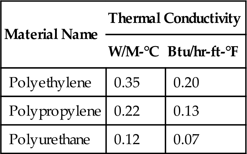
Polypropylene, polyethylene, and polyurethane are three base materials widely used in the petroleum industry for pipeline insulation. Their thermal conductivities are given in Table 11.4 (Carter et al., 2002). Depending on applications, these base materials are used in different forms, resulting in different overall conductivities. A three-layer polypropylene applied to pipe surface has a conductivity of 0.225 W/M-°C (0.13 btu/hr-ft-°F), while a four-layer polypropylene has a conductivity of 0.173 W/M-°C (0.10 btu/hr-ft-°F). Solid polypropylene has higher conductivity than polypropylene foam. Polymer syntactic polyurethane has a conductivity of 0.121 W/M-°C (0.07 btu/hr-ft-°F), while glass syntactic polyurethane has a conductivity of 0.156 W/M-°C (0.09 btu/hr-ft-°F). These materials have lower conductivities in dry conditions such as that in pipe-in-pipe (PIP) applications.
Table 11.4
Thermal Conductivities of Materials Used in Pipeline Insulation
| Material Name | Thermal Conductivity | |
| W/M-°C | Btu/hr-ft-°F | |
| Polyethylene | 0.35 | 0.20 |
| Polypropylene | 0.22 | 0.13 |
| Polyurethane | 0.12 | 0.07 |
Because of their low thermal conductivities, more and more polyurethane foams are used in deepwater pipeline applications. Physical properties of polyurethane foams include density, compressive strength, thermal conductivity, closed-cell content, leachable halides, flammability, tensile strength, tensile modulus, and water absorption. Typical values of these properties are available elsewhere (Guo et al., 2005).
In steady-state flow conditions in an insulated pipeline segment, the heat flow through the pipe wall is given by
(11.131)
where Qr is heat-transfer rate; U is overall heat-transfer coefficient (OHTC) at the reference radius; Ar is area of the pipeline at the reference radius; ΔT is the difference in temperature between the pipeline product and the ambient temperature outside.
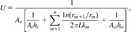
The OHTC, U, for a system is the sum of the thermal resistances and is given by (Holman, 1981):
(11.132)
 (11.132)
where hi is film coefficient of pipeline inner surface; ho is film coefficient of pipeline outer surface; Ai is area of pipeline inner surface; Ao is area of pipeline outer surface; rm is radius of layer m; and km is thermal conductivity of layer m.
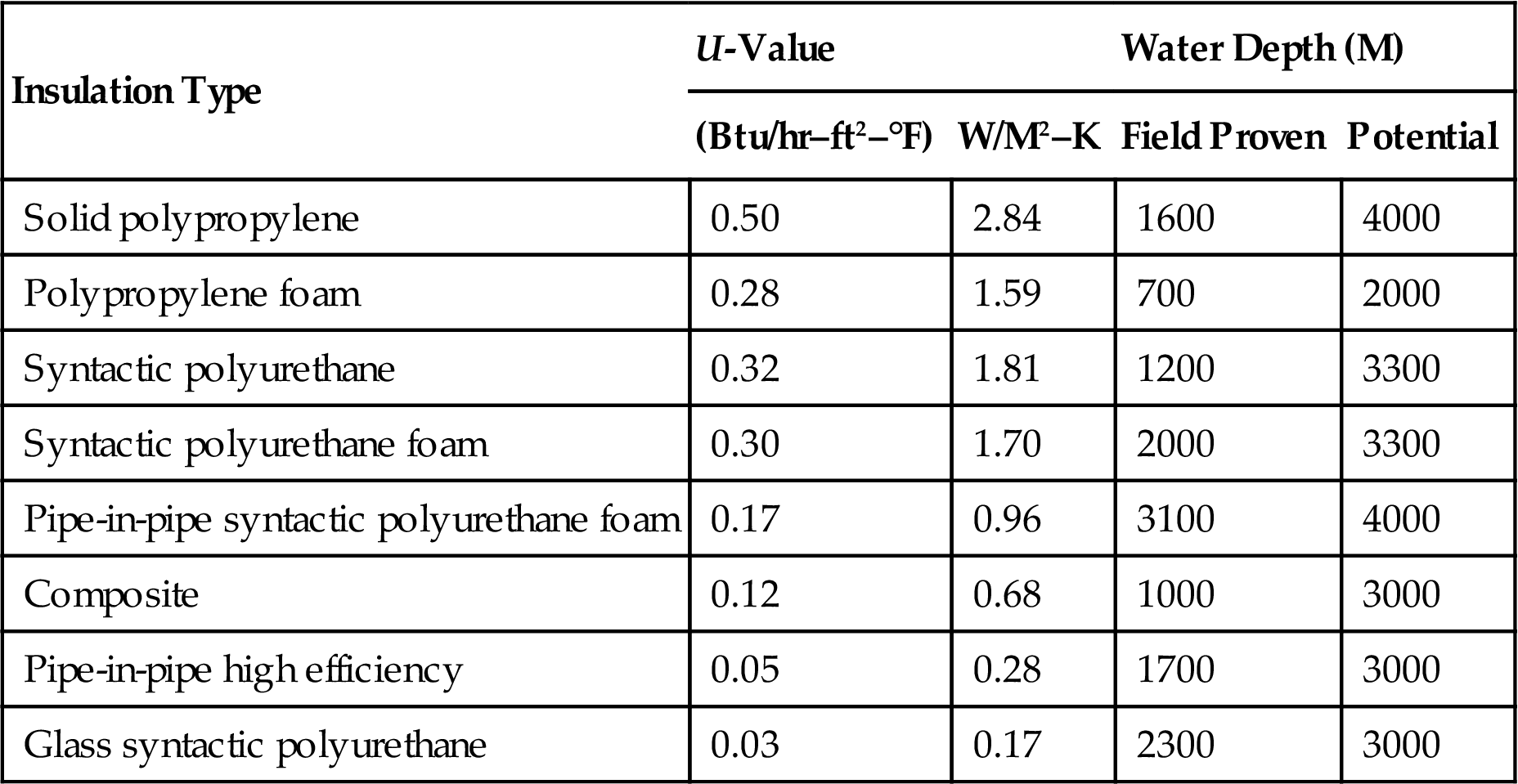
Similar equations exist for transient-heat flow, giving an instantaneous rate for heat flow. Typically required insulation performance, in terms of OHTC (U value) of steel pipelines in water, is summarized in Table 11.5.
Table 11.5
Typical Performance of Insulated Pipelines
| Insulation Type | U-Value | Water Depth (M) | ||
| (Btu/hr–ft2–°F) | W/M2–K | Field Proven | Potential | |
| Solid polypropylene | 0.50 | 2.84 | 1600 | 4000 |
| Polypropylene foam | 0.28 | 1.59 | 700 | 2000 |
| Syntactic polyurethane | 0.32 | 1.81 | 1200 | 3300 |
| Syntactic polyurethane foam | 0.30 | 1.70 | 2000 | 3300 |
| Pipe-in-pipe syntactic polyurethane foam | 0.17 | 0.96 | 3100 | 4000 |
| Composite | 0.12 | 0.68 | 1000 | 3000 |
| Pipe-in-pipe high efficiency | 0.05 | 0.28 | 1700 | 3000 |
| Glass syntactic polyurethane | 0.03 | 0.17 | 2300 | 3000 |
Pipeline insulation comes in two main types: dry insulation and wet insulation. The dry insulations require an outer barrier to prevent water ingress (PIP). The most common types of this include the following:
Under certain conditions, PIP systems may be considered over conventional single-pipe systems. PIP insulation may be required to produce fluids from high-pressure/high-temperature (>150°C) reservoirs in deepwater (Carmichael et al., 1999). The annulus between pipes can be filled with different types of insulation materials such as foam, granular particles, gel, and inert gas or vacuum.
A pipeline-bundled system—a special configuration of PIP insulation—can be used to group individual flowlines together to form a bundle (McKelvie, 2000); heat-up lines can be included in the bundle, if necessary. The complete bundle may be transported to site and installed with a considerable cost savings relative to other methods. The extra steel required for the carrier pipe and spacers can sometimes be justified (Bai, 2001).
Wet-pipeline insulations are those materials that do not need an exterior steel barrier to prevent water ingress, or the water ingress is negligible and does not degrade the insulation properties. The most common types of this are as follows:
The main materials that have been used for deepwater insulations have been polyurethane and polypropylene based. Syntactic versions use plastic or glass matrix to improve insulation with greater depth capabilities. Insulation coatings with combinations of the two materials have also been used. Guo et al. (2005) gives the properties of these wet insulations. Because the insulation is buoyant, this effect must be compensated by the steel pipe weight to obtain lateral stability of the deepwater pipeline on the seabed.
11.4.2.2.2 Heat transfer models
Heat transfer across the insulation of pipelines presents a unique problem affecting flow efficiency. Although sophisticated computer packages are available for predicting fluid temperatures, their accuracies suffer from numerical treatments because long pipe segments have to be used to save computing time. This is especially true for transient fluid-flow analyses in which a very large number of numerical iterations are performed.
Ramey (1962) was among the first investigators who studied radial-heat transfer across a well casing with no insulation. He derived a mathematical heat-transfer model for an outer medium that is infinitely large. Miller (1980) analyzed heat transfer around a geothermal wellbore without insulation. Winterfeld (1989) and Almehaideb et al. (1989) considered temperature effect on pressure-transient analyses in well testing. Stone et al. (1989) developed a numerical simulator to couple fluid flow and heat flow in a wellbore and reservoir. More advanced studies on the wellbore heat-transfer problem were conducted by Hasan and Kabir (1994, 2002), Hasan et al. (1997, 1998), and Kabir et al. (1996). Although multilayers of materials have been considered in these studies, the external temperature gradient in the longitudinal direction has not been systematically taken into account. Traditionally, if the outer temperature changes with length, the pipe must be divided into segments, with assumed constant outer temperature in each segment, and numerical algorithms are required for heat-transfer computation. The accuracy of the computation depends on the number of segments used. Fine segments can be employed to ensure accuracy with computing time sacrificed.
Guo et al. (2006) presented three analytical heat-transfer solutions. They are the transient-flow solution for startup mode, steady-flow solution for normal operation mode, and transient-flow solution for flow rate change mode (shutting down is a special mode in which the flow rate changes to zero).
Temperature and heat transfer for steady fluid flow
The internal temperature profile under steady fluid-flow conditions is expressed as
(11.133)
where the constant groups are defined as
(11.134)
(11.135)
(11.136)
and
(11.137)
where T is temperature inside the pipe, L is longitudinal distance from the fluid entry point, R is inner radius of insulation layer, k is the thermal conductivity of the insulation material, v is the average flow velocity of fluid in the pipe, ρ is fluid density, Cp is heat capacity of fluid at constant pressure, s is thickness of the insulation layer, A is the inner cross-sectional area of pipe, G is principal thermal-gradient outside the insulation, θ is the angle between the principal thermal gradient and pipe orientation, T0 is temperature of outer medium at the fluid entry location, and Ts is temperature of fluid at the fluid entry point.
The rate of heat transfer across the insulation layer over the whole length of the pipeline is expressed as
(11.138)
where q is the rate of heat transfer (heat loss).
Transient temperature during startup
The internal temperature profile after starting up a fluid flow is expressed as follows:
(11.139)
where the function f is given by
(11.140)
and t is time.
Transient temperature during flow rate change
Suppose that after increasing or decreasing the flow rate, the fluid has a new velocity v′ in the pipe. The internal temperature profile is expressed as follows:
(11.141)
where
(11.142)
(11.143)
(11.144)
and the function f is given by
(11.145)
Example Problem 11.7 A design case is shown in this example. Design base for a pipeline insulation is presented in Table 11.6. The design criterion is to ensure that the temperature at any point in the pipeline will not drop to less than 25°C, as required by flow assurance. Insulation materials considered for the project were polyethylene, polypropylene, and polyurethane.
Table 11.6
Base Data for Pipeline Insulation Design
| Length of pipeline: | 8047 | M |
| Outer diameter of pipe: | 0.2032 | M |
| Wall thickness: | 0.00635 | M |
| Fluid density: | 881 | kg/M3 |
| Fluid specific heat: | 2012 | J/kg-°C |
| Average external temperature: | 10 | °C |
| Fluid temperature at entry point: | 28 | °C |
| Fluid flow rate: | 7950 | M3/day |
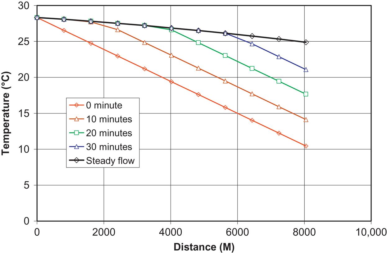
Solution A polyethylene layer of 0.0254 M (1 in.) was first considered as the insulation. Fig. 11.13 shows the temperature profiles calculated using Eqs. (11.133) and (11.139). It indicates that at approximately 40 minutes after startup, the transient-temperature profile in the pipeline will approach the steady-flow temperature profile. The temperature at the end of the pipeline will be slightly lower than 20°C under normal operating conditions. Obviously, this insulation option does not meet design criterion of 25°C in the pipeline.
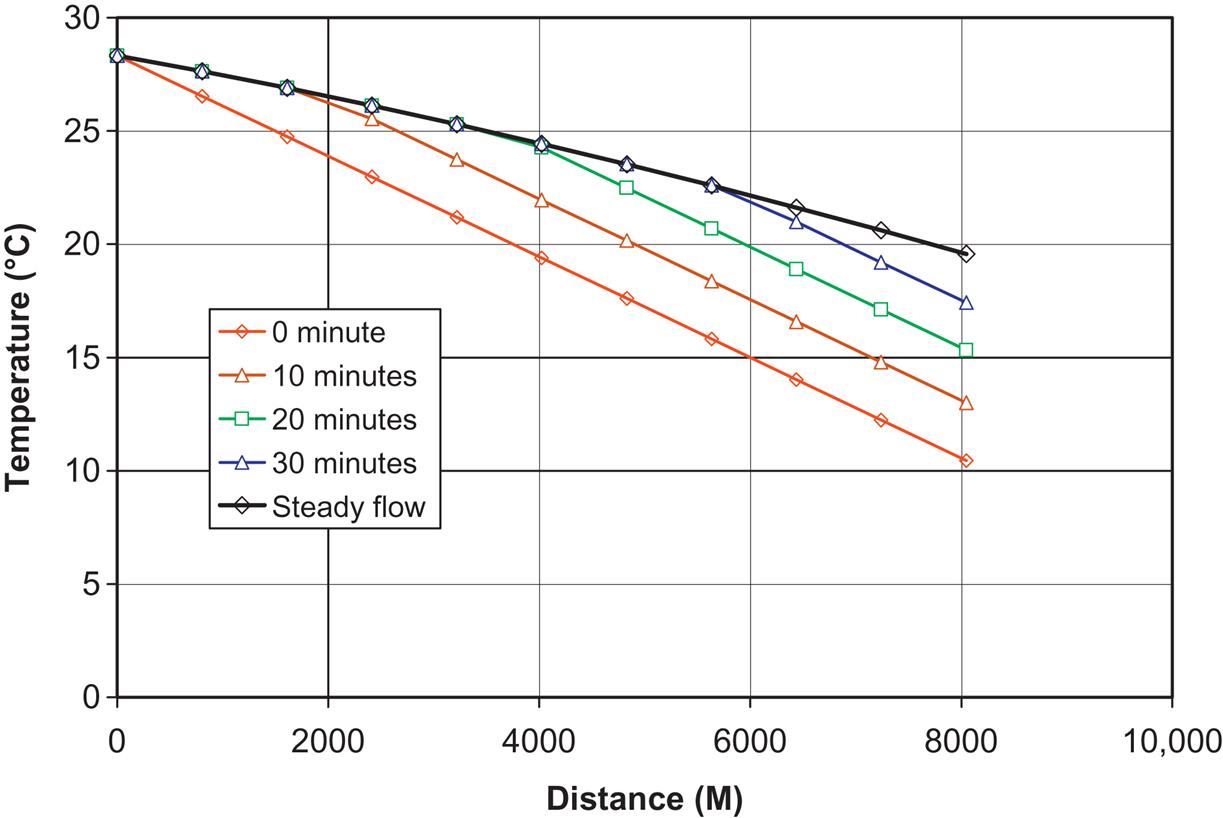
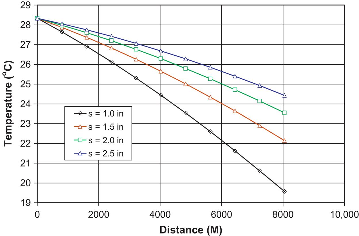
Fig. 11.14 presents the steady-flow temperature profiles calculated using Eq. (11.133) with polyethylene layers of four thicknesses. It shows that even a polyethylene layer 0.0635-M (2.5-in.) thick will still not give a pipeline temperature higher than 25°C; therefore, polyethylene should not be considered in this project.
A polypropylene layer of 0.0254 M (1 in.) was then considered as the insulation. Fig. 11.15 illustrates the temperature profiles calculated using Eq. (11.133) and (11.139). It again indicates that at approximately 40 minutes after startup, the transient-temperature profile in the pipe will approach the steady-flow temperature profile. The temperature at the end of the pipeline will be approximately 22.5°C under normal operating conditions. Obviously, this insulation option, again, does not meet design criterion of 25°C in the pipeline.

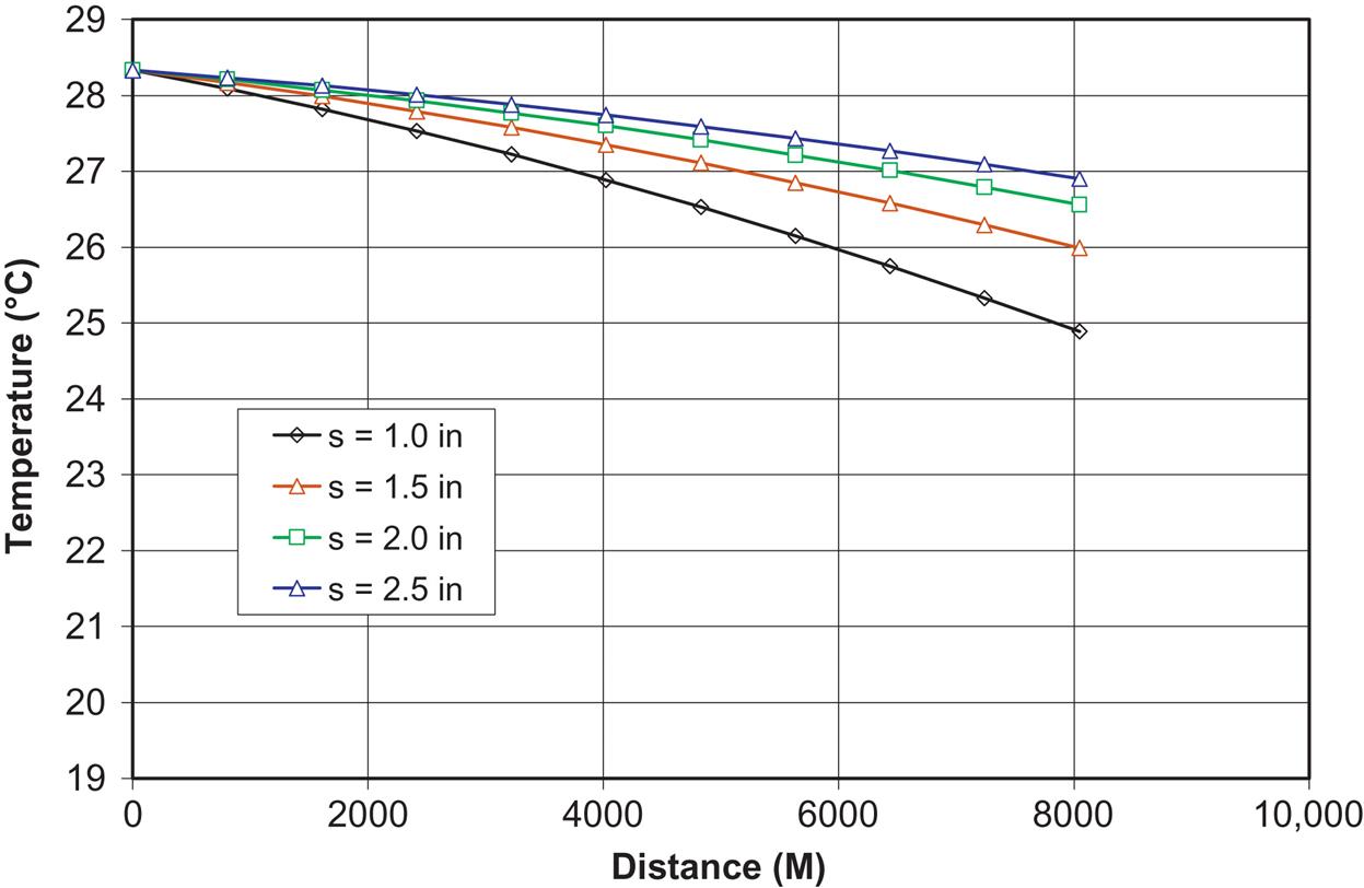
Fig. 11.16 demonstrates the steady-flow temperature profiles calculated using Eq. (11.133) with polypropylene layers of four thicknesses. It shows that a polypropylene layer of 0.0508 M (2.0 in.) or thicker will give a pipeline temperature of higher than 25°C.

A polyurethane layer of 0.0254 M (1 in.) was also considered as the insulation. Fig. 11.17 shows the temperature profiles calculated using Eqs. (11.133) and (11.139). It indicates that the temperature at the end of pipeline will drop to slightly lower than 25°C under normal operating conditions. Fig. 11.18 presents the steady-flow temperature profiles calculated using Eq. (11.133) with polyurethane layers of four thicknesses. It shows that a polyurethane layer of 0.0381 M (1.5 in.) is required to keep pipeline temperatures higher than 25°C under normal operating conditions.
Therefore, either a polypropylene layer of 0.0508 M (2.0 in.) or a polyurethane layer of 0.0381 M (1.5 in.) should be chosen for insulation of the pipeline. Cost analyses can justify one of the options, which is beyond the scope of this example.
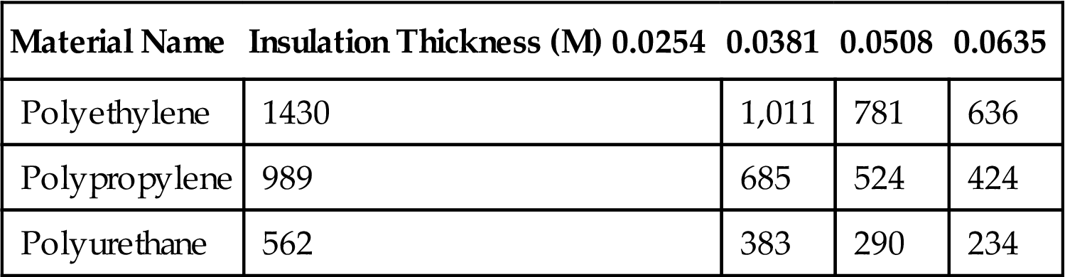
The total heat losses for all the steady-flow cases were calculated with Eq. (11.138). The results are summarized in Table 11.7. These data may be used for sizing heaters for the pipeline if heating of the product fluid is necessary.
11.5 Summary
This chapter described oil and gas transportation systems. The procedure for selection of pumps and gas compressors were presented and demonstrated. Theory and applications of pipeline design were illustrated.
Problems
11.1 A pipeline transporting 10,000 bbl/day of oil requires a pump with a minimum output pressure of 500 psi. The available suction pressure is 300 psi. Select a triplex pump for this operation.
11.2 A pipeline transporting 8000 bbl/day of oil requires a pump with a minimum output pressure of 400 psi. The available suction pressure is 300 psi. Select a duplex pump for this operation.
11.3 For a reciprocating compressor, calculate the theoretical and brake horsepower required to compress 30 MMcfd of a 0.65 specific gravity natural gas from 100 psia and 70°F to 2000 psia. If intercoolers and end-coolers cool the gas to 90°F, what is the heat load on the coolers? Assuming the overall efficiency is 0.80.
11.4 For a centrifugal compressor, use the following data to calculate required input horsepower and polytropic head:
| Gas-specific gravity: | 0.70 |
| Gas-specific heat ratio: | 1.30 |
| Gas flow rate: | 50 MMscfd at 14.7 psia and 60°F |
| Inlet pressure: | 200 psia Inlet temperature: 70°F |
| Discharge pressure: | 500 psia |
| Polytropic efficiency: | Ep=061+003 log (q1) |
11.5 For the data given in Problem 11.4, calculate the required brake horsepower if a reciprocating compressor is used.
11.6 A 40-API gravity, 3-cp oil is transported through an 8-in. (I.D.) pipeline with a downhill angle of 5° across a distance of 10 miles at a flow rate of 5000 bbl/day. Estimate the minimum required pump pressure to deliver oil at 100 psi pressure at the outlet. Assume e=0.0006 in.
11.7 For the following data given for a horizontal pipeline, predict gas flow rate in cubic feet per hour through the pipeline. Solve the problem using Eq. (11.101) with the trial-and-error method for friction factor and the Weymouth equation without the Reynolds number–dependent friction factor:
d=6 in.
L=100 mi
e=0.0006 in.
T=70°F
γg=0.70
Tb=520°R
pb=14.65 psia
p1=800 psia
p2=200 psia
11.9 Assuming a 10° uphill angle, solve Problem using the Weymouth equation.
11.10 Calculate the required wall thickness for a pipeline using the following data:
Water depth 2000 ft offshore oil field
Water temperature 45°F
12.09 in. pipe inner diameter
Seamless still pipe of X-65 grade
Maximum pipeline pressure 3000 psia
11.11 Design insulation for a pipeline with the following given data:
| Length of pipeline: | 7000 M |
| Outer diameter of pipe: | 0.254 M |
| Wall thickness: | 0.0127 M |
| Fluid density: | 800 kg/M3 |
| Fluid specific heat: | 2000 J/kg-°C |
| Average external temperature: | 15°C |
| Fluid temperature at entry point: | 30°C |
| Fluid flow rate: | 5000 M3/day |