11.2.1 Triplex Pumps

The work per stroke for a single piston is expressed as

${\overline{W}}_1=P\left(\frac{\pi D^2}{4}\right)L(\mathrm{ft}-\text{lbs}).$

The work per one rotation of crank is

${\overline{W}}_2=P\left(\frac{\pi D^2}{4}\right)L(1)\left(\frac{\mathrm{ft}-\mathrm{l}\mathrm{bs}}{\mathrm{rotation}}\right).$

where

Thus, for a triplex pump, the theoretical power is

$\mathrm{Power}=3P\left(\frac{\pi D^2}{4}\right)LN\left(\frac{\mathrm{ft}-\mathrm{lb}}{\min }\right),$ (11.1)

(11.1)

where N is pumping speed in strokes per minute. The theoretical horsepower is

$H{P}_{th}=\frac{3P\left(\frac{\pi D^2}{4}\right)}{550(60)}LN(\mathrm{hp})$ (11.2)

(11.2)

or

$H{P}_{th}=\frac{3P\left(\frac{\pi D^2}{4}\right)}{33,000}LN(\mathrm{hp}).$ (11.3)

(11.3)

The input horsepower needed from the prime mover is

$H{P}_i=\frac{3P\left(\frac{\pi D^2}{4}\right)}{33,000e_m}LN(\mathrm{hp}),$ (11.4)

(11.4)

where e_m is the mechanical efficiency of the mechanical system transferring power from the prime mover to the fluid in the pump. Usually e_m is taken to be about 0.85.

The theoretical volume output from a triplex pump per revolution is

$Q_{th}=3\left(\frac{\pi D^2}{4}\right)\frac{LN}{60}({\mathrm{ft}}^3/\text{sec}).$ (11.5)

(11.5)

The theoretical output in bbl/day is thus

$q_{th}=604LN{D}^2\left(\frac{\mathrm{bbl}}{\mathrm{day}}\right).$ (11.6)

(11.6)

If we use inches (i.e., d [in.] and l [in.]), for D and L, then

$q_{th}=0.35lN{d}^2\left(\frac{\mathrm{bbl}}{\mathrm{day}}\right).$ (11.7)

(11.7)

The real output of the pump is dependent on how efficiently the pump can fill the chambers of the pistons. Using the volumetric efficiency e_v in Eq. 11.7 gives

$q_r=0.35e_{v}lN{d}^2\left(\frac{\mathrm{bbl}}{\mathrm{day}}\right)$ (11.8)

(11.8)

or

$q_r=0.01e_v{d}^{2}lN(\mathrm{gal}/\min ),$ (11.9)

(11.9)

where e_v is usually taken to be 0.88–0.98.

As the above volumetric equation can be written in d and l, then the horsepower equation can be written in d, l, and p (psi). Thus,

$H{P}_i=\frac{3p\left(\frac{\pi d^2}{4}\right)\frac{1}{12}N}{33,000e_m}$ (11.10)

(11.10)

reduces to

$H{P}_i=\frac{p{d}^{2}lN}{168,067e_m}.$ (11.11)

(11.11)

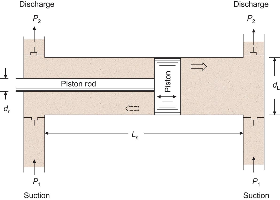
11.2.2 Duplex Pumps

The work per stroke cycle is expressed as

$W_1=P\left(\frac{\pi D_1^2}{4}\right)L+P\left[\frac{\pi D_1^2}{4}-\frac{\pi D_2^2}{4}\right]L(\text{ft}-\text{lbs}).$ (11.12)

(11.12)

The work per one rotation of crank is

$W_2=\left\{P\left(\frac{\pi D_1^2}{4}\right)L+P\left[\frac{\pi D_1^2}{4}-\frac{\pi D_2^2}{4}\right]L\right\}(1)\left(\frac{\mathrm{ft}-\mathrm{lbs}}{\mathrm{rotation}}\right).$ (11.13)

(11.13)

Thus, for a duplex pump, the theoretical power is

$\mathit{Power}=2\times \left\{P\left(\frac{\pi D_1^2}{4}\right)L+P\left[\frac{\pi D_1^2}{4}-\frac{\pi D_2^2}{4}\right]L\right\}N\left(\frac{\mathrm{ft}-\mathrm{lbs}}{\min }\right).$ (11.14)

(11.14)

The theoretical horsepower is

$H{P}_{th}=\frac{2\left\{P\left(\frac{\pi D_1^2}{4}\right)L+P\left[\frac{\pi D_1^2}{4}-\frac{\pi D_2^2}{4}\right]L\right\}N}{550(60)}(\mathrm{hp})$

or

$H{P}_{th}=\frac{2\left\{P\left({\displaystyle \frac{\pi }{4}}{D}_1^2\right)L+P\left[\frac{\pi D_1^2}{4}-\frac{\pi D_2^2}{4}\right]L\right\}N}{33,000}.$ (11.15)

(11.15)

The input horsepower needed from the prime mover is

$Q_{th}=\frac{2\left\{P\left(\frac{\pi }{4}{D}_1^2\right)L+P\left[\frac{\pi D_1^2}{4}-\frac{\pi D_2^2}{4}\right]L\right\}N}{33,000e_m}(\mathrm{hp}).$ (11.16)

(11.16)

The theoretical volume output from the double-acting duplex pump per revolution is

$Q_{th}=2\left\{\frac{\pi D_1^2}{4}L+\left[\frac{\pi D_1^2}{4}-\frac{\pi D_2^2}{4}\right]L\right\}\frac{N}{60}({\mathrm{ft}}^3/\text{sec}).$ (11.17)

(11.17)

The theoretical output in gals/min is thus

$\begin{array}{ll}{q}_{th}\hfill & =2\left\{\frac{\pi D_1^2}{4}L+\left[\frac{\pi D_1^2}{4}-\frac{\pi D_2^2}{4}\right]L\right\}\times \frac{N}{0.1337}(\mathrm{gal}/\min ).\hfill \end{array}$ (11.18)

(11.18)

If we use inches (i.e., d [in.] and l [in.]), for D and L, then

$q_{th}=2\left\{\frac{\pi d_1^2}{4}l+\left[\frac{\pi d_1^2}{4}-\frac{\pi d_2^2}{4}\right]l\right\}\frac{N}{231}(\mathrm{gal}/\min ).$ (11.19)

(11.19)

The real output of the pump is

$q_r=2\left\{\frac{\pi d_1^2}{4}l+\left[\frac{\pi d_1^2}{4}-\frac{\pi d_2^2}{4}\right]l\right\}\frac{N}{231}{e}_v(\mathrm{gal}/\min )$

or

$q_r=0.0068(2d_1^2-d_2^2)lN{e}_V(\mathrm{gal}/\min ),$ (11.20)

(11.20)

that is,

$q_r=0.233(2d_1^2-d_2^2)lN{e}_{\mathrm{v}}(\text{bbl}/\text{day}).$ (11.21)

(11.21)

As in the volumetric output, the horsepower equation can also be reduced to a form with p, d₁, d₂, and l

$H{P}_i=\frac{p\left(2d_1^2-d_2^2\right)lN}{252,101e_m}.$ (11.22)

(11.22)

Returning to Eq. (11.16) for the duplex double-action pump, let us derive a simplified pump equation. Rewriting Eq. (11.16), we have

$H{P}_i=\frac{2\left\{P\left(\frac{\pi }{4}{D}_1^2\right)L+P\left[\frac{\pi D_1^2}{4}-\frac{\pi D_2^2}{4}\right]L\right\}N}{33,000e_m}.$ (11.23)

(11.23)

The flow rate is

$Q_{th}=2\left\{\frac{\pi D_1^2}{4}L+\left[\frac{\pi D_1^2}{4}-\frac{\pi D_2^2}{4}\right]L\right\}N({\mathrm{ft}}^3/\min ),$ (11.24)

(11.24)

so

$H{P}_i=\frac{P{Q}_{th}}{33,000e_m}$ (11.25)

(11.25)

The usual form of this equation is in p (psi) and q (gal/min):

$H{P}_i=\frac{\left[p{(12)}^2\right]\left[q(0.1337)\right]}{33,000e_m},$ (11.26)

(11.26)

that is,

$H{P}_i=\frac{pq}{1714e_m}.$ (11.27)

(11.27)

The other form of this equation is in p (psi) and q_o (bbl/day) for oil transportation:

$H{P}_i=\frac{p{q}_o}{58,766e_m}.$ (11.28)

(11.28)

Eqs. (11.27) and (11.28) are valid for any type of pump.

Example Problem 11.1 A pipeline transporting 5000 bbl/day of oil requires a pump with a minimum output pressure of 1000 psi. The available suction pressure is 300 psi. Select a triplex pump for this operation.

Solution Assuming a mechanical efficient of 0.85, the horsepower requirement is

$H{P}_i=\frac{p{q}_o}{58,766e_m}=\frac{(1000)(5000)}{58,766(0.85)}=100\mathrm{hp}.$

According to a product sheet of the Oilwell Plunger Pumps, the Model 336-ST Triplex with forged steel fluid end has a rated brake horsepower of 160 hp at 320 rpm. The maximum working pressure is 3180 psi with the minimum plunger (piston) size of 1¾ in. It requires a suction pressure of 275 psi. With 3-in. plungers, the pump displacement is 0.5508 gal/rpm, and it can deliver liquid flow rates in the range of 1889 bbl/day (55.08 gpm) at 100 rpm to 6046 bbl/day (176.26 gpm) at 320 rpm, allowing a maximum pressure of 1420 psi. This pump can be selected for the operation. The required operating rpm is

$\mathrm{RPM}=\frac{(5000)(42)}{(24)(60)(0.5508)}=265\mathrm{rpm}.$

11.3.1 Types of Compressors

The compressors used in today's natural gas production industry fall into two distinct types: reciprocating and rotary compressors. Reciprocating compressors are most commonly used in the natural gas industry. They are built for practically all pressures and volumetric capacities. As shown in Fig. 11.3, reciprocating compressors have more moving parts and, therefore, lower mechanical efficiencies than rotary compressors. Each cylinder assembly of a reciprocation compressor consists of a piston, cylinder, cylinder heads, suction and discharge valves, and other parts necessary to convert rotary motion to reciprocation motion. A reciprocating compressor is designed for a certain range of compression ratios through the selection of proper piston displacement and clearance volume within the cylinder. This clearance volume can be either fixed or variable, depending on the extent of the operation range and the percent of load variation desired. A typical reciprocating compressor can deliver a volumetric gas flow rate of up to 30,000 cubic feet per minute (cfm) at a discharge pressure of up to 10,000 psig.

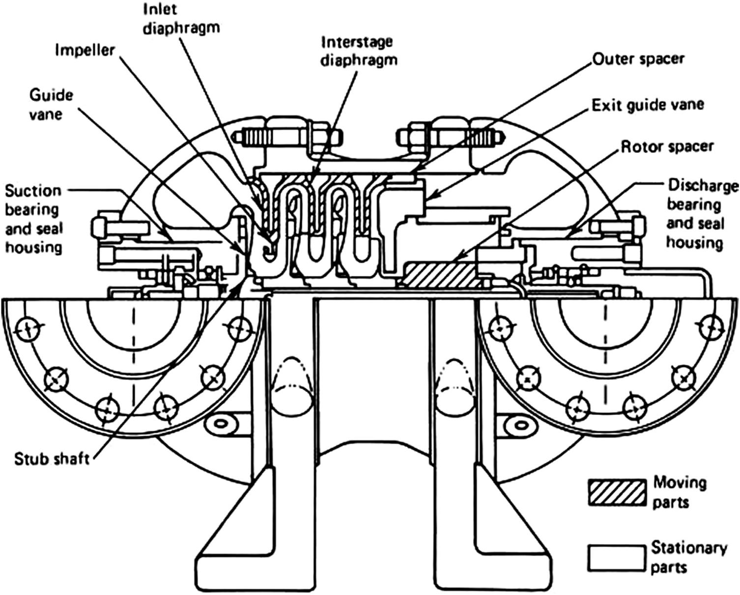
Rotary compressors are divided into two classes: the centrifugal compressor and the rotary blower. A centrifugal compressor (Fig. 11.4) consists of a housing with flow passages, a rotating shaft on which the impeller is mounted, bearings, and seals to prevent gas from escaping along the shaft. Centrifugal compressors have few moving parts because only the impeller and shaft rotate. Thus, its efficiency is high and lubrication oil consumption and maintenance costs are low. Cooling water is normally unnecessary because of lower compression ratio and lower friction loss. Compression rates of centrifugal compressors are lower because of the absence of positive displacement. Centrifugal compressors compress gas using centrifugal force. In this type of compressor, work is done on the gas by an impeller. Gas is then discharged at a high velocity into a diffuser where the velocity is reduced and its kinetic energy is converted to static pressure. Unlike reciprocating compressors, all this is done without confinement and physical squeezing. Centrifugal compressors with relatively unrestricted passages and continuous flow are inherently high-capacity, low-pressure ratio machines that adapt easily to series arrangements within a station. In this way, each compressor is required to develop only part of the station compression ratio. Typically, the volume is more than 100,000 cfm and discharge pressure is up to 100 psig.

A rotary blower is built of a casing in which one or more impellers rotate in opposite directions. Rotary blowers are primarily used in distribution systems where the pressure differential between suction and discharge is less than 15 psi. They are also used for refrigeration and closed regeneration of adsorption plants. The rotary blower has several advantages: large quantities of low-pressure gas can be handled at comparatively low horsepower, it has small initial cost and low maintenance cost, it is simple to install and easy to operate and attend, it requires minimum floor space for the quantity of gas removed, and it has almost pulsation-less flow. As its disadvantages, it cannot withstand high pressures, it has noisy operation because of gear noise and clattering impellers, it improperly seals the clearance between the impellers and the casing, and it overheats if operated above safe pressures. Typically, rotary blowers deliver a volumetric gas flow rate of up to 17,000 cfm and have a maximum intake pressure of 10 psig and a differential pressure of 10 psi.

When selecting a compressor, the pressure–volume characteristics and the type of driver must be considered. Small rotary compressors (vane or impeller type) are generally driven by electric motors. Large-volume positive compressors operate at lower speeds and are usually driven by steam or gas engines. They may be driven through reduction gearing by steam turbines or an electric motor. Reciprocation compressors driven by steam turbines or electric motors are most widely used in the natural gas industry as the conventional high-speed compression machine. Selection of compressors requires considerations of volumetric gas deliverability, pressure, compression ratio, and horsepower.

The following are important characteristics of the two types of compressors:

11.3.2 Reciprocating Compressors

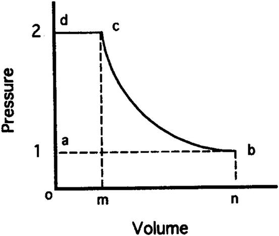
Fig. 11.5 shows a diagram volume relation during gas compression. The shaft work put into the gas is expressed as

$W_s=\frac{V_2^2}{2g}-\frac{V_1^2}{2g}+\left(P_2{v}_2-\underset{1}{\overset{2}{\int }}Pdv-P_1{v}_1\right),$ (11.29)

(11.29)

where

Note that the mechanical kinetic energy term $\frac{V^2}{2g}$ is in ft$\left(\frac{\mathrm{lb}}{\mathrm{lb}}\right)$ to get ft-lbs per lb.

Rewriting Eq. (11.29), we can get

$W_s+\frac{V_1^2}{2g}-\frac{V_2^2}{2g}+P_1{v}_1-P_2{v}_2=-\underset{1}{\overset{2}{\int }}Pdv.$ (11.30)

(11.30)

An isentropic process is usually assumed for reciprocating compression, that is, $P_1{v}_1^k=P_2{v}_2^k=P{v}^k=\mathrm{constant},$ where $k=\frac{c_p}{c_v}$. Because $P=\frac{P_1{v}_1^k}{V^k},$ the right-hand side of Eq. (11.30) is formulated as

$\begin{array}{ll}-\underset{1}{\overset{2}{\int }}pdv\hfill & =-\underset{1}{\overset{2}{\int }}\frac{P_1{v}_1^k}{v^k}dv=-P_1{v}_1^k\underset{1}{\overset{2}{\int }}\frac{dv}{v^k}\hfill \\ \hfill & =-P_1{v}_1^k{\left[\frac{v^{1-k}}{1-k}\right]}_1^2=-\frac{P_1{v}_1^k}{1-k}\left[v_2^{1-k}-v_1^{1-k}\right]\hfill \\ \hfill & =\frac{P_1{v}_1^k}{1-k}\left(\frac{v_1^{1-k}}{v_1^{1-k}}\right)\left[v_2^{1-k}-v_1^{1-k}\right]\hfill \\ \hfill & =\frac{P_1{v}_1}{1-k}\left[\frac{v_2^{1-k}}{v_1^{1-k}}-1\right]\hfill \\ \hfill & =\frac{P_1{v}_1}{1-k}\left[{\left({\displaystyle \frac{v_1}{v_2}}\right)}^{k-1}-1\right].\hfill \end{array}$ (11.31)

(11.31)

Using the ideal gas law

$\frac{P}{\gamma }=RT,$ (11.32)

(11.32)

where γ (lb/ft³) is the specific weight of the gas and T (°R) is the temperature and R=53.36 (lb-ft/lb-°R) is the gas constant, and $v=\frac{1}{\gamma },$ we can write Eq. (11.32) as

$Pv=RT$ (11.33)

(11.33)

or

$P_1{v}_1=R{T}_1.$ (11.34)

(11.34)

Using $P_1{v}_1^k=P_2{v}_2^k=P{v}^k=$ constant, which gives

${\left(\frac{v_1}{v_2}\right)}^k=\frac{P_2}{P_1}$

or

$\frac{v_1}{v_2}={\left(\frac{P_2}{P_1}\right)}^{\frac{1}{k}}.$ (11.35)

(11.35)

Substituting Eqs. (11.35) and (11.34) into Eq. (11.31) gives

$-\underset{1}{\overset{2}{\int }}Pdv=\frac{R{T}_1}{k-1}\left[{\left(\frac{P_2}{P_1}\right)}^{\frac{k-1}{k}}-1\right].$ (11.36)

(11.36)

We multiply Eq. (11.33) by v^k−1, which gives

$\begin{array}{l}Pv(v^{k-1})=RT(v^{k-1})\hfill \\ P{v}^k=RT{v}^{k-1}=C_1\hfill \\ \frac{P{v}^k}{R}=T{v}^{k-1}=\frac{C_1}{R}={C\prime }_1\hfill \end{array}$

Thus,

$T{v}^{k-1}={C\prime }_1.$ (11.37)

(11.37)

Also we can rise $P{v}^k$ = constant to the $\left(\frac{k-1}{k}\right)$ power. This is

$\begin{array}{l}{(P{v}^k)}^{\frac{k-1}{k}}={{C\prime }_1}^{\frac{k-1}{k}}\hfill \\ P^{\frac{k-1}{k}}{v}^{k-1}={{C\prime }_1}^{\frac{k-1}{k}}\hfill \end{array}$

or

$v^{k-1}=\frac{C_1^{\frac{\text{'}k-1}{k}}}{P^{\frac{k-1}{k}}}=\frac{C_1^n}{P^{\frac{k-1}{k}}}.$ (11.38)

(11.38)

Substituting Eq. (11.38) into (11.37) gives

$T\frac{{C\prime }_1}{P^{\frac{k-1}{k}}}={C\prime }_1$

or

$\frac{T}{P^{\frac{k-1}{k}}}=\frac{{C\prime }_1}{{C\prime }_1}={C\prime \prime }_1=\mathrm{constant}.$ (11.39)

(11.39)

Thus, Eq. (11.39) can be written as

$\frac{T_1}{P_1^{\frac{k-1}{k}}}=\frac{T_2}{P_2^{\frac{k-1}{k}}}.$ (11.40)

(11.40)

Thus, Eq. (11.40) is written

${\left(\frac{P_2}{P_1}\right)}^{\frac{k-1}{k}}=\frac{T_2}{T_1}.$ (11.41)

(11.41)

Substituting Eq. (11.41) into (11.36) gives

$\begin{array}{c}-\underset{1}{\overset{2}{\int }}Pdv=\frac{R{T}_1}{k-1}\left[\frac{T_2}{T_1}-1\right]\\ -\underset{1}{\overset{2}{\int }}Pdv=\frac{R}{k-1}(T_2-T_1).\end{array}$ (11.42)

(11.42)

Therefore, our original expression, Eq. (11.30), can be written as

$W_s+\frac{V_1^2}{2g}-\frac{V_2^2}{2g}+P_1{v}_1-P_2{v}_2=\frac{R}{k-1}(T_2-T_1)$

or

$W_s=\frac{R}{k-1}(T_2-T_1)+P_2{v}_2-P_1{v}_1+\frac{(V_2^2-V_1^2)}{2g}.$ (11.43)

(11.43)

And because

$P_1{v}_1=R{T}_1$ (11.44)

(11.44)

and

$P_2{v}_2=R{T}_2,$ (11.45)

(11.45)

Eq. (11.43) becomes

$W_s=\frac{R}{k-1}(T_2-T_1)+R(T_2-T_1)+\frac{(V_2^2-V_1^2)}{2g},$ (11.46)

(11.46)

but rearranging Eq. (11.46) gives

$W_s=\frac{k}{k-1}R{T}_1\left(\frac{T_2}{T_1}-1\right)+\frac{(V_2^2-V_1^2)}{2g}.$

Substituting Eq. (11.41) and (11.44) into the above gives

$W_s=\frac{k}{k-1}{P}_1{v}_1\left[{\left(\frac{p_2}{P_1}\right)}^{\frac{k-1}{k}}-1\right]+\frac{(V_2^2-V_1^2)}{2g}.$ (11.47)

(11.47)

Neglecting the kinetic energy term, we arrive at

$W_s=\frac{k}{k-1}{P}_1{v}_1\left[{\left(\frac{p_2}{P_1}\right)}^{\frac{k-1}{k}}-1\right],$ (11.48)

(11.48)

where W_s is ft-lb/lb, that is, work done per lb.

It is convenient to obtain an expression for power under conditions of steady state gas flow. Substituting Eq. (11.44) into (11.48) yields

$W_s=\frac{k}{k-1}R{T}_1\left[{\left(\frac{p_2}{P_1}\right)}^{\frac{k-1}{k}}-1\right].$ (11.49)

(11.49)

If we multiply both sides of Eq. (11.49) by the weight rate of flow, w_t (lb/sec), through the system, we get

$P_s=\frac{k}{k-1}{w}_{t}R{T}_1\left[{\left(\frac{P_2}{P_1}\right)}^{\frac{k-1}{k}}-1\right],$ (11.50)

(11.50)

where $P_s=W_s{w}_t\frac{\mathrm{ft}-\mathrm{lb}}{\sec }$ and is shaft power. However, the term w_t is

$w_t={\gamma }_1{Q}_1={\gamma }_2{Q}_2,$ (11.51)

(11.51)

where Q₁ (ft³/sec) is the volumetric flow rate into the compressor and Q₂ (ft³/sec) would be the compressed volumetric flow rate out of the compressor. Substituting Eq. (11.32) and (11.51) into (11.50) yields

$P_s=\frac{k}{k-1}{P}_1{Q}_1\left[{\left(\frac{P_2}{P_1}\right)}^{\frac{k-1}{k}}-1\right].$ (11.52)

(11.52)

If we use more conventional field terms such as

$\begin{array}{ll}{P}_1\hfill & =p_1(144)\mathrm{where}{p}_1\mathrm{is}\text{in}\mathrm{psia}\hfill \\ P_2\hfill & =p_2(144)\mathrm{where}{p}_2\mathrm{is}\text{in}\mathrm{psia}\hfill \end{array}$

and

$Q_1=\frac{q_1}{60}$ where q₁ is in cfm,

and knowing that 1 horsepower=550 ft-lb/sec, then Eq. (11.52) becomes

$HP=\frac{k}{k-1}\frac{p_1(144)q_1}{550(60)}\left[{\left(\frac{p_2}{p_1}\right)}^{\frac{k-1}{k}}-1\right],$

which yields

$HP=\frac{k}{(k-1)}\frac{p_1{q}_1}{229.2}\left[{\left(\frac{p_2}{p_1}\right)}^{\frac{k-1}{k}}-1\right].$ (11.53)

(11.53)

If the gas flow rate is given in Q_MM (MMscf/day) in a standard base condition at base pressure p_b (e.g., 14.7 psia) and base temperature T_b (e.g., 520 °R), since

$q_1=\frac{p_b{T}_1{Q}_{MM}(1,000,000)}{p_1{T}_b(24)},$ (11.54)

(11.54)

Eq. (11.53) becomes

$HP=\frac{181.79p_b{T}_1{Q}_{MM}}{T_b}\frac{k}{(k-1)}\left[{\left(\frac{p_2}{p_1}\right)}^{\frac{k-1}{k}}-1\right].$ (11.55)

(11.55)

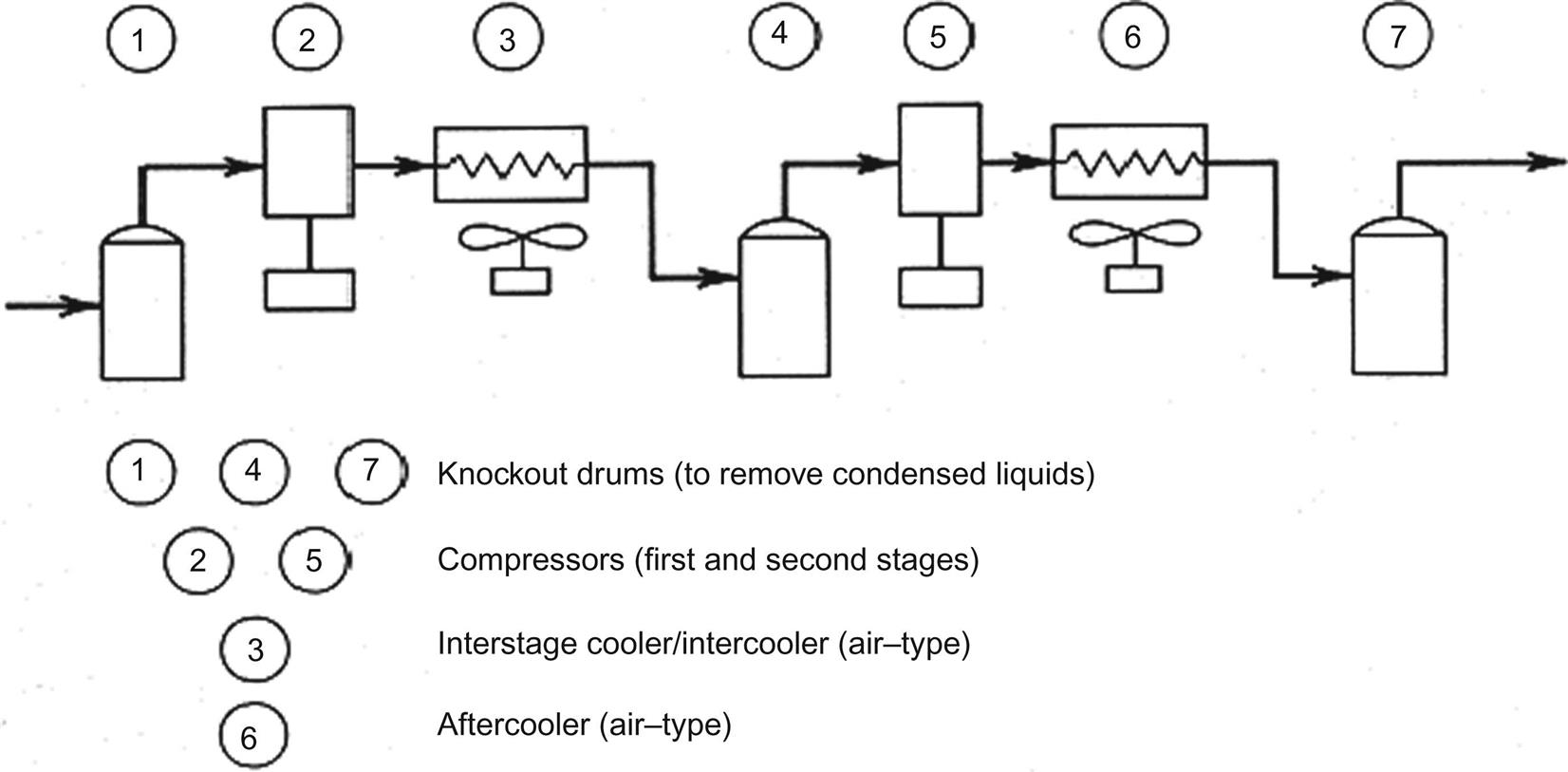
It will be shown later that the efficiency of compression drops with increased compression ratio p₂/p₁. Most field applications require multistage compressors (two, three, and sometimes four stages) to reduce compression ratio in each stage. Fig. 11.6 shows a two-stage compression unit. Using compressor stages with perfect intercooling between stages gives a theoretical minimum power for gas compression. To obtain this minimum power, the compression ratio in each stage must be the same and the cooling between each stage must bring the gas entering each stage to the same temperature.

The compression ratio in each stage should be less than six to increase compression efficiency. The equation to calculate stage-compression ratio is

$r_s={\left(\frac{P_{dis}}{P_{in}}\right)}^{1/n_s},$ (11.56)

(11.56)

where P_dis, P_in, and n_s are final discharge pressure, inlet pressure, and number of stages, respectively.

For a two-stage compression, the compression ratio for each stage should be

$r_s=\sqrt{\frac{P_{dis}}{P_{in}}}.$ (11.57)

(11.57)

Using Eq. (11.50), we can write the total power requirement for the two-stage compressor as

$\begin{array}{cc}{P}_{total}& =\frac{k}{k-1}{w}_{t}R{T}_{in1}\left[{\left({\displaystyle \frac{P_{dis1}}{P_{in1}}}\right)}^{\frac{k-1}{k}}-1\right]+\frac{k}{k-1}{w}_{t}R{T}_{in}2\left[{\left({\displaystyle \frac{P_{dis2}}{P_{in2}}}\right)}^{\frac{k-1}{k}}-1\right].\end{array}$ (11.58)

(11.58)

The ideal intercooler will cool the gas flow stage one to stage two to the temperature entering the compressor. Thus, we have T_in1=T_in2. Also, the pressure P_in2=P_dis1. Eq. (11.58) may be written as

$\begin{array}{cc}{P}_{total}& =\frac{k}{k-1}{w}_{t}R{T}_{in1}\left[{\left({\displaystyle \frac{P_{dis1}}{P_{in1}}}\right)}^{\frac{k-1}{k}}-1\right]+\frac{k}{k-1}{w}_{t}R{T}_{in1}\left[{\left({\displaystyle \frac{P_{dis2}}{P_{in2}}}\right)}^{\frac{k-1}{k}}-1\right].\end{array}$ (11.59)

(11.59)

We can find the value of P_dis1 that will minimize the power required, P_total. We take the derivative of Eq. (11.59) with respect to P_dis1 and set this equal to zero and solve for P_dis1. This gives

$P_{dis1}=\sqrt{P_{in1}{P}_{dis2}},$

which proves Eq. (11.57).

For the two-stage compressor, Eq. (11.59) can be rewritten as

$P_{total}=\frac{2k}{k-1}{w}_{t}R{T}_1\left[{\left(\frac{P_{dis2}}{P_{in1}}\right)}^{\frac{k-1}{2k}}-1\right].$ (11.60)

(11.60)

The ideal intercooling does not extend to the gas exiting the compressor. Gas exiting the compressor is governed by Eq. (11.41). Usually there is an adjustable after-cooler on a compressor that allows the operators to control the temperature of the exiting flow of gas. For greater number of stages, Eq. (11.60) can be written in field units as

$H{P}_t=\frac{n_s{p}_1{q}_1}{229.2}\frac{k}{(k-1)}\left[{\left(\frac{p_2}{p_1}\right)}^{\frac{k-1}{n_{S}k}}-1\right]$ (11.61)

(11.61)

or

$H{P}_t=\frac{181.79n_S{p}_b{T}_1{Q}_{MM}}{T_b}\frac{k}{(k-1)}\left[{\left(\frac{p_2}{p_1}\right)}^{\frac{k-1}{n_{S}k}}-1\right].$ (11.62)

(11.62)

In the above, p₁ (psia) is the intake pressure of the gas and p₂ (psia) is the outlet pressure of the compressor after the final stage, q₁ is the actual cfm of gas into the compressor, HP_t is the theoretical horsepower needed to compress the gas. This HP_t value has to be matched with a prime mover motor. The proceeding equations have been coded in the spreadsheet ReciprocatingCompressorPower.xls for quick calculations.

Reciprocating compressors have a clearance at the end of the piston. This clearance produces a volumetric efficiency e_v. The relation is given by

$e_v=0.96\left\{1-\epsilon \left[r_S^{\frac{1}{k}}-1\right]\right\},$ (11.63)

(11.63)

where ε is the clearance ratio defined as the clearance volume at the end of the piston stroke divided by the entire volume of the chamber (volume contacted by the gas in the cylinder). In addition, there is a mechanical efficiency e_m of the compressor and its prime mover. This results in two separate expressions for calculating the required HP_t for reciprocating compressors and rotary compressors. The required minimum input prime mover motor to practically operate the compressor (either reciprocating or rotary) is

$H{P}_{in}=\frac{H{P}_t}{e_v{e}_m},$ (11.64)

(11.64)

where e_v≈0.80–0.99 and e_m≈0.80–0.95 for reciprocating compressors, and e_v=1.0 and e_m≈0.70–0.75 for rotary compressors.

Eq. (11.64) stands for the input power required by the compressor, which is the minimum power to be provided by the prime mover. The prime movers usually have fixed power HP_p under normal operating conditions. The usable prime mover power ratio is

$PR=\frac{H{P}_{in}}{H{P}_p}.$ (11.65)

(11.65)

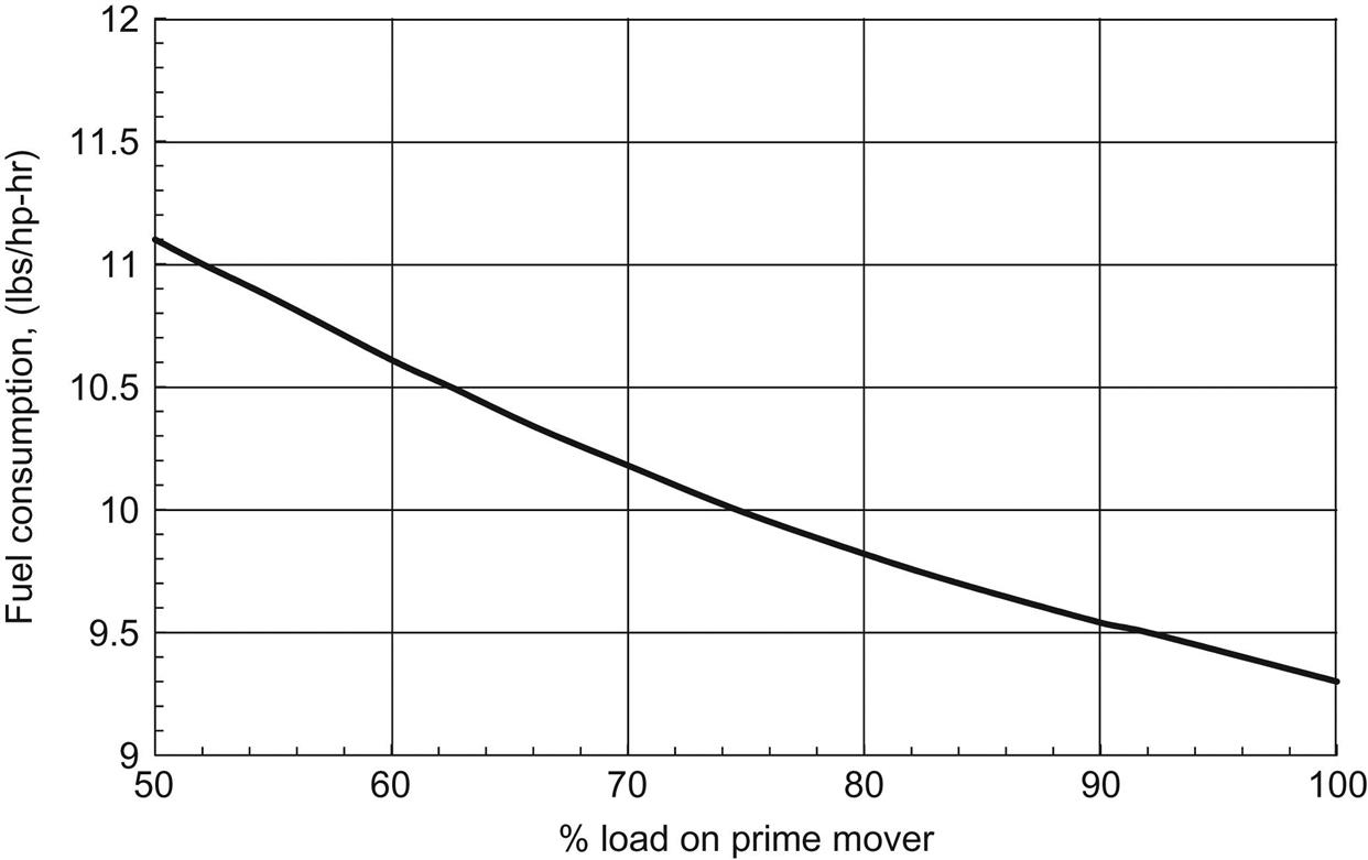
If the prime mover is not fully loaded by the compressor, its rotary speed increases and fuel consumption thus increases. Fig. 11.7 shows fuel consumption curves for prime movers using gasoline, propane/butane, and diesel as fuel. Fig. 11.8 presents fuel consumption curve for prime movers using natural gas as fuel. It is also important to know that the prime mover power drops with surface location elevation (Fig. 11.9).

ExampleProblem 11.2 Consider a three-stage reciprocating compressor that is rated at q=900 scfm and a maximum pressure capability of p_max=240 psig (standard conditions at sea level). The diesel prime mover is a diesel motor (naturally aspirated) rated at 300 horsepower (at sea-level conditions). The reciprocating compressor has a clearance ratio of ε=0.06 and e_m≈0.90. Determine the gallons/hr of fuel consumption if the working backpressure is 150 psig, and do for

Solution

1. Operating at sea level:

$\begin{array}{cc}{r}_s& =\sqrt[3]{\frac{p_{dis}}{p_{in}}}=\sqrt[3]{\frac{150+14.7}{14.7}}=\sqrt[3]{\frac{164.7}{14.7}}=\mathrm{2.2.4}\\ e_v& =0.96\left\{1-0.06\left[{(2.24)}^{\frac{1}{14}}-1\right]\right\}=0.9151\end{array}$

Required theoretical power to compress the gas:

$H{P}_t=(3)\frac{14.7(900)}{229.2}\left(\frac{1.4}{0.4}\right)\left[{\left(\frac{164.7}{14.7}\right)}^{\frac{0.4}{3,-(14)}}-1\right]=156.8\mathrm{hp}$

Required input power to the compressor:

$H{P}_r=\frac{H{P}_t}{e_m{e}_v}=\frac{156.8}{0.90(0.9151)}=190.3\mathrm{hp}$

Since the available power from the prime mover is 300 hp, which is greater than HP_r, the prime mover is okay. The power ratio is

$\mathrm{PR}=\frac{190.3}{300.0}=0.634\mathrm{or}63.4\%.$

From Fig. 11.7, fuel usage is approximately 0.56 lb/hp-hr. The weight of fuel requirement is, therefore,

$w_f(1b/\text{hr})\approx 0.56(190.3)=106.6\text{1b}/\text{hr}.$

The volumetric fuel requirement is

$q_f(\text{gallons}/\text{hr})\approx \frac{106.6}{6.9}=15.4\text{gallons}/\text{hr}.$

2. Operating at 6000 ft, the atmospheric pressure at an elevation of 6000 is about 11.8 psia (Lyons et al., 2001). Fig. 11.9 shows a power reduction of 22%.

$\begin{array}{ll}{r}_s\hfill & =\sqrt[3]{\frac{150+11.8}{11.8}}=2.39\hfill \\ e_v\hfill & =0.96\left\{1-0.06\left[{(2.39)}^{0.714}-1\right]\right\}=0.9013\hfill \end{array}$

$\begin{array}{ll}H{P}_t\hfill & =(3)\frac{11.8(900)}{229.2}\left(\frac{1.4}{0.4}\right)\left[{\left({\displaystyle \frac{161.8}{11.8}}\right)}^{0.0952}-2\right]=137.7\mathrm{hp}\hfill \\ H{P}_r\hfill & =\frac{137.7}{e_m{e}_v}=\frac{137.7}{0.90(0.9103)}=168.1\mathrm{hp}\hfill \\ H{P}_{in}\hfill & =300(1-0.22)=234\mathrm{hp}>168.1\mathrm{hp},\mathrm{so}\mathrm{okay}.\hfill \\ \mathrm{PR}\hfill & =\frac{161.8}{234}=0.718\mathrm{or}71.8\%\hfill \end{array}$

Fig. 11.7 shows that a fuel usage of 0.54 lb/hp-hr at 71.8% power ratio. Thus,

$\begin{array}{c}{w}_f(1\text{bs}/\text{hr})\approx 0.54(168.1)=90.81\text{bs}/\text{hr}\\ q_f(\text{gallons}/\text{hr})\approx \frac{90.8}{6.9}=13.2\text{gallons}/\text{hr}\end{array}$

11.3.3 Centrifugal Compressors

Although the adiabatic compression process can be assumed in centrifugal compression, polytropic compression process is commonly considered as the basis for comparing centrifugal compressor performance. The process is expressed as

$p{V}^n=\text{constastan},$ (11.66)

(11.66)

where n denotes the polytropic exponent. The isentropic exponent k applies to the ideal frictionless adiabatic process, while the polytropic exponent n applies to the actual process with heat transfer and friction. The n is related to k through polytropic efficiency E_p:

$\frac{n-1}{n}=\frac{k-1}{k}\times \frac{1}{E_p}.$ (11.67)

(11.67)

The polytropic efficiency of centrifugal compressors is nearly proportional to the logarithm of gas flow rate in the range of efficiency between 0.7 and 0.75. The polytropic efficiency chart presented by Rollins (1973) can be represented by the following correlation:

$E_p=0.61+0.03\log (q_1),$ (11.68)

(11.68)

where

q₁=gas capacity at the inlet condition, cfm.

There is a lower limit of gas flow rate, below which severe gas surge occurs in the compressor. This limit is called “surge limit.” The upper limit of gas flow rate is called “stone-wall limit,” which is controlled by compressor horsepower.

The procedure of preliminary calculations for selection of centrifugal compressors is summarized as follows:

1. Calculate compression ratio based on the inlet and discharge pressures:

$r=\frac{p_2}{p_1}$ (11.69)

(11.69)

2. Based on the required gas flow rate under standard condition (q), estimate the gas capacity at inlet condition (q₁) by ideal gas law:

$q_1=\frac{p_b}{p_1}\frac{T_1}{T_b}q$ (11.70)

(11.70)

3. Find a value for the polytropic efficiency E_p from the manufacturer's manual based on q₁.

4. Calculate polytropic ratio (n-1)/n using Eq. (11.67):

$R_p=\frac{n-1}{n}=\frac{k-1}{k}\times \frac{1}{E_p}$ (11.71)

(11.71)

5. Calculate discharge temperature by

$T_2=T_1{r}^{R_p}.$ (11.72)

(11.72)

6. Estimate gas compressibility factor values at inlet and discharge conditions.

7. Calculate gas capacity at the inlet condition (q₁) by real gas law:

$q_1=\frac{z_1{p}_b}{z_2{p}_1}\frac{T_1}{T_b}q$ (11.73)

(11.73)

8. Repeat Steps 2–7 until the value of q₁ converges within an acceptable deviation.

9. Calculate gas horsepower by

$H{p}_g=\frac{q_1{p}_1}{229E_p}\left(\frac{z_1+z_2}{2z_1}\right)\left(\frac{r^{R_p}-1}{R_p}\right),$ (11.74)

(11.74)

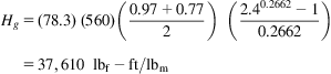
Some manufacturers present compressor specifications using polytropic head in lb_f-ft/lb_m defined as

$H_g=R{T}_1\left(\frac{z_1+z_2}{2}\right)\left(\frac{r^{R_p}-1}{R_p}\right),$ (11.75)

(11.75)

where R is the gas constant given by 1544/MW_a in psia-ft³/lb_m-°R. The polytropic head relates to the gas horsepower by

$H{p}_g=\frac{m_{t}Hg}{33,000E_p},$ (11.76)

(11.76)

where m_t is mass flow rate in lb_m/min.

10. Calculate gas horsepower by:

$H{p}_b=H{p}_g+\mathrm{\Delta }H{p}_m,$ (11.77)

(11.77)

where ΔHp_m is mechanical power losses, which is usually taken as 20 horsepower for bearing and 30 horsepower for seals.

The proceeding equations have been coded in the spreadsheet CentrifugalCompressorPower.xls for quick calculations.

Example Problem 11.3 Size a centrifugal compressor for the following given data:

Solution Calculate compression ratio based on the inlet and discharge pressures:

$r=\frac{600}{250}=2.4$

Calculate gas flow rate in scfm:

$q=\frac{144,000,000}{(24)(60)}=100,000\mathrm{scfm}$

Based on the required gas flow rate under standard condition (q), estimate the gas capacity at inlet condition (q₁) by ideal gas law:

$q_1=\frac{(14.7)}{(250)}\frac{(560)}{(520)}(100,000)=6332\mathrm{cfm}$

Find a value for the polytropic efficiency based on q₁:

$E_p=0.61+0.031\log (6332)=0.724$

Calculate polytropic ratio (n–1)/n:

$R_p=\frac{n-1}{n}=\frac{1.24-1}{1.24}\times \frac{1}{0.724}=0.2673$

Calculate discharge temperature:

$T_2=(560){(2.4)}^{0.2673}={707.7}^{\circ }\mathrm{R}={247.7}^{\circ }\mathrm{F}$

Estimate gas compressibility factor values at inlet and discharge conditions (spreadsheet program Hall-Yaborough-z.xls can be used):

$\begin{array}{ll}{z}_1\hfill & =0.97\mathrm{at}250\mathrm{psia}{\mathrm{and\; 100}}^{\circ }\mathrm{F}\hfill \\ z_2\hfill & =0.77\mathrm{at}600\mathrm{psia}\mathrm{and\; 247}{.7}^{\circ }\mathrm{F}\hfill \end{array}$

Calculate gas capacity at the inlet condition (q₁) by real gas law:

$q_1=\frac{(0.97)(14.7)}{(0.77)(250)}\frac{(560)}{(520)}(100,000)=7977\mathrm{cfm}$

Use the new value of q₁ to calculate E_p:

$E_p=0.61+0.03\log (7977)=0.727$

Calculate the new polytropic ratio (n–1)/n:

$R_p=\frac{n-1}{n}=\frac{1.24-1}{1.24}\times \frac{1}{0.727}=0.2662$

Calculate the new discharge temperature:

$T_2=(560){(2.4)}^{0.2662}={707}^{\circ }\mathrm{R}={247}^{\circ }\mathrm{F}$

Estimate the new gas compressibility factor value:

$z_2=0.77\mathrm{at}600\mathrm{psia}\mathrm{and}{247}^{\circ }\mathrm{F}$

Because z₂ did not change, q₁ remains the same value of 7977 cfm.

Calculate gas horsepower:

$\begin{array}{ll}H{p}_g\hfill & =\frac{(7977)(250)}{(229)(0.727)}\left(\frac{0.97+0.77}{2(0.97)}\right)\left(\frac{{2.4}^{0.2662}-1}{0.2662}\right)\hfill \\ \hfill & =10,592\mathrm{hp}\hfill \end{array}$

Calculate gas apparent molecular weight:

$M{W}_a=(0.68)(29)=19.72$

Calculated gas constant:

$R=\frac{1544}{19.72}=78.3\mathrm{psia}-{\mathrm{ft}}^3/1{\mathrm{b}}_{\mathrm{m}}{-}^{\circ }\mathrm{R}$

Calculate polytropic head:

$\begin{array}{ll}{H}_g\hfill & =(78.3)(560)\left(\frac{0.97+0.77}{2}\right)\left(\frac{{2.4}^{0.2662}-1}{0.2662}\right)\hfill \\ \hfill & =37,610{\mathrm{lb}}_{\mathrm{f}}-{\text{ft}/\text{lb}}_{\mathrm{m}}\hfill \end{array}$

Calculate gas horsepower requirement:

$H{p}_b=10,592+50=10,642\mathrm{hp}.$