
PID Admittance Control in Joint Space
Abstract
Normal impedance/admittance needs robot models. The model for the exoskeleton includes forward kinematic, inverse kinematic, and dynamic models. The kinematics are used to calculate the relation between the joint angles and the arm position, while the dynamic model is applied to design controllers. It is impossible to design a model-based impedance/admittance control when a complete dynamic model of the robot is unknown [154].
When the admittance control is in joint space, it requires inverse kinematics of the robot. In this chapter, the admittance control is modified to only use the orientations of the end-effector to generate the desired joint angles to avoid inverse kinematics. The classic PD control is also modified with adaptive compensation and sliding mode compensation. The stability of these two PD controllers are proven. Real time experiments are presented for with a 2-DoF pan and tilt robot and a 4-DoF exoskeleton. The experiment results show the effectiveness of the proposed controllers.
Keywords
PID control; Admittance control; Joint space
9.1 PD admittance control
The dynamics of a n-link robot is
where ![]() represents the link positions.
represents the link positions. ![]() is the inertia matrix,
is the inertia matrix, ![]() represents centrifugal and Coriolis matrix,
represents centrifugal and Coriolis matrix, ![]() is vector of gravitational torques,
is vector of gravitational torques, ![]() denotes the joint driving torque,
denotes the joint driving torque, ![]() is the Jacobian matrix,
is the Jacobian matrix, ![]() represents the contact force and torque in the end-effector.
represents the contact force and torque in the end-effector.
When the robot dynamic (9.1) is known, the traditional admittance control is
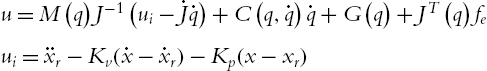
where ![]() denote the gains of the proportional and derivative (PD) controller.
denote the gains of the proportional and derivative (PD) controller.
For the human–robot cooperation, we assume the end-effector of the robot does not have contact with the environment, ![]() . This traditional admittance controller enhances robustness against the modeling error by using an inner position loop. However, the inner loop dynamics hinder accurate realization of desired admittance dynamics.
. This traditional admittance controller enhances robustness against the modeling error by using an inner position loop. However, the inner loop dynamics hinder accurate realization of desired admittance dynamics.
Since ![]() is the desired reference in the task space, it should be transformed into joint space as the desired angles
is the desired reference in the task space, it should be transformed into joint space as the desired angles ![]() :
:

where ![]() is the inverse kinematic of the robot (9.1).
is the inverse kinematic of the robot (9.1).
We apply the output of the forces/torques sensor to the admittance model, and generate desired angles in joint space:

1-DoF robot
We can use one force to move any Cartesian position without the inverse kinematics. For more than one DoF, the relation between different forces are coupled, then the inverse kinematics are needed.
We propose a simplified admittance control, which does not need ![]() . The basic idea is that we establish the relation between the orientation of the robot and the force/torque. We use the torques instead of the forces, because the orientation is a linear combination of the joint angles.
. The basic idea is that we establish the relation between the orientation of the robot and the force/torque. We use the torques instead of the forces, because the orientation is a linear combination of the joint angles.
The orientations are practically decoupled in most of the cases. Even the orientations are coupled, we show in the following that the orientations are linear combinations of the robot joint angles.
2-DoF robot
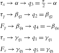
A typical 2-DoF robot is the pan and tilt robot shown in Fig. 9.1. A six-axis force and torque sensor is used by the operator outside the manipulator. It measures the full six components of force and torque: vertical, lateral, and longitudinal forces as well as camber, steer, and torque movements. For the 2-DoF robot, we only use two of them.

To simplify the model, we assume that the links are thin and symmetric bars. Therefore the center of mass of each link is in its center. The orientations of the robot are defined as α, β, and γ, and they can be calculated directly from geometrical property:

So the orientation of the robot is completely defined by the joint angles of the robot. The admittance control (9.2) generates three orientations and three positions in the task space. Two orientations in (9.5) can generate two desired angles on the robot in the joint space.
The Jacobian for the 2-DoF robot only includes the orientational components as

One advantage of (9.6) is that we do not need the kinematics of the robot.
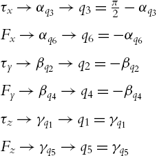
4-DoF robot
A typical 4-DoF robot is shown in Fig. 9.2. As the pan and tilt robot, the links are also assumed to be thin and symmetric. The orientation of the robot is:

The orientation in (9.7) has a linear combination of the robot joints at the β orientation. We cannot use only the angular component in the Jacobian ![]() , because the determinant would be zero. To avoid the singularity, we divided the orientation β in two terms:
, because the determinant would be zero. To avoid the singularity, we divided the orientation β in two terms:

Because the torques can form the joint positions, we can use both torque and force at the Y direction to generate ![]() and
and ![]() . This consideration is possible because the joint number is less than the Cartesian DoF, and there are still force components that can be used.
. This consideration is possible because the joint number is less than the Cartesian DoF, and there are still force components that can be used.

The force/torque transformation to joint position are

It is a one-to-one mapping from the force/torque to joint angles.
5-DoF robot
The orientation for a 5-DoF robot is:

Now the γ orientation has a linear combination.
Because the DoF of the robot n and the DoF of the force/torque sensor m satisfy
we can separate the orientations in two terms and use the force components to calculate one of them:
6-DoF robot
For a 6-DoF robot, ![]() , the orientations are
, the orientations are

All orientations have linear combinations of the joint angles. It is still possible to divide them in two terms, and use the force components as
Since α orientation has a constant value, we can establish the division for it. The desired reference angles are ![]() .
.
Generally, the orientations of 2-DoF robot are defined by each joint of the robot, and we can apply the torques in certain directions directly. For more than three DoF robots, the orientations of the robot are defined by multiple joints. If the DoF of the robot is less than the DoF of the force/torque sensor, we can divide the force and torque components into the orientations. If the robot is redundant, i.e., ![]() ,
, ![]() , we have to make certain assumptions in joint movement, such as limiting the range of motion or fix the joint.
, we have to make certain assumptions in joint movement, such as limiting the range of motion or fix the joint.
9.2 PD admittance control with adaptive compensations
After the desired reference angle ![]() is obtained from the admittance control, we use PD control with compensations to control each joint. We define the tracking nominal error, Ω, as follows:
is obtained from the admittance control, we use PD control with compensations to control each joint. We define the tracking nominal error, Ω, as follows:
where ![]() denote the partial-proportional matrix gain. When
denote the partial-proportional matrix gain. When ![]() , the robot dynamics (9.1) can be linearly parameterized as
, the robot dynamics (9.1) can be linearly parameterized as
where ![]() is a regressor composed of known nonlinear functions, and
is a regressor composed of known nonlinear functions, and ![]() is a vector which represents unknown but constant parameters.
is a vector which represents unknown but constant parameters.
The dynamics parametrization can be written in terms of a nominal reference ![]() and its derivative
and its derivative ![]() , as follows:
, as follows:
where ![]() is the regressor in terms of the nominal reference
is the regressor in terms of the nominal reference ![]() .
.
The following properties will be used to prove stability:
1) The inertia matrix ![]() is symmetric positive definite, and there exists a number
is symmetric positive definite, and there exists a number ![]() such that
such that
where ![]() and
and ![]() are the maximum and minimum eigenvalues of the matrix A. The norm
are the maximum and minimum eigenvalues of the matrix A. The norm ![]() stands for the induced Frobenius norm.
stands for the induced Frobenius norm.
2) For the centripetal and Coriolis matrix ![]() , there exists a number
, there exists a number ![]() such that
such that
and ![]() is skew-symmetric, i.e.,
is skew-symmetric, i.e.,
The norm ![]() of the vector
of the vector ![]() stands for the vector Euclidean norm.
stands for the vector Euclidean norm.
3) For the gravitational torques vector ![]() , there exists a number
, there exists a number ![]() such that
such that
4) For the Jacobian ![]() , and the time derivative of the Jacobian
, and the time derivative of the Jacobian ![]() , there exist numbers
, there exist numbers ![]() (
(![]() ) such that
) such that

When M, C, and G are unknown, (9.15) can be written in the adaptive form:
where ![]() and
and ![]() are estimates of
are estimates of ![]() , and Θ, respectively.
, and Θ, respectively.
We use the following PD control with adaptive compensation for each joint control:
where ![]() denote the matrix gain of the controller.
denote the matrix gain of the controller.
The closed-loop system with the controller (9.21) is
The product of the regressor ![]() with the parameter error vector
with the parameter error vector ![]() is
is
where ![]() , and
, and ![]() .
.
Since the PD controller ![]() can cancel the uncertainties of
can cancel the uncertainties of ![]() and
and ![]() , we only estimate the gravitational torque vector
, we only estimate the gravitational torque vector ![]() , then the closed-loop system (9.22) becomes
, then the closed-loop system (9.22) becomes

Here, the product of the regressor is divided in two terms, the first term ![]() corresponds to the gravity torque vector estimation, the second term
corresponds to the gravity torque vector estimation, the second term ![]() corresponds to the inertia and Coriolis matrices,
corresponds to the inertia and Coriolis matrices, ![]() ,
, ![]() .
.
Theorem 9.1
Proof
We proposed the following Lyapunov function:
The first term corresponds to the kinetic energy of the closed-loop system, the second term is the adaptive term and ![]() denote its matrix gain. Taking the time derivative of (9.27) along (9.24), gives rise to
denote its matrix gain. Taking the time derivative of (9.27) along (9.24), gives rise to
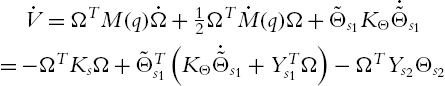
From (9.28) if the adaptation law is (9.26) the time derivative of V reduces to

Using the properties (9.16), (9.17), and (9.19) on ![]() becomes
becomes
where ![]() is a state dependent function. Therefore
is a state dependent function. Therefore ![]() is
is
That implies that there exists a large enough gain ![]() such that
such that ![]() and the nominal error converges into a set-bounded
and the nominal error converges into a set-bounded ![]() as
as ![]() ; and by the Barbalat lemma the time derivative of the vector parameters error
; and by the Barbalat lemma the time derivative of the vector parameters error ![]() converge into a set-bounded ϵ when
converge into a set-bounded ϵ when ![]() as
as ![]() . □
. □
9.3 PD admittance control with sliding mode compensations
The PD control with adaptive compensation (9.21) is still complex. Now we use a more simple compensator, sliding mode control, to compensate the PD control. The PD control with sliding mode compensation for each joint control is

where ![]() is the sliding mode matrix gain,
is the sliding mode matrix gain, ![]() . It is the second-order sliding mode.
. It is the second-order sliding mode.
The robot dynamics (9.1) with the controller (9.30) gives the closed-loop system as
Theorem 9.2
Proof
We proposed the following Lyapunov function:
Taking the time derivative of (9.31) gives rise to

Using the properties (9.16) and (9.19) on ![]() become
become
where υ is a state dependent function bigger than χ in the adaptive compensation Therefore ![]() is
is
That implies that there exists a large enough gain ![]() such that
such that ![]() and the nominal error converges into a set-bounded
and the nominal error converges into a set-bounded ![]() as
as ![]() . □
. □
9.4 PID admittance control
The PID control structure is similar as the previous controller. The control law is

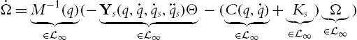
The closed-loop system of the model (9.24) under the control law (9.33) is
The regressor is bounded by

Let us consider the following Lyapunov function candidate:
that corresponds to the kinetic energy of the manipulator in closed loop. The time derivative of V along of (9.34) is

Using dynamics properties, the above expression reduces to
In order for ![]() to be negative definite, it needs
to be negative definite, it needs
that indicates that there exists a big enough ![]() such that
such that ![]() . Even more, we have the following:
. Even more, we have the following:
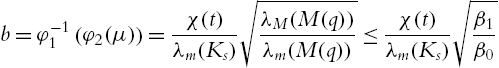
it is defined ![]() and
and ![]() . The ultimate bound is
. The ultimate bound is
that implies that Ω is bounded by

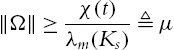
Finally, we can conclude that the solutions of Ω are ultimately uniformly bounded. If it is considered that we have a big enough gain ![]() such that
such that ![]() ,
, ![]() can be written as
can be written as
As in the previous controller, the nominal error ![]() and
and ![]() because it is bounded and does not grow over the time. From (9.34), it is observed that
because it is bounded and does not grow over the time. From (9.34), it is observed that
that implies ![]() and, therefore, from Barbalat's lemma, Ω converges into a ball of radio μ when
and, therefore, from Barbalat's lemma, Ω converges into a ball of radio μ when ![]() .
.
Consider the following Cartesian nominal reference:

![]() is the sliding surface that depends on the Cartesian error and its derivative.
is the sliding surface that depends on the Cartesian error and its derivative.
The function ![]() corresponds to the discontinuous function sign of
corresponds to the discontinuous function sign of ![]() . The control law is given by
. The control law is given by

The Cartesian nominal reference is bounded by

The system in closed-loop and its stability analysis is the same as the PID admittance control of the previous section.
9.5 Experimental results
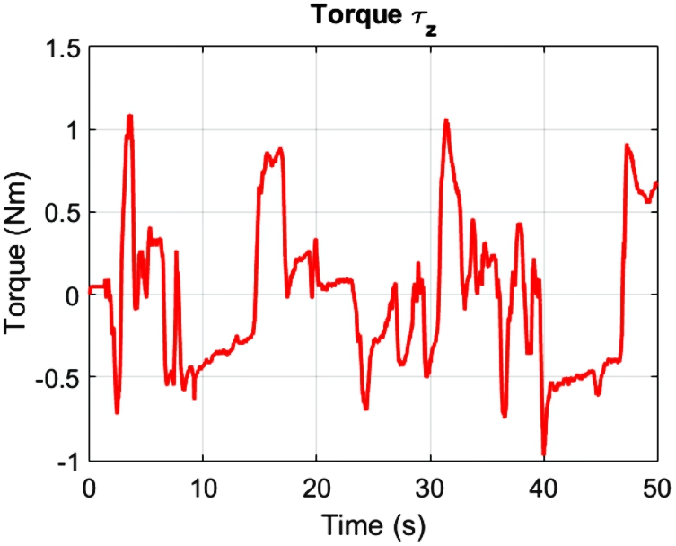
We use two robots to test our stable PD admittance control. The 2-DoF pan and tilt robot shown in Fig. 9.1. The force/torque (F/T) sensor is the 6-DoF Schunk®. Another robot is a 4-DoF exoskeleton robot; see Fig. 9.2. The real time control environment is Simulink and Matlab 2012. The communication is the CAN protocol, which enables the PC to communicate with the actuators and the F/T sensor.
9.5.1 Pan and tilt robot
The parameters of the PD control are given in Table 9.1. Here, diag![]() denotes a diagonal matrix of
denotes a diagonal matrix of ![]() with diagonal values val. (See also Figs. 9.3–9.6.)
with diagonal values val. (See also Figs. 9.3–9.6.)
Table 9.1
The parameters of PD control
| Gain | Classic PD | Adaptive PD | Sliding PD |
|---|---|---|---|
| K p | diag |
– | – |
| K D | diag{100}2×2 | – | – |
| Λ | – | diag |
|
| K m | – | – | diag{0.15}2×2 |
| K Θ | – | 1 × 10⁻³ | – |
| K s | – | diag |
|


9.5.2 4-DoF exoskeleton
In this application the human–machine interface is a 6-axis force/torque sensor, Mini40 F/T Sensor (ATI Industrial Automation). This sensor system includes a data acquisition system. It sends digital signals of three forces and three torques to the computer via the RS232 serial port. The reference signals are generated by (9.5). We choose ![]() ,
, ![]() ,
, ![]() . For the 4-DoF exoskeleton, the parameters for the PD controllers are given in the Table 9.2.
. For the 4-DoF exoskeleton, the parameters for the PD controllers are given in the Table 9.2.
Table 9.2
The parameters of PD control
| Gain | Traditional PD | Adaptive PD | Sliding PD |
|---|---|---|---|
| K p | diag |
– | – |
| K d | diag{10}4×4 | – | – |
| Λ | – | diag |
|
| K m | – | – | diag{1}4×4 |
| K Θ | – | diag{0.1}2×2 | – |
| K s | – | diag{3}4×4 | diag{2}4×4 |

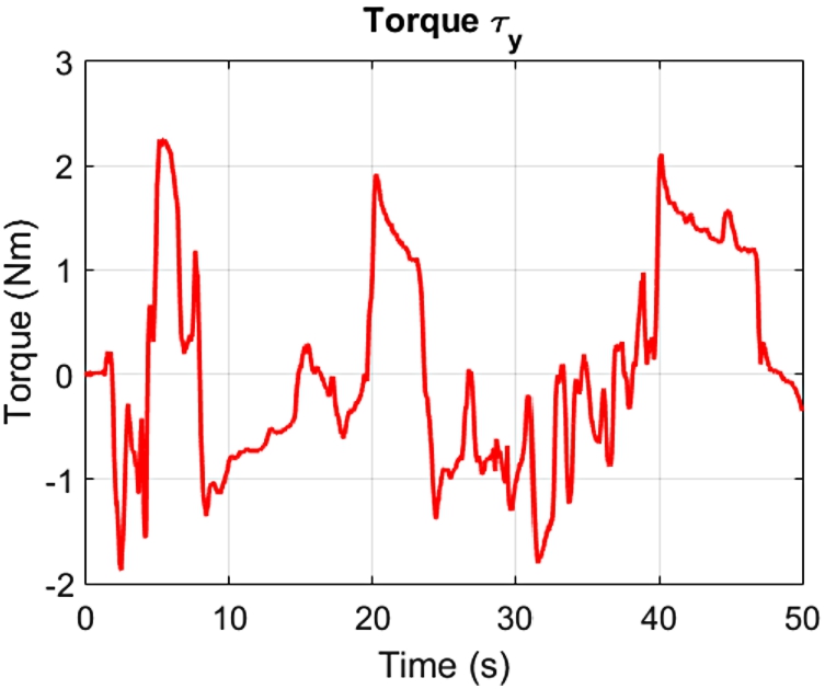
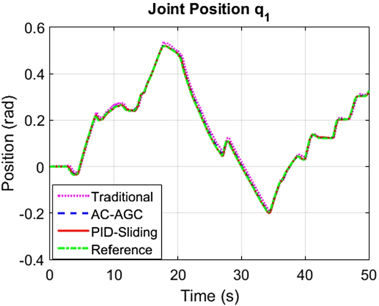
The admittance model is the same as above, with ![]() . We only present the flexion-extension results of the shoulder and the elbow. The results are given in Figs. 9.7–9.10.
. We only present the flexion-extension results of the shoulder and the elbow. The results are given in Figs. 9.7–9.10.


The results show that the PD admittance control with compensations is better than the traditional controller. The proposed PD admittance controllers present high precision tracking despite the presence of gravitational terms.
9.6 Conclusion
In this chapter, novel admittance controllers are presented, which work in joint space. They do not need the inverse kinematics of the robot. These PD and PID controllers use adaptive and sliding mode compensations to improve the tracking accuracy. Stability of the controllers are proven via Lyapunov analysis. The proposed controllers are verified using a 2-DoF pan and tilt robot and a 4-DoF exoskeleton with a F/T sensor. The comparisons between traditional and proposed controllers are made.