
Stable PID Control and Systematic Tuning of PID Gains
Abstract
Although great progress has been made in a century-long effort to design and implement robotic exoskeletons, many design challenges continue to limit the performance of the system. One of the limiting factors is the lack of simple and effective control systems for the exoskeleton [56,137]. The position error caused by gravitational torques can be reduced by introducing an integral component to the PD control. In order to assure asymptotic stability, several components were previously added to the classic linear PID controllers, for example, fourth-order filter [101], nonlinear derivative term [4], nonlinear integral term (saturated function) [71], input saturation, and nonlinear observer [2].
Linear PID is the simplest and the most popular industrial controller, since tuning its internal parameters does not require a model of the plant and can be performed experimentally. Lyapunov function was previously used for the tuning procedure of a linear PID [72]. However, the inertia matrix and the gravitational torque vector of the system have to be clearly defined [63,73]. If the robot dynamic can be rewritten into a decoupled linear system with bounded nonlinear system, the stability of linear PID can be proven [117]. The asymptotic stability was not achieved.
In this chapter, the semiglobal asymptotic stability is proven along with a new approach for tuning the parameters of the PID controller. We apply this method on an upper limb exoskeleton. Experimental results show that this new PID tuning method is simple, systematic, and effective for robot control.
Keywords
Semiglobal asymptotic stability; PID gains; Systematic tuning
2.1 Stable PD and PID control for exoskeleton robots
The dynamics of a serial n-link exoskeleton robot can be written as [131]
M(q)⋅⋅q+C(q,⋅q)⋅q+g(q)+f(⋅q)=τ
where q∈ℜn![]() denotes the joint positions, ⋅q∈ℜn
denotes the joint positions, ⋅q∈ℜn![]() denotes the joint velocities, M(q)∈ℜn×n
denotes the joint velocities, M(q)∈ℜn×n![]() is the inertia matrix, C(q,⋅q)∈ℜn×n
is the inertia matrix, C(q,⋅q)∈ℜn×n![]() is the centripetal and Coriolis matrix, f∈Rn
is the centripetal and Coriolis matrix, f∈Rn![]() is the frictional terms (Coulomb friction), τ∈ℜn
is the frictional terms (Coulomb friction), τ∈ℜn![]() is the input control vector, and g(q)∈ℜn
is the input control vector, and g(q)∈ℜn![]() is the gravity vector, which satisfies
is the gravity vector, which satisfies
g(q)=∂∂qU(q)U=∑ni=1mighi
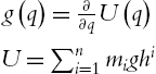
where hi=yi![]() , yi
, yi![]() is in the vector oi=[xi,yi,zi]T
is in the vector oi=[xi,yi,zi]T![]() , oi
, oi![]() is given by the first three elements of the fourth column of the homogeneous transformation matrix.
is given by the first three elements of the fourth column of the homogeneous transformation matrix.
The robot (2.1) has the following structural properties, which will be used in the stability analysis of the PID control.
Property 2.1. The inertia matrix is symmetric and positive definite, i.e.,
m1‖x‖2⩽xTMx⩽m2‖x‖2
where ∀x∈Rn![]() , m1
, m1![]() and m2
and m2![]() are known positive scalar constant, and ‖.‖
are known positive scalar constant, and ‖.‖![]() denotes the Euclidean vector norm.
denotes the Euclidean vector norm.
Property 2.2. The centripetal and Coriolis matrix is skew-symmetric, i.e.,
xT[⋅M(q)−2C(q,⋅q)]x=0

‖C(q,˙q)˙q‖⩽kc‖˙q‖2,kc>0
˙M(q)=C(q,˙q)+C(q,˙q)T
where Ck,ij(q)=(∂Bij∂qk+∂Bik∂qj−∂Bjk∂qi)![]() , kc=12maxq∈Rnn∑k=1‖Ck(q)‖
, kc=12maxq∈Rnn∑k=1‖Ck(q)‖![]() , and C0(q)
, and C0(q)![]() is a bounded matrix.
is a bounded matrix.
Property 2.3. The gravitational torques vector g(q)![]() in (2.2) is Lipschitz:
in (2.2) is Lipschitz:
‖g(x)−g(y)‖⩽kg‖x−y‖
The classic industrial PD law for the robot (2.1) is
τ=−Kp(q−qd)−Kd(⋅q−⋅qd)=PD1
where Kp In regulation case, the desired position is constant, ⋅qd=0
VPD=12˙qTM˙q+12˜qTKp˜q
where ˜q=q−qd By the property ˙qT[⋅M(q)−2C(q,⋅q)]˙q=0
XTY+YTX⩽XTΛX+YTΛ−1Y,
which is valid for any X, Y∈Rn×m
˙qT(G+F)⩽˙qTK1˙q+(G+F)TK−11(G+F)
where K1
⋅VPD=−˙qTKd˙q+˙qT(G+F)⩽−˙qT(Kd−K1)˙q+ˉd
where (g+f)TK−11(g+f)⩽ˉd
⋅VPD⩽−˙qT(Kd−K1)˙q
τ=−Kp(q−qd)−Kd(⋅q−⋅qd)+F+G
⋅VPD⩽−˙qT(Kd−K1)˙q
In tracking the case, the purpose is to make the joint motors follow the desired positions. The desired joint positions are generated by the path planning or trajectory planning, and are sent to the joint motors [72]. The tracking control can be divided into several regulations by the path planning. We can also use the following auxiliary error method. We define x1=q
‾x1=x1−xd1‾x2=˙x1−˙xd1ddt‾x1=‾x2
where xd1
r=‾x2+Λ‾x1
where Λ=ΛT>0
τ=−Kvr
When the dynamics of the robot (2.1) are known, the PD control with the known model compensation is
τ=−Kvr−f+(G+F)
where f=M(Λ⋅‾x1−⋅⋅qd)+C(Λ‾x1−⋅qd) We use the Lyapunov function candidate as
V=12rTMr
From Property 2.2, rT[⋅M−2C]r=0
⋅V=−rTKvr
Then r→0
⋅V⩽−rTKvr+ˉd
In general, the regulation error of the PD control law (2.7) is bounded in a ball with radius ˉd The stability property is not enough for robot control. The steady-state error caused by gravity and friction may be big. The derived gain Kd We use the stability property of PD control (2.7) to stabilize the open loop unstable robot (2.1). For any Kd>K1
M(q)⋅⋅q+C(q,⋅q)⋅q+g(q)+f(⋅q)=PD1
when the robot dynamics contain the gravitational torques vector g(q)
τ=PD1+ˆg(q)
where g(q)=ˆg(q)+˜g(q)
⋅VPD⩽−˙qT(Kd−K1)˙q+ˉd1
where ˉd1
M(q)⋅⋅q+C(q,⋅q)⋅q+g(q)+f(⋅q)=PD1+ˆg(q)
Similar stability results as before can be obtained and only the upper bound of the gravity becomes smaller. The position control objective is to evaluate the torque applied to the joints so that the robot joint displacements tend asymptotically to constant desired joint positions. Given a desired constant position qd∈Rn
˜q=qd−q
˜q→0
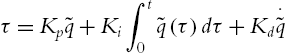
τ=Kp˜q+Ki∫t0˜q(τ)dτ+Kd⋅˜q
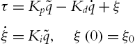
where Kp The common linear PID control does not include any component of the robot dynamics into its control law. In order to assure asymptotic stability of PID control, the simplest approach is to modify the linear PID into a nonlinear one. This chapter will work on the linear PID, which is the most popular industrial controller. In [117] the robot dynamic was rewritten in a decoupled linear system and bounded nonlinear system; this linear PID control could not guarantee asymptotic stability. Sufficient conditions of the linear PID in [72] were given via Lyapunov analysis. However, these conditions are not explicit; the PID gains could not be decided with these conditions directly, and a complex tuning procedure was needed [73]. Because ˙qd=0
τ=Kp˜q−Kd˙q+ξ˙ξ=Ki˜q,ξ(0)=ξ0
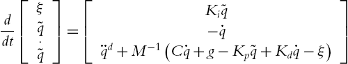
In matrix form, it is
ddt[ξ˜q⋅˜q]=[Ki˜q−˙q¨qd+M−1(C˙q+g−Kp˜q+Kd˙q−ξ)]
The closed-loop system of the robot (2.13) is
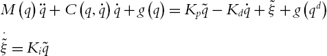
M(q)¨q+C(q,˙q)˙q+g(q)=Kp˜q−Kd˙q+ξ,˙ξ=Ki˜q
The equilibrium is [ξ,˜q,⋅˜q]=[ξ⁎,0,0]
M(q)¨q+C(q,˙q)˙q+g(q)=Kp˜q−Kd˙q+˜ξ+g(qd)⋅˜ξ=Ki˜q
Theorem 2.1 Consider the robot dynamic (2.1) controlled by the linear PID controller (2.16). The closed-loop system (2.18) is semiglobally asymptotically stable at the equilibrium x=[ξ−g(qd),˜q,⋅˜q]T=0
λm(Kp)⩾32kgλM(Ki)⩽βλm(Kp)λM(M)λm(Kd)⩾β+λM(M)
where β=√λm(M)λm(Kp)3
Proof We construct a Lyapunov function as
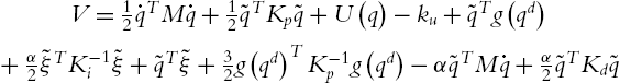
V=12˙qTM˙q+12˜qTKp˜q+U(q)−ku+˜qTg(qd)+α2˜ξTK−1i˜ξ+˜qT˜ξ+32g(qd)TK−1pg(qd)−α˜qTM˙q+α2˜qTKd˜q
where ku=minq{U(q)}
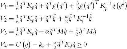
V1=16˜qTKp˜q+˜qTg(qd)+32g(qd)TK−1pg(qd)V2=16˜qTKp˜q+˜qT˜ξ+α2˜ξTK−1i˜ξV3=16˜qTKp˜q−α˜qTM˙q+12˙qTM˙qV4=U(q)−ku+α2˜qTKd˜q⩾0
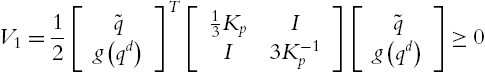
It is easy to find
V1=12[˜qg(qd)]T[13KpII3K−1p][˜qg(qd)]⩾0
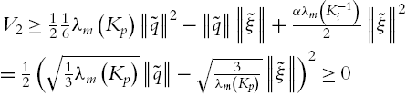
When α⩾3λm(K−1i)λm(Kp)
V2⩾1216λm(Kp)‖˜q‖2−‖˜q‖‖˜ξ‖+αλm(K−1i)2‖˜ξ‖2=12(√13λm(Kp)‖˜q‖−√3λm(Kp)‖˜ξ‖)2⩾0
Because
yTAx⩽‖y‖‖Ax‖⩽‖y‖‖A‖‖x‖⩽|λM(A)|‖y‖‖x‖
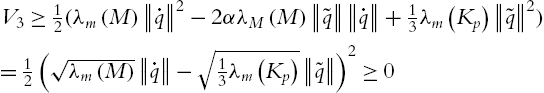
when α⩽√13λm(M)λm(Kp)λM(M)
V3⩾12(λm(M)‖˙q‖2−2αλM(M)‖˜q‖‖˙q‖+13λm(Kp)‖˜q‖2)=12(√λm(M)‖˙q‖−√13λm(Kp)‖˜q‖)2⩾0
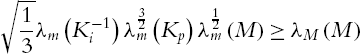
Obviously, if
√13λm(K−1i)λ32m(Kp)λ12m(M)⩾λM(M)
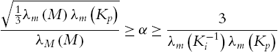
there exists
√13λm(M)λm(Kp)λM(M)⩾α⩾3λm(K−1i)λm(Kp)
This means if Kp
˙V=˙qTM¨q+12˙qT⋅M˙q+⋅˜qTKp˜q+g(q)T˙q+⋅˜qTg(qd)+⋅α˜ξTK−1i˜ξ+⋅˜qT˜ξ+˜qT⋅˜ξ−α(⋅˜qTM˙q+˜qT⋅M˙q+˜qTM¨q)−α˜qTKd˙q
Using (2.3), ddtU(q)=˙qTg(q)
−˙qTg(q)−˙qTKd˙q+˙qT˜ξ+˙qTg(qd)
Because ⋅˜qTg(qd)=−˙qTg(qd)
−˙qTKd˙q+α˜qT˜ξ+˜qTKi˜q
Now we discuss the last term of (2.23). From (2.5), we have
˜qT⋅M˙q=˜qTC˙q+˜qTCT˙q
From (2.1),
˜qTM¨q=−˜qTC˙q−˜qTg(q)+˜qTKp˜q−˜qTKd˙q+˜qT˜ξ+˜qTg(qd)
For the regulation case, ⋅˜qTM˙q=−˙qTM˙q
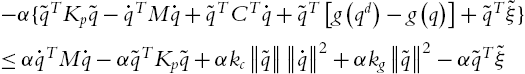
−α{˜qTKp˜q−˙qTM˙q+˜qTCT˙q+˜qT[g(qd)−g(q)]+˜qT˜ξ}⩽α˙qTM˙q−α˜qTKp˜q+αkc‖˜q‖‖˙q‖2+αkg‖˜q‖2−α˜qT˜ξ
˙V⩽−˙qT(Kd−αM−αkc‖˜q‖)˙q−˜qT(αKp−Ki−αkg)˜q⩽−[λm(Kd)−αλM(M)−αkc‖˜q‖]‖˙q‖2−[αλm(Kp)−λM(Ki)−αkg]‖˜q‖2
If
‖˜q‖⩽λM(M)αkc
and
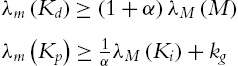
λm(Kd)⩾(1+α)λM(M)λm(Kp)⩾1αλM(Ki)+kg
then ˙V⩽0
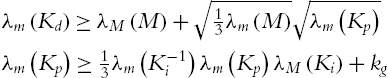
λm(Kd)⩾λM(M)+√13λm(M)√λm(Kp)λm(Kp)⩾13λm(K−1i)λm(Kp)λM(Ki)+kg
then (2.27) is established. Using (2.21) and λm(K−1i)=1λM(Ki) ˙V
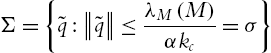
Σ={˜q:‖˜q‖⩽λM(M)αkc=σ}
˙V
Ω={x(t)=[˜q,˙q,˜ξ]∈R3n:˙V=0}={˜ξ∈Rn:˜q=0∈Rn,˙q=0∈Rn}
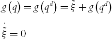
From (2.23), ˙V=0
g(q)=g(qd)=˜ξ+g(qd)⋅˜ξ=0
implies that ˜ξ=0 Finally, we conclude from all this that the origin of the closed-loop system (2.18) is locally asymptotically stable. Because 1α⩽λm(K−1i)λm(Kp)
˜q⩽λM(M)kcλM(Ki)λm(Kp)
It establishes the semiglobal stability of our controller, in the sense that the domain of attraction can be arbitrarily enlarged with a suitable choice of the gains. Namely, increasing Kp
Remark 2.1 From above stability analysis, we see the three gain matrices of the linear PID control (2.16) can be chosen directly from the conditions (2.19). The most important contribution of our method is the tuning procedure of the PID parameters can be calculated directly. It is more simple than the tuning procedures in [2,4,71–73,101,117]. No modeling information is needed. This linear PID control is exactly the same as the industrial robot controllers, and is semiglobally asymptotically stable. λM(M)
λM(M)⩽β,β⩾n(maxi,j|mij|)
2.1.1 Stable PD control
![]() and Kd
and Kd![]() are positive definite, symmetric, and constant matrices, which correspond to proportional and derivative coefficients, qd∈ℜn
are positive definite, symmetric, and constant matrices, which correspond to proportional and derivative coefficients, qd∈ℜn![]() is the desired joint position, ⋅qd∈ℜn
is the desired joint position, ⋅qd∈ℜn![]() is the desired joint velocity.
is the desired joint velocity.![]() . We use the Lyapunov function candidate as
. We use the Lyapunov function candidate as![]() .
.![]() and the matrix inequality [159]
and the matrix inequality [159]![]() and any 0<Λ=ΛT∈Rn×n
and any 0<Λ=ΛT∈Rn×n![]() , the modeling error ˙qT(G+F)
, the modeling error ˙qT(G+F)![]() can be estimated as
can be estimated as![]() is any positive definite matrix, the derivative of (2.8) is
is any positive definite matrix, the derivative of (2.8) is![]() , ˉd
, ˉd![]() can be regarded as upper bound of G+F
can be regarded as upper bound of G+F![]() .
.
![]() , ⋅VPD⩽0
, ⋅VPD⩽0![]() , the closed-loop system is stable.
, the closed-loop system is stable.![]() , the regulation error ˜q
, the regulation error ˜q![]() is bounded (stable), and ‖˙q‖(Kd−K1)
is bounded (stable), and ‖˙q‖(Kd−K1)![]() converges to ˉd
converges to ˉd![]() [54]
[54]
![]() , ⋅VPD⩽0
, ⋅VPD⩽0![]() , and the closed-loop system is stable.
, and the closed-loop system is stable.![]() as the link position vector, x2=˙q
as the link position vector, x2=˙q![]() as the link velocity vector. The tracking error is
as the link velocity vector. The tracking error is![]() is link position desired and xd2
is link position desired and xd2![]() is link velocity desired. The auxiliary error is defined as
is link velocity desired. The auxiliary error is defined as![]() . The PD control (2.7) becomes
. The PD control (2.7) becomes![]() .
.![]() ,
,![]() when the dynamics of the robot are known.
when the dynamics of the robot are known.![]() .
.![]() has to be increased to decrease them. In this way the closed-loop system becomes slow. This big settling time does not allow us to increase Kd
has to be increased to decrease them. In this way the closed-loop system becomes slow. This big settling time does not allow us to increase Kd![]() as we want.
as we want.![]() (K1>0
(K1>0![]() ), the following closed-loop system is stable:
), the following closed-loop system is stable:![]() . Gravity compensation is a popular method to modify the PD control (2.7). The new PD control is
. Gravity compensation is a popular method to modify the PD control (2.7). The new PD control is![]() , ˆg(q)
, ˆg(q)![]() , and ˜g(q)
, and ˜g(q)![]() are the gravity estimation and estimation error and in this case (2.9) become
are the gravity estimation and estimation error and in this case (2.9) become![]() is the upper bound of (˜g+f)
is the upper bound of (˜g+f)![]() , (˜g+f)TK−11(˜g+f)⩽ˉd1
, (˜g+f)TK−11(˜g+f)⩽ˉd1![]() . Normally, ˉd1<<ˉd
. Normally, ˉd1<<ˉd![]() , because ˜g
, because ˜g![]() is the estimation error of the gravity. The closed-loop system (2.13) becomes
is the estimation error of the gravity. The closed-loop system (2.13) becomes2.1.2 Stable PID control
![]() , semiglobal asymptotic stability of robot control is to design the input torque τ in (2.1) to cause regulation error
, semiglobal asymptotic stability of robot control is to design the input torque τ in (2.1) to cause regulation error![]() and ⋅˜q→0
and ⋅˜q→0![]() when initial conditions are in arbitrary large domain of attraction. Classic linear PID law is
when initial conditions are in arbitrary large domain of attraction. Classic linear PID law is![]() , Ki
, Ki![]() , and Kd
, and Kd![]() are proportional, integral, and derivative gains of the PID controller, respectively.
are proportional, integral, and derivative gains of the PID controller, respectively.![]() , ⋅˜q=−˙q
, ⋅˜q=−˙q![]() , the PID control law can be expressed via the following equations:
, the PID control law can be expressed via the following equations:![]() . Since at equilibrium point q=qd
. Since at equilibrium point q=qd![]() the equilibrium is [g(qd),0,0]
the equilibrium is [g(qd),0,0]![]() . In order to move the equilibrium to origin, we define ˜ξ=ξ−g(qd)
. In order to move the equilibrium to origin, we define ˜ξ=ξ−g(qd)![]() . The closed-loop equation becomes
. The closed-loop equation becomes![]() , provided that control gains satisfy
, provided that control gains satisfy![]() , kg
, kg![]() satisfies (2.6), λm(A)
satisfies (2.6), λm(A)![]() is the minimum eigenvalue of A, and λM(A)
is the minimum eigenvalue of A, and λM(A)![]() is the maximum eigenvalue of A.
is the maximum eigenvalue of A. ![]() , U(q)
, U(q)![]() is defined in (2.2), ku
is defined in (2.2), ku![]() is added such that V(0)=0
is added such that V(0)=0![]() . α is a design positive constant. We first prove V is a Lyapunov function, V⩾0
. α is a design positive constant. We first prove V is a Lyapunov function, V⩾0![]() . The term 12˜qTKp˜q
. The term 12˜qTKp˜q![]() is separated into three parts, and V=∑4i=1Vi
is separated into three parts, and V=∑4i=1Vi![]() :
:![]() ,
,![]() ,
,![]() is sufficiently large or Ki
is sufficiently large or Ki![]() is sufficiently small, (2.21) is established, and V(˙q,˜q,˜ξ)
is sufficiently small, (2.21) is established, and V(˙q,˜q,˜ξ)![]() is globally positive definite. Now we compute its derivative. Taking the derivative of V, we get
is globally positive definite. Now we compute its derivative. Taking the derivative of V, we get![]() , ddtg(qd)=0
, ddtg(qd)=0![]() , and ddt[˜qTg(qd)]=⋅˜qTg(qd)
, and ddt[˜qTg(qd)]=⋅˜qTg(qd)![]() , the first three terms of (2.23) become
, the first three terms of (2.23) become![]() and ⋅˜ξ=Ki˜q
and ⋅˜ξ=Ki˜q![]() , the first seven terms of (2.23) are
, the first seven terms of (2.23) are![]() , using (2.4) and (2.6) the last two terms of (2.23) are
, using (2.4) and (2.6) the last two terms of (2.23) are![]() , ‖˜q‖
, ‖˜q‖![]() decreases. From (2.22), if
decreases. From (2.22), if![]() , (2.28) is (2.19).
, (2.28) is (2.19).![]() is negative semidefinite. Define a ball Σ of radius σ>0
is negative semidefinite. Define a ball Σ of radius σ>0![]() centered at the origin of the state space, which satisfies these conditions:
centered at the origin of the state space, which satisfies these conditions:![]() is negative semidefinite on the ball Σ. There exists a ball Σ of radius σ>0
is negative semidefinite on the ball Σ. There exists a ball Σ of radius σ>0![]() centered at the origin of the state space on which ˙V⩽0
centered at the origin of the state space on which ˙V⩽0![]() . The origin of the closed-loop equation (2.18) is a stable equilibrium. Since the closed-loop equation is autonomous, we use LaSalle's theorem. Define Ω as
. The origin of the closed-loop equation (2.18) is a stable equilibrium. Since the closed-loop equation is autonomous, we use LaSalle's theorem. Define Ω as![]() if and only if ˜q=˙q=0
if and only if ˜q=˙q=0![]() . For a solution x(t)
. For a solution x(t)![]() to belong to Ω for all t⩾0
to belong to Ω for all t⩾0![]() , it is necessary and sufficient that ˜q=˙q=0
, it is necessary and sufficient that ˜q=˙q=0![]() for all t⩾0
for all t⩾0![]() . Therefore it must also hold that ¨q=0
. Therefore it must also hold that ¨q=0![]() for all t⩾0
for all t⩾0![]() . We conclude that from the closed-loop system (2.18), if x(t)∈Ω
. We conclude that from the closed-loop system (2.18), if x(t)∈Ω![]() for all t⩾0
for all t⩾0![]() , then
, then![]() for all t⩾0
for all t⩾0![]() . So x(t)=[˜q,˙q,˜ξ]=0∈R3n
. So x(t)=[˜q,˙q,˜ξ]=0∈R3n![]() is the only initial condition in Ω for which x(t)∈Ω
is the only initial condition in Ω for which x(t)∈Ω![]() for all t⩾0
for all t⩾0![]() .
.![]() , the upper bound for ‖˜q‖
, the upper bound for ‖˜q‖![]() can be
can be![]() the basin of attraction will grow. □
the basin of attraction will grow. □![]() can be estimated as [72]
can be estimated as [72]


2.2 PID parameters tuning in closed-loop
We use the following three important properties of robot PID control to derive a systematic tuning method:
- 1. In the regulation case, a robot can be stabilized by any PD controller providing their gains are positive big enough.
- 2. The closed-loop behaviors of robot PID control are similar with linear systems.
- 3. The control torque of each joint is independent of the robot dynamics.
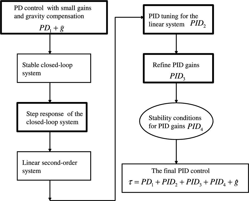
The turning steps are shown in Fig. 2.1. Here, PD1![]() is a PD controller, PID2
is a PD controller, PID2![]() is the PID controller after parameters tuning, PID3
is the PID controller after parameters tuning, PID3![]() is the PID controller after the parameters refining, and PID4
is the PID controller after the parameters refining, and PID4![]() is the PID controller after stability criterion. The final PID controller is τ.
is the PID controller after stability criterion. The final PID controller is τ.
Since the robot dynamic is not stable in an open loop, it is impossible to send step commands to all joints of the robot to tune PID gains. We use the following closed-loop tuning method.
The PD control (2.14) cannot guarantee zero of the steady-state error. The integrator is the most effective tool to eliminate steady-state error. PD control (2.7) becomes PID control as
τ=Kp˜q+Ki∫t0˜q(τ)dτ+Kdd˜qdt=PID2
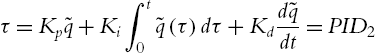
where Kp![]() , Ki
, Ki![]() , and Kd
, and Kd![]() are proportional, integral, and derivative gains of the PID controller, respectively. The integrator gain Ki
are proportional, integral, and derivative gains of the PID controller, respectively. The integrator gain Ki![]() has to be increased when the steady-state error is big. This causes big overshoot, long settling time, and is less robust. PD1
has to be increased when the steady-state error is big. This causes big overshoot, long settling time, and is less robust. PD1![]() is defined in (2.7) as
is defined in (2.7) as
PD1=−Kp(q−qd)−Kd(⋅q−⋅qd)
From (2.15), we know that any PD controller can guarantee stability (bounded) of any robot manipulator in the regulation case. The stability property assures us to find another PID controller for the closed-loop system as in Fig. 2.2A. The total control system is
τ=−Kp1(q−qd1)−Kd1(⋅q−⋅qd1)+ˆg(q)qd1=Kp2(q−qd)+Kd2(⋅q−⋅qd)Kp˜q+Ki∫t0(q−qd)dτ
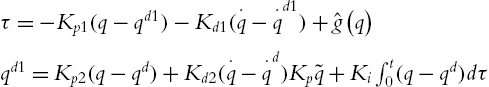

However, the controller (2.30) loses the PID form. Another tuning method in the closed-loop is to change PD1 directly; see Fig. 2.2B. Although the closed-loop system is different when PD1 is changed, the stability is always guaranteed with (2.15) with the change of PD1. The introduction of an integrator may destroy the stability, and in the next section we will show how to assure stability with PID control. We use Fig. 2.2B to adjust PID gains such that we can tune the PID controllers one by one.
Since PD/PID control is linear, the change of PD1 is the same as adding another controller PID2 to PD1. From (2.9), we know that the closed-loop system with PD1 is stable. When we apply a PID2 control to the closed-loop system (2.13), it is
M(q)⋅⋅q+C(q,⋅q)⋅q+˜g(q)+f(⋅q)−PD1=PID2
A gravity compensation to the closed-loop system (2.13) is
M(q)⋅⋅q+C(q,⋅q)⋅q+g(q)+f(⋅q)−PD1=ˆg(q)
When we apply the PID control and the gravity compensation to the closed-loop system (2.31), it is
M(q)⋅⋅q+C(q,⋅q)⋅q+g(q)+f(⋅q)−PD1=PID2+ˆg(q)
The total control torque to the robot is
τ=PID2+PD1+ˆg(q)
From (2.31) to (2.34), we see that the control torque to the robot manipulator is linearly independent of the robot dynamic (2.1). In the general case, if we tune PID controllers m times, they can be expressed as
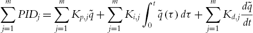
M(q)¨q+C(q,˙q)˙q+g(q)+f(⋅q)=m∑j=1PIDj+ˆg(q)
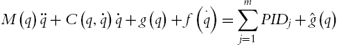
where
m∑j=1PIDj=m∑j=1Kp,j˜q+m∑j=1Ki,j∫t0˜q(τ)dτ+m∑j=1Kd,jd˜qdt
PD1 is a special PID with Ki=0![]() . This property allows us to start a PID control with small gains such that the closed-loop system is stable. Then any other tuning rule can be applied to obtain new PID gains one by one. The final PID gains are the summation of all these controllers (gains).
. This property allows us to start a PID control with small gains such that the closed-loop system is stable. Then any other tuning rule can be applied to obtain new PID gains one by one. The final PID gains are the summation of all these controllers (gains).
2.2.1 Linearization of the closed-loop system
Although the robot dynamics are strong nonlinear, the behaviors of the closed-loop system with PD/PID control are similar with the transient responses of a linear system. On the other hand, after PID control, each joint of the robot can be characterized as a single input–single output (SISO) system.
Several methods can be used to linearize the robot models. If the velocity and gravity are neglected, the terms C(q,˙q)˙q![]() and g(q)
and g(q)![]() in the nonlinear dynamics (2.1) are zero. The resulting system is a linear model [45]:
in the nonlinear dynamics (2.1) are zero. The resulting system is a linear model [45]:
M(q)¨q=u
Obviously, it is an oversimplified model. Since the velocity dependent term C(q,˙q)˙q![]() representing Coriolis-centrifugal forces, it is negligible for small joint velocities. A rate linearization scheme can be used as [44]
representing Coriolis-centrifugal forces, it is negligible for small joint velocities. A rate linearization scheme can be used as [44]
A¨q+Bq=u
where A=M(q)|q=q0![]() , B=∂g(q)∂q|q=q0
, B=∂g(q)∂q|q=q0![]() , q0
, q0![]() is an operating point. Many experiments show that even at low speeds, C(q,˙q)
is an operating point. Many experiments show that even at low speeds, C(q,˙q)![]() is not zero [127].
is not zero [127].
The velocity and gravity are main control issues of robots, and they are dominant components of the dynamics. When the robot model is completely known, Taylor series expansion can be applied [89]. At the operating point q0![]() the nonlinear model (2.1) can be approximated by
the nonlinear model (2.1) can be approximated by
A¨q+D˙q+Bq=τ
where A=M(q)|q=q0![]() , B=∂[g(q)+C(q,˙q)]∂q|q=q0
, B=∂[g(q)+C(q,˙q)]∂q|q=q0![]() , D=∂C(q,˙q)∂˙q|q=q0
, D=∂C(q,˙q)∂˙q|q=q0![]() .
.
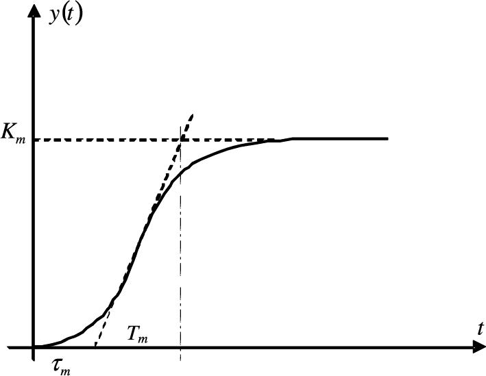
We use this identification-based linearization method. For each joint, the typical linear model is a first-order system with transportation delay as
Gp=Km1+Tmse−tms

The response is characterized by three parameters: the plant gain Km![]() , the delay time tm
, the delay time tm![]() , and the time constant Tm
, and the time constant Tm![]() . These are found by drawing a tangent to the step response at its point of inflection and noting its intersections with the time axis and the steady state value.
. These are found by drawing a tangent to the step response at its point of inflection and noting its intersections with the time axis and the steady state value.
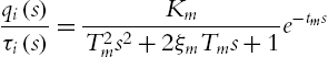
Sometimes the first-order (2.39) model cannot describe the complete nonlinear dynamic of the robot. A reasonable linear model of the robot is a Taylor series model as in (2.38). The model can be written in the frequency domain:
qi(s)τi(s)=KmT2ms2+2ξmTms+1e−tms
or
qi(s)τi(s)=Km(1+Tm1s)(1+Tm2s)e−tms
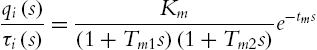
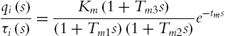
The responses of this second-order model are similar with mechanical motions. If there exists a big overshoot a negative zero is added in (2.40)
qi(s)τi(s)=Km(1+Tm3s)(1+Tm1s)(1+Tm2s)e−tms
The normal input signals for the PID tuning are step and repeat inputs.
2.2.2 PD/PID tuning
Because the robot can be approximated by a linear system, some tuning rules for linear systems can be applied for the closed-loop system tuning. We first give PD tuning rules. When each joint can be approximated by a first-order system,
Gp=Km1+Tmse−tms
Here, Km![]() , Tm
, Tm![]() , and tm
, and tm![]() are obtained from Fig. 2.3.
are obtained from Fig. 2.3.
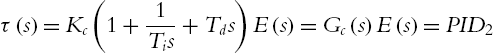
The linear PID law in time domain (2.29) can be transformed into the frequency domain:
τ(s)=Kc(1+1Tis+Tds)E(s)=Gc(s)E(s)=PID2
Similar with Ziegler–Nichols [161] and Cohen–Coon [20] tuning methods, we use a heuristic method to tune a PID controller. For PD control, our tuning law is shown in Table 2.1. Here, we use the similar tuning formulas with Ziegler–Nichols. By several experiments, we found a=1![]() is good.
is good.
Table 2.1
Ziegler–Nichols and Cohen–Coon methods for PI/PD
|
Kc
|
Ti
|
Td
|
|
|---|---|---|---|
| Ziegler–Nichols tuning |
aTmKmτm
|
0.5τm | |
| Cohen–Coon method |
TmKmτm(43+τm4Tm)
|
4Tmτm11Tm+2τm
|
|
| Our Method |
Tm2Km
|
T m1 |

If each joint is approximated by a second-order system,
qi(s)ui(s)=KmT2ms2+2ξmTms+1

The PD gains are tuned similarly with [58] and [24]; see Table 2.2.
Table 2.2
PD tuning for the second-order model
When PD control cannot provide good performances, PID control should be used. The PID gains for the first-order model is decided by Table 2.3.
Table 2.3
PID tuning for the first-order model
|
Kc
|
Ti
|
Td
|
|
|---|---|---|---|
| Ziegler–Nichols tuning | aTmKmτm |
2τm | 0.5τm |
| Cohen–Coon method |
TmKmτmτm4Tm
|
τm(32Tm+6τm)13Tm+8τm
|
4Tmτm11Tm+2τm
|
| Our Method |
Tm2Km
|
T m2 | T m1 |

Here, Kc=Kp![]() is a proportional gain, Ti=KcKi
is a proportional gain, Ti=KcKi![]() is a time constant, and Td=KdKc
is a time constant, and Td=KdKc![]() is a derivative time constant.
is a derivative time constant.
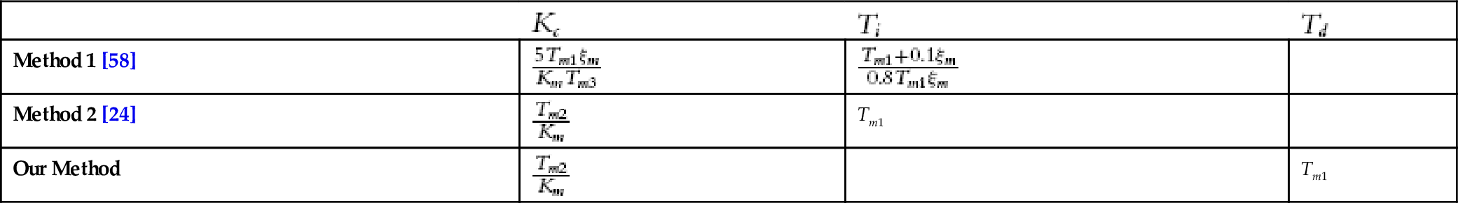
The PID gains for the second-order model is decided by Table 2.4.
Table 2.4
PID tuning for the second-order model
|
Kc
|
Ti
|
Td
|
|
|---|---|---|---|
| Method 1 |
5Tm1ξmKmTm3
|
2Tm1ξm |
Tm1+0.1ξm0.8Tm1ξm
|
| Method 2 |
Tm2Km
|
T m2 | T m1 |
| Our Method |
20ξmTmKm
|
15ξmTm |
T2m10
|

2.2.3 Refine PID gains
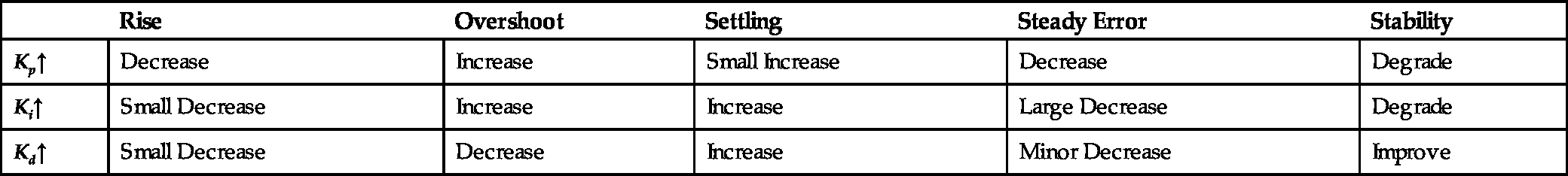
From (2.35), we see the PID gains are linear independent, and we can modify them directly. The refinement of PID2 is the same as adding a new PID controller, PID3, into (2.34). We use Table 2.5 to refine PID gains.
Table 2.5
Refined PID (PID3)
| Rise | Overshoot | Settling | Steady Error | Stability | |
|---|---|---|---|---|---|
| Kp↑ | Decrease | Increase | Small Increase | Decrease | Degrade |
| Ki↑ | Small Decrease | Increase | Increase | Large Decrease | Degrade |
| Kd↑ | Small Decrease | Decrease | Increase | Minor Decrease | Improve |
After we refine the process, the robot control is
τ=PD1+PID2+PID3+ˆg(q)
In order to decrease the steady-state error, we should increase Ki![]() . In order to get less settling time, we should decrease Kd
. In order to get less settling time, we should decrease Kd![]() . In order to get less overshoot, we should decrease Kp
. In order to get less overshoot, we should decrease Kp![]() . However, the above tuning process does not guarantee stability of the closed-loop system. In the next subsection, we will give the bounds of the PID gains to assure PID control is stable.
. However, the above tuning process does not guarantee stability of the closed-loop system. In the next subsection, we will give the bounds of the PID gains to assure PID control is stable.
2.2.4 Stability conditions for PID gains
For the robot dynamic controlled by the PID controller (2.35), the closed-loop system (2.18) is semiglobally asymptotically stable at the equilibrium x=[ξ−g(qd),˜q,⋅˜q]T=0![]() , provided that control gains satisfy (2.19). The three gain matrices of the linear PID control (2.35) can be chosen directly from the conditions (2.19). From (2.35), we know that the PID control with gravity compensation (2.42) is
, provided that control gains satisfy (2.19). The three gain matrices of the linear PID control (2.35) can be chosen directly from the conditions (2.19). From (2.35), we know that the PID control with gravity compensation (2.42) is
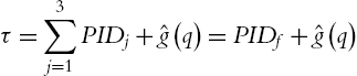
τ=3∑j=1PIDj+ˆg(q)=PIDf+ˆg(q)
Now we apply the condition (2.19) to PIDf![]() . If the gains of PIDf
. If the gains of PIDf![]() are not in the bound of (2.19), we add a new PID controller, PID4
are not in the bound of (2.19), we add a new PID controller, PID4![]() , such that the gains of PIDf+PID4
, such that the gains of PIDf+PID4![]() are in the bounds of (2.19). The final control torque to the robot is
are in the bounds of (2.19). The final control torque to the robot is
τ=PD1+PID2+PID3+PID4+ˆg(q)
Table 2.6 gives a comparative analysis of the proposed method with other PID tuning methods.
Table 2.6
Comparison of the PID tuning method
| PID tuning method | system | model | stability | systematic | adaptive |
|---|---|---|---|---|---|
| Our Method | linear/nonlinear | no | yes | yes | no |
|
Ziegler–Nichols [161] Cohen–Coon [20] |
linear | no | no | yes | no |
| Model based [24,58] | linear/nonlinear | yes | no | no | yes |
| Lyapunov method [21,22] | nonlinear | no | yes | no | no |
| Frequency domain | linear | no | no | yes | no |
| Optimization method [81] | linear | yes | no | no | no |
| Adaptive tuning [143] | linear | yes | no | no | yes |
| Intelligent method [85,129] | linear/nonlinear | no | no | no | yes |
| Impedance method [21,56] | robot | yes | no | no | no |
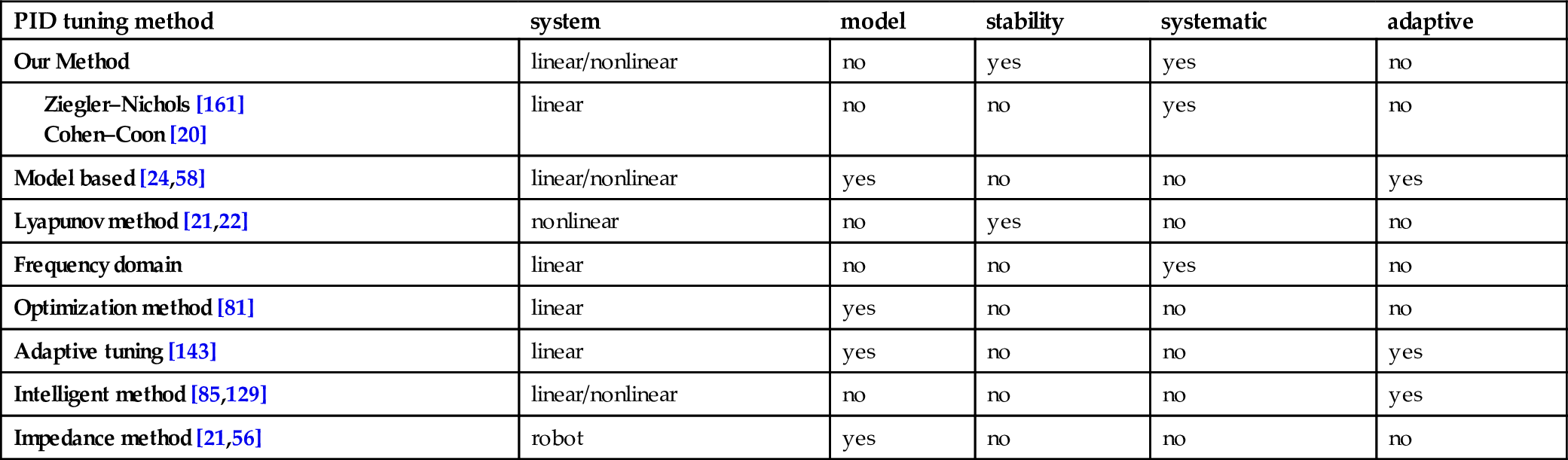
Here, we compare our method with the other eight PID tuning algorithms in six properties. It can be seen that apart from adaptive ability, our method is better than the others for robot control.
2.3 Application to an exoskeleton
The upper limb exoskeleton robot in UC-Santa Cruz is shown in Fig. 2.4. It has 7-DoF (degrees-of-freedom) as in Fig. 2.5. The computer control platform of this exoskeleton robot is a PC104 with an Intel [email protected] GHz processor and 512 Mb RAM. The motors for the first four joints are mounted in the base such that the large mass of the motors can be removed. Torque transmission from the motors to the joints is achieved using a cable system. The other three small motors are mounted in link five.
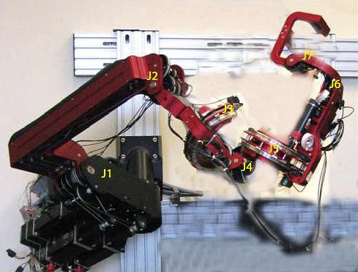

The real-time control program operated in Windows XP with Matlab 7.1, Windows Real-Time Target and C++. All of the controllers employed a sampling frequency of 1 kHz. The properties of the exoskeleton with respect to base frame are shown in Table 2.7.
Table 2.7
Parameters of the exoskeleton
| Joint | Mass (kg) | Center (m) | Length (m) |
|---|---|---|---|
| 1 | 3.4 | 0.3 | 0.7 |
| 2 | 1.7 | 0.05 | 0.1 |
| 3 | 0.7 | 0.1 | 0.2 |
| 4 | 1.2 | 0.02 | 0.05 |
| 5 | 1.8 | 0.02 | 0.05 |
| 6 | 0.2 | 0.04 | 0.1 |
| 7 | 0.5 | 0.02 | 0.05 |

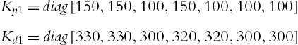
We first use the following PD1 to stabilize the robot:
Kp1=diag[150,150,100,150,100,100,100]Kd1=diag[330,330,300,320,320,300,300]
The joint velocities are estimated by the standard filters:
˜˙q(s)=bss+aq(s)=18ss+30q(s)
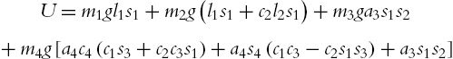
Here, the main weight of the exoskeleton is in the first four joints. The potential energy is
U=m1gl1s1+m2g(l1s1+c2l2s1)+m3ga3s1s2+m4g[a4c4(c1s3+c2c3s1)+a4s4(c1c3−c2s1s3)+a3s1s2]
The gravity compensation in (2.18) is calculated by
ˆg=∂∂qU(q)
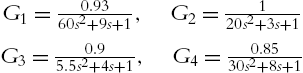
Then we use the step responses of linear systems to approximate the closed-loop responses of the robot via PD1. The step responses of the closed-loop systems of the robot and the linear systems are shown in Fig. 2.6, where in the dash lines are the step responses of the following second-order linear systems:
G1=0.9360s2+9s+1,G2=120s2+3s+1G3=0.95.5s2+4s+1,G4=0.8530s2+8s+1

In order to tuning the gains of the PID (2.29), this PID is rewritten as
PIDt=Kc(˜q+1Ti∫t0˜q(τ)dτ+Td⋅˜q)
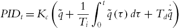
where Kc=Kp![]() is proportional gain, Ti=KcKi
is proportional gain, Ti=KcKi![]() is integral time constant, and Td=KdKc
is integral time constant, and Td=KdKc![]() is derivative time constant. We use the following tuning rule:
is derivative time constant. We use the following tuning rule:
Kc=20ξmTmKm,Ti=15ξmTm,Td=T2m10

to tune the PID parameters. This rule is similar with [58] and [24], in their case Kc=5Tm1ξmKmTm3![]() , Ti=2Tm1ξm
, Ti=2Tm1ξm![]() , Td=Tm1+0.1ξm0.8Tm1ξm
, Td=Tm1+0.1ξm0.8Tm1ξm![]() . It is different with the other two famous rules, Ziegler–Nichols and Cohen–Coon methods, where Kc=aTmKmτm
. It is different with the other two famous rules, Ziegler–Nichols and Cohen–Coon methods, where Kc=aTmKmτm![]() , Ti=2τm
, Ti=2τm![]() , Td=0.5τm
, Td=0.5τm![]() or Kc=TmKmτm(43+τm4Tm)
or Kc=TmKmτm(43+τm4Tm)![]() , Ti=τm(32Tm+6τm)13Tm+8τm
, Ti=τm(32Tm+6τm)13Tm+8τm![]() , Td=4Tmτm11Tm+2τm
, Td=4Tmτm11Tm+2τm![]() . Because their rules are suitable for the process control, our rule is for mechanical systems. By the rule (2.45) the PID2 are
. Because their rules are suitable for the process control, our rule is for mechanical systems. By the rule (2.45) the PID2 are
Kp2=diag[90,30,40,90,10,150,10]Ki2=diag[1,2,20,1.5,3,1,2]Kd2=diag[500,410,350,400,50,30,400]

The control torque becomes u=PID1+ˆg(q)+PID2![]() . The control results of Joint 1 are shown in Fig. 2.7.
. The control results of Joint 1 are shown in Fig. 2.7.
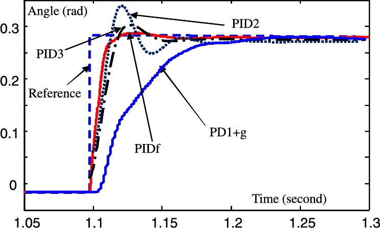
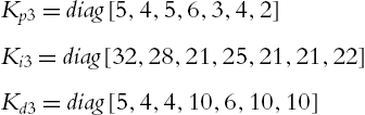
After this refine turning, PID3 is
Kp3=diag[5,4,5,6,3,4,2]Ki3=diag[32,28,21,25,21,21,22]Kd3=diag[5,4,4,10,6,10,10]
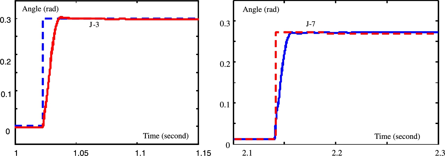
The final control is
PIDf=PD1+ˆg(q)+PID2+PID3
The stability condition (2.19) gives a sufficient condition for the minimal values of proportional and derivative gains and maximal values of integral gains. We find that the final control (2.48) satisfies the conditions (2.19). The final control results for Joint 3 and Joint 7 are shown in Fig. 2.8.
2.4 Conclusions
In this chapter the linear PID control for a class of exoskeleton robots is addressed. The conditions of the semiglobal asymptotic stability is very simple, and the linear PID control is exactly the same as the industrial controller. The systematic tuning method for PID control is proposed. This method can be applied to any robot manipulator. By using several properties of robot manipulators, the tuning process becomes simple and is easily applied in real applications. Some concepts for PID tuning are novel, such as step responses for the closed-loop systems under any PD control, and the joint torque is separated into several independent PID. We finally apply this method on an upper limb exoskeleton. Real experiment results give validation of our PID tuning method.