
PD Control with Neural Compensation
Abstract
In this chapter, we use a neural network to estimate the nonlinear terms of the exoskeleton robots, such as friction, gravity forces, and unmodeled dynamics, to guarantee stability of the closed-loop system with simple PD control law. This approach reduces the computation time with a simple neural network (NN). The learning rules obtained for the NN are very closed to the backpropagation rules [64]. This NN does not need offline previous learning, and the initial parameters are independent of the robot dynamics.
The other part of the chapter uses a modified algorithm to overcome the two drawbacks of PD control at the same time. First, the high-gain observer is joined with the normal PD control, which achieves stability with the knowledge of the friction and gravity. We use both the perturbation method and Lyapunov analysis to prove the stability, where we can see the relation between the observer error and the observer gain.
Second, we also use the RBF neural network to estimate the nonlinear terms of friction and gravity. The learning rules are obtained from the tracking error analysis. We show that the closed-loop system with high-gain observer and neural compensator is stable if the weights have certain learning rules and the observer is fast enough. Some experimental tests are carried out in order to validate the modified PD control.
Keywords
Neural networks; PD control; High-gain observer
4.1 PD control with high gain observer
The dynamics of a serial n-link rigid robot manipulator can be written as [131]
where ![]() denotes the links positions,
denotes the links positions, ![]() denotes the links velocity,
denotes the links velocity, ![]() is the inertia matrix,
is the inertia matrix, ![]() is the centripetal and Coriolis matrix,
is the centripetal and Coriolis matrix, ![]() is the gravity vector,
is the gravity vector, ![]() is a positive definite diagonal matrix of frictional terms (Coulomb friction), and
is a positive definite diagonal matrix of frictional terms (Coulomb friction), and ![]() is the input control vector.
is the input control vector.
The following properties [131] of the robot's model (4.1) are used.
Property 4.1. The centripetal and Coriolis matrix can be written as

where ![]() .
.
Property 4.2. The centripetal and Coriolis matrix satisfies the following relationship:
where ![]() .
.
Property 4.3. The centripetal and Coriolis matrix are bounded with respect to q.
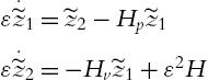
4.1.1 Singular perturbation method
A nonlinear system is said to be singularly perturbed if it has the following form:

where ![]() ,
, ![]() ,
, ![]() is a small constant parameter.
is a small constant parameter.
It is assumed that (4.2) has a unique solution with a unique equilibrium point ![]() , and has a unique root
, and has a unique root ![]() . (4.2) is in the standard form. Then it is possible to express the slow subsystem:
. (4.2) is in the standard form. Then it is possible to express the slow subsystem:
Since the second equation of (4.2) can be written as ![]() , its velocity is very fast when
, its velocity is very fast when ![]() . Let
. Let ![]() in (4.2):
in (4.2):

The fast subsystem is
where ![]() and x is treated as a fixed unknown parameter. The slow subsystem is called the quasisteady-state system and the fast subsystem is called the boundary-layer system. For singular perturbation analysis the following two assumptions should be satisfied:
and x is treated as a fixed unknown parameter. The slow subsystem is called the quasisteady-state system and the fast subsystem is called the boundary-layer system. For singular perturbation analysis the following two assumptions should be satisfied:
- 1. The equilibrium point
 of (4.5) is asymptotically stable uniformly in x and
  (the initial time).
 - 2. The eigenvalues of
 evaluated along
  of (4.3) and
  have real parts smaller than a fixed negative number, i.e.,
- where c is a positive constant.
With these assumptions, the following theorem in the Vasileva's form is established [74].
Theorem 4.1
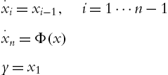
The motion equations of the serial n-link rigid robot manipulator (4.1) can be rewritten in the state space form [100]:

where ![]() is the vector of joint positions,
is the vector of joint positions, ![]() is the vector of joint velocities,
is the vector of joint velocities, ![]() is the measurable position vector.
is the measurable position vector.
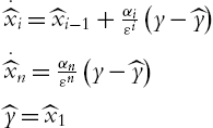
The high-gain observer has the following form [100]:

where ![]() ,
, ![]() denote the estimated values of
denote the estimated values of ![]() ,
, ![]() , respectively; ε is chosen as a small positive parameter; and
, respectively; ε is chosen as a small positive parameter; and ![]() ,
, ![]() are positive definite matrices chosen such that
are positive definite matrices chosen such that ![]() is a Hurwitz matrix. Let us define the observer error as
is a Hurwitz matrix. Let us define the observer error as
From (4.6) and (4.8) the dynamic of observer error is

If we define a new pair of variables,
(4.9) can be rewritten as

or in matrix form:
where ![]() ,
, ![]() .
.
The PD control based on a high-gain observer is
where ![]() is the desired position,
is the desired position, ![]() is the desired velocity, and
is the desired velocity, and ![]() ,
, ![]() ϵ
ϵ ![]() are constant positive matrices. We assume that the desired trajectory and its first two derivatives are bounded. The compensation terms in (4.12) are
are constant positive matrices. We assume that the desired trajectory and its first two derivatives are bounded. The compensation terms in (4.12) are ![]() .
.
The tracking errors of PD control are
From (4.6) and (4.12) the tracking errors are
or
where
Including the control (4.12) into (4.10), then
The closed-loop is the combination of (4.6), (4.12), and (4.8),

with the equilibrium point ![]() . Clearly, (4.14) has the singularly perturbed form (4.2).
. Clearly, (4.14) has the singularly perturbed form (4.2).
Let ![]() :
:
which implies that
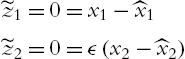
which has an equilibrium point ![]() . The system (4.14) therefore is in the standard form. Substituting the equilibrium point into the first two equations of (4.14), we obtain the quasisteady-state model:
. The system (4.14) therefore is in the standard form. Substituting the equilibrium point into the first two equations of (4.14), we obtain the quasisteady-state model:
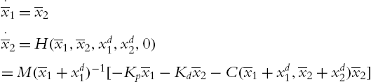
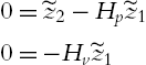
The boundary layer system of (4.14) is

where ![]() . (4.16) can be written as
. (4.16) can be written as
where ![]() and A is defined as in (4.11). The following theorem will show the stability properties of the equilibrium points
and A is defined as in (4.11). The following theorem will show the stability properties of the equilibrium points ![]() and
and ![]() for (4.15) and (4.17), respectively.
for (4.15) and (4.17), respectively.
Theorem 4.2
Proof
For the first system, consider the following candidate Lyapunov function:
with its derivative with respect to time and along (4.15),
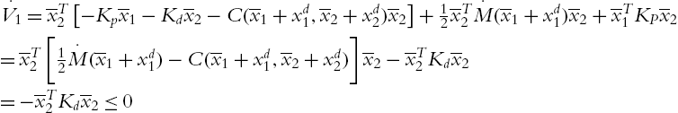
Applying LaSalle's theorem, the only solutions of (4.15) evolving in the set
are

which implies that ![]() (using Property 4.2 of the robot's dynamic).
(using Property 4.2 of the robot's dynamic).
For the second system, since A is a Hurwitz matrix, there exists a positive definite matrix P such that
where Q is a positive definite matrix.
Consider the candidate Lyapunov function:
with its derivative with respect to time and along (4.17),
□
The advantage of this approach is that the singularly perturbed analysis may divide the original problem in two systems: the slow subsystem or quasisteady state system and the fast subsystem or boundary layer system. Then both systems can be studied independently with the boundary layer system faster enough compared with the slow subsystem. These two subsystems explain why the dynamic of the high-gain observer is faster than the dynamic of the robot and the PD control. If the slow subsystem is considered as static the high-gain observer in the fast time scale τ can make the estimated states ![]() converge to the real states
converge to the real states ![]() . In the slow time scale t the slow subsystem composed by the robot and the PD control can use then the estimated states
. In the slow time scale t the slow subsystem composed by the robot and the PD control can use then the estimated states ![]() .
.
Remark 4.1
From the point of the singular perturbation analysis, one can see that the high-gain observer (4.8) has a faster dynamic than the robot (4.6) and the PD control (4.12). Under the assumption of ![]() , the observer error and the tracking error of PD control are asymptotic stable if the joint velocities are measurable.
, the observer error and the tracking error of PD control are asymptotic stable if the joint velocities are measurable.
Since it is impossible for the high-gain observer (4.8) to have ![]() , it is necessary to find a positive value of ϵ for which the stability properties are valid. For this purpose, we proposed a modified version of [120].
, it is necessary to find a positive value of ϵ for which the stability properties are valid. For this purpose, we proposed a modified version of [120].
Theorem 4.3
Proof
Let us select Lyapunov function for (4.14) as
whose derivative with respect to time and along the trajectories of (4.14),
From Theorem 4.2, we have

At this point, we need to solve

Notice that this matrix is bounded because F and ![]() are constant matrices and property 6 of the robot's dynamic.
are constant matrices and property 6 of the robot's dynamic.
Using the robot's dynamic Property 4.1 and Property 4.2 and (4.22), we can conclude that
Applying (4.22) and (4.23) to (4.21),
where 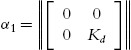 ,
, ![]() ,
,  ,
, ![]() ,
, ![]()
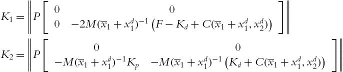
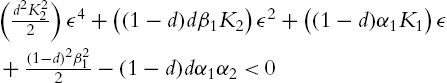
(4.24) can be written in a matrix form as

where ![]() . T has to be a positive definite matrix, and T is positive definite if there exists a continuous interval
. T has to be a positive definite matrix, and T is positive definite if there exists a continuous interval ![]() such that for all ϵ∈ Γ satisfies
such that for all ϵ∈ Γ satisfies
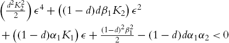
Then ![]() will be the upper bound of ϵ. □
will be the upper bound of ϵ. □
Remark 4.2
4.1.2 Lyapunov method
The motion equations of the serial n-link rigid robot manipulator (4.1) can be rewritten in the state space form (4.6). We assume u to be a bounded feedback control ![]() ,
, ![]() , so (4.6) can be rewritten as
, so (4.6) can be rewritten as
where ![]() . If the solution of (4.25) exists, for any
. If the solution of (4.25) exists, for any ![]() , it is reasonable to make following assumption.
, it is reasonable to make following assumption.
A4.1: The function ![]() is bounded over
is bounded over ![]() .
.
Let us construct the high-gain observer as
where ε is a small positive parameter and positive constant ![]() are chosen such that the roots of
are chosen such that the roots of
have negative real parts. The observer error is defined as
Theorem 4.4
Proof
The error dynamics corresponding to (4.25) and (4.26) are

If we define ![]() , the error equation (4.29) is
, the error equation (4.29) is
where 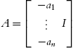 ,
, ![]() . Because
. Because ![]() satisfies (4.27), there exists a positive definite matrix P such that
satisfies (4.27), there exists a positive definite matrix P such that
Now let us define a Lyapunov function as ![]() , considering (4.30) we have
, considering (4.30) we have

Under the assumption A4.1, we may conclude that ![]() is bounded as
is bounded as
So (4.31) is
It is noted that if
then ![]() ,
, ![]() , ξ is bounded. It is easy to see that, for
, ξ is bounded. It is easy to see that, for ![]() ,
, ![]() ,
, ![]() , the condition (4.33) means
, the condition (4.33) means ![]() . As
. As ![]() , for and finite T,
, for and finite T, ![]() can be made arbitrarily small for values of
can be made arbitrarily small for values of ![]() . Furthermore, if
. Furthermore, if ![]() can be small as
can be small as ![]() ,
, ![]() , and
, and ![]() is bounded over
is bounded over ![]() (A4.1), then
(A4.1), then
So
That means ![]() , from the error equation (4.30)
, from the error equation (4.30) ![]() . Using Barlalat's lemma, we have (4.28). □
. Using Barlalat's lemma, we have (4.28). □
4.2 PD control with neural compensator
It is well known that the PD control with friction and gravity compensation may reach asymptotic stable [71]. Using neural networks to compensate the nonlinearity of the robot dynamic may be found in [85] and [78]. In [85] the authors used neural networks to approximate the whole nonlinearity of the robot dynamic. With this neural feedforward compensator and a PD control, they can guarantee a good track performance.
4.2.1 PD control with single layer neural compensation
If G and F are unknown, a neural network can be used to approximate them as
where η is bounded modeling error, ![]() ,
, ![]() is any matrix such that
is any matrix such that ![]() ,
, ![]() is the activation function, x is the input to the NN,
is the activation function, x is the input to the NN,
f is the other uncertainties.
The neural PD control is
Let us define the tracking error as
where ![]() ,
, ![]() ,
, ![]() ,
, ![]() , and the auxiliary error is defined as
, and the auxiliary error is defined as
If the Lyapunov function candidate is
and the updating law is ![]() , using
, using
So
where ![]() is upper bound of η. To guarantee stability, we need
is upper bound of η. To guarantee stability, we need ![]() . The tacking error is bounded, and
. The tacking error is bounded, and ![]() converges to
converges to ![]() .
.
Or as in [86], ![]() can be transformed into
can be transformed into
where α is a positive constant. In order to assure ![]() , we need
, we need ![]() . This means
. This means
4.2.2 PD control with a multilayer feedforward neural compensator
The friction and gravity in (4.1) can be also approximated by the multilayer neural network:
where ![]() , where
, where ![]() ,
, ![]() are fixed bounded weights,
are fixed bounded weights, ![]() is the approximated error, whose magnitude depends on the values of
is the approximated error, whose magnitude depends on the values of ![]() and
and ![]() .
.
The estimation of ![]() may be defined as
may be defined as ![]() :
:
In order to implement the neural networks, the following assumption for ![]() in (4.40) is needed:
in (4.40) is needed:
It is clear that Φ satisfies the Lipschitz condition:
where Λ is a positive definite matrix, ![]() ,
,
Remark 4.4
One can see that this condition is similar with [85] (Taylor series). The upper bound found for ![]() will be essential for proving stability of the PD control with a high gain observer and neural compensator.
will be essential for proving stability of the PD control with a high gain observer and neural compensator.
We first assume the velocities are measurable, so the PD control is
where ![]() is the desired position and
is the desired position and ![]() is the desired velocity. They are defined in (4.37). We assume the references are bounded as
is the desired velocity. They are defined in (4.37). We assume the references are bounded as
The input control vector is ![]() .
. ![]() and
and ![]() are positive defined matrices corresponding to proportional and derivative coefficients.
are positive defined matrices corresponding to proportional and derivative coefficients.
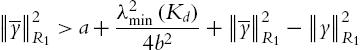
Theorem 4.5
If the following learning laws for the weights of neural networks (4.41) are used
where ![]() ,
,

then:
(I) The weights of neural networks ![]() ,
, ![]() , and tracking error
, and tracking error ![]() are bounded.
are bounded.
(II) For any ![]() the tracking error
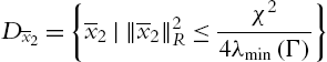
the tracking error ![]() converges to the residual set
converges to the residual set
Proof
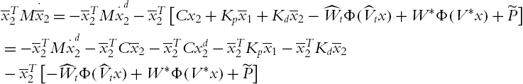
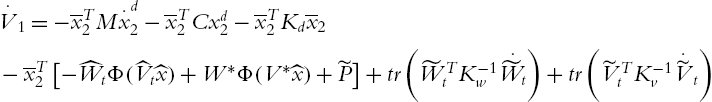
From (4.45) the closed-loop system is
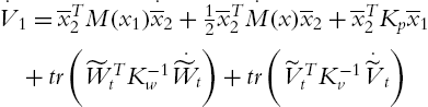
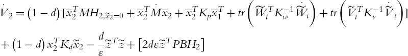
The proposed candidate Lyapunov function is
where ![]() and
and ![]() are any positive definite constant matrices. The derivative of (4.49) is
are any positive definite constant matrices. The derivative of (4.49) is
Using (4.48),
Using Property 4.2 and (4.51), (4.50) becomes
The term ![]() can be expressed as
can be expressed as
In view of the matrix inequality,
which is valid for any ![]() and for any positive defined matrix
and for any positive defined matrix ![]() [153].
[153].
![]() can be estimated as
can be estimated as

where ![]() . Using
. Using
So
where

If ![]() , using adaptive law (4.46),
, using adaptive law (4.46),
If ![]() ,
, ![]() keeps constant,
keeps constant, ![]() is bounded, that is, (I). So the total time during which
is bounded, that is, (I). So the total time during which ![]() is finite. Let
is finite. Let ![]() denote the time interval during which
denote the time interval during which ![]() :
:
- • If only finite times that
 stay outside the circle of radius
  (and then reenter), will eventually stay inside of this circle.
 - • If leave the circle infinite times, since the total time leave the circle is finite,

So ![]() is bounded via an invariant set argument. From (4.48),
is bounded via an invariant set argument. From (4.48), ![]() is also bounded. Let
is also bounded. Let ![]() denote the largest tracking error during the
denote the largest tracking error during the ![]() interval. Bounded
interval. Bounded ![]() imply that
imply that
So ![]() will convergence to
will convergence to ![]() (II) is achieved. □
(II) is achieved. □
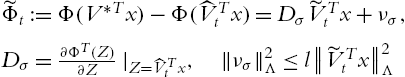
The neural networks compensation does not require structure information of the uncertainties. The RBF neural networks are more powerful [50]; we can also use RBF neural networks to approximate the friction and gravity in (4.1). The RBF neural networks is
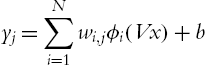
where N is a hidden nodes number, ![]() is the weight connecting the hidden layer and the output layer. x is the input vector
is the weight connecting the hidden layer and the output layer. x is the input vector ![]() (m is input node number),
(m is input node number), ![]() is the weight matrix in the hidden layer,
is the weight matrix in the hidden layer, ![]() is the radial basis function, which we select it as the Gaussian function
is the radial basis function, which we select it as the Gaussian function ![]() . Here,
. Here, ![]() and
and ![]() represent the center and spread of the basis function. b is the threshold. The significance of the threshold is that the output values have a nonzero mean. It can be combined with the first term as
represent the center and spread of the basis function. b is the threshold. The significance of the threshold is that the output values have a nonzero mean. It can be combined with the first term as ![]() ,
, ![]() , so
, so ![]() . The friction and gravity of (4.1) can be approximated by a RBF neural network (4.58) as
. The friction and gravity of (4.1) can be approximated by a RBF neural network (4.58) as
where ![]() ,
, ![]() .
. ![]() ,
, ![]() is the approximated error.
is the approximated error. ![]() and
and ![]() are unknown optimal matrices to make
are unknown optimal matrices to make ![]() minimum. The estimation of
minimum. The estimation of ![]() may be defined as
may be defined as ![]() :
:
In order to implement neural networks, Assumption A4.1 for approximation error ![]() is necessary.
is necessary.
It is clear that the Gaussian function used in RBF neural networks satisfy the Lipschitz condition. So we may conclude that
where ![]() ,
, ![]() , Λ is a positive definite matrix, l is a positive constant,
, Λ is a positive definite matrix, l is a positive constant, ![]() ,
, ![]() .
.
The learning rules of ![]() and
and ![]() are derived from the stability analysis of the closed-loop system when the neural compensator (4.60) is combined with normal PD control as
are derived from the stability analysis of the closed-loop system when the neural compensator (4.60) is combined with normal PD control as
where ![]() and
and ![]() are positive defined matrices corresponding to proportional and derivative coefficients,
are positive defined matrices corresponding to proportional and derivative coefficients, ![]() is the desired position.
is the desired position. ![]() is the desired velocity.
is the desired velocity.
Remark 4.5
From the definition of the Lyapunov function (4.49), we may see that the learning rules (4.46) will minimize the tracking error ![]() . This structure is different from normal neural networks which are used for approximation of nonlinear function. The first terms
. This structure is different from normal neural networks which are used for approximation of nonlinear function. The first terms ![]() and
and ![]() are exactly corresponding to the backpropagation scheme. The second terms
are exactly corresponding to the backpropagation scheme. The second terms ![]() and
and ![]() are additional ones, which can assure a stable learning. Deriving an update law with guaranteed stability is a very effective technique; some similar analysis may be found in [85].
are additional ones, which can assure a stable learning. Deriving an update law with guaranteed stability is a very effective technique; some similar analysis may be found in [85].
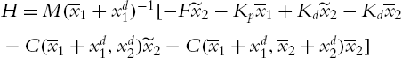
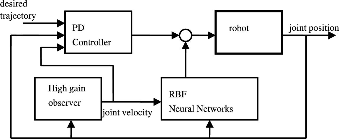
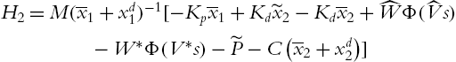
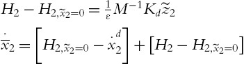
4.3 PD control with velocity estimation and neural compensator
If neither the velocity ![]() nor the friction and gravity are known, the normal PD control should be combined with velocities estimation and neural compensations:
nor the friction and gravity are known, the normal PD control should be combined with velocities estimation and neural compensations:
where ![]() . The structure of the new PD controller is shown in Fig. 4.1.
. The structure of the new PD controller is shown in Fig. 4.1.
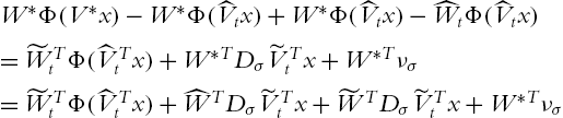
The dynamic of the tracking error can be formed from (4.6) and (4.63)
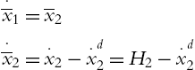
where
The closed-loop system is

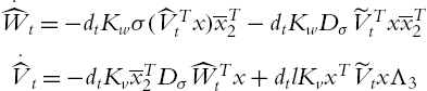
The new updating law, which is obtained from next theorem is

where ![]() ,
,
![]() ,
, ![]() ,
, ![]() . We can see that another condition is needed: M is known. This requirement is necessary if both velocity and friction are unknown (see [78]). When we realize the high-gain observer (4.8), we can see that the observer error is less than
. We can see that another condition is needed: M is known. This requirement is necessary if both velocity and friction are unknown (see [78]). When we realize the high-gain observer (4.8), we can see that the observer error is less than ![]() . Can we find the largest value of ε, which can assure that the closed-loop system is stable? The following theorem gives the answer to this question.
. Can we find the largest value of ε, which can assure that the closed-loop system is stable? The following theorem gives the answer to this question.
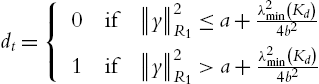
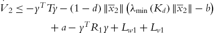
Theorem 4.6
If (a) the learning laws for the weights of neural networks (4.60) are used as in (4.67), (b) the gain of the observer satisfies
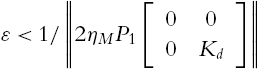
![]() is the solution of the following Lyapunov equation:
is the solution of the following Lyapunov equation:
then we have:
(I) The weights of neural networks ![]() ,
, ![]() , observer and tracking errors
, observer and tracking errors ![]() and
and ![]() are bounded.
are bounded.
(II) For any ![]() the tracking and observer error
the tracking and observer error ![]() converges to the residual set
converges to the residual set
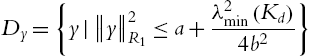
where a and b are defined in (4.68). ![]() is a positive defined matrix such that
is a positive defined matrix such that ![]() ,
, ![]() are positive constants.
are positive constants.
Proof
Let us select the following candidate Lyapunov function for (4.66):
where ![]() ,
, ![]() is the Lyapunov function in Theorem 4.4 as in (4.49). Since PD control (4.63) is different from (4.62), we cannot apply
is the Lyapunov function in Theorem 4.4 as in (4.49). Since PD control (4.63) is different from (4.62), we cannot apply ![]() in Theorem 4.5. From (4.66), we know
in Theorem 4.5. From (4.66), we know ![]() . Because
. Because
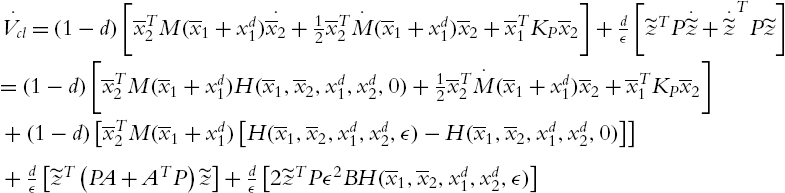
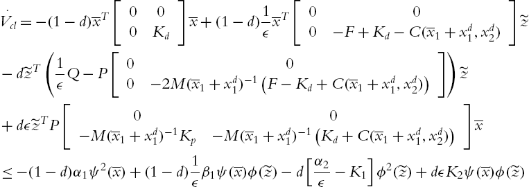
the derivative of (4.71) is
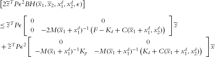
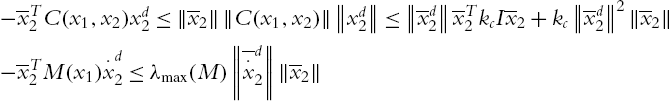
Compare (4.72) and (4.48) and the first term of right-hand side is the same as (4.50):
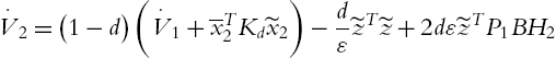
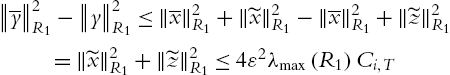
From (4.65),

![]() can be estimated as
can be estimated as

![]() may be estimated as
may be estimated as
![]() becomes
becomes
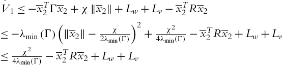
So
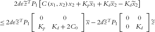
(4.73) becomes
We want to make T as a positive defined matrix, i.e.,
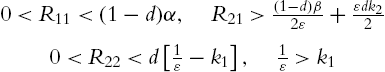
Since ![]() ,
, ![]() can be any positive constant. So if condition (4.69) is satisfied,
can be any positive constant. So if condition (4.69) is satisfied, ![]() is selected as (4.77),
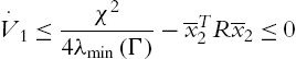
is selected as (4.77), ![]() . So
. So

where (4.78) has a same structure as in Theorem 4.4, with the similar proof (I) and (II) may be established. □
Remark 4.6
Since ![]() is not measurable, the dead zone
is not measurable, the dead zone ![]() in (4.68) cannot be realized. We will use the available date
in (4.68) cannot be realized. We will use the available date ![]() to determine the dead zone. The dead zone can be represented as
to determine the dead zone. The dead zone can be represented as
Because ![]() ,
,
So, the new dead zone is modified as

4.4 Simulation
To develop the simulations, a two-link planar robot manipulator is considered. It is assumed that each link has its mass concentrated as a point at the end. The manipulator is in vertical position, with gravity and friction. The robot parameters are: ![]() ,
, ![]() ,
, ![]() . The two friction coefficients are 0.3, and the gravity is 9.8. So the real matrices of (4.1) are
. The two friction coefficients are 0.3, and the gravity is 9.8. So the real matrices of (4.1) are
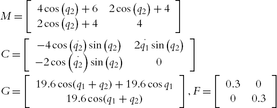
where ![]() . All data are given with the appropriate unities.
. All data are given with the appropriate unities.
The following PD coefficients are chosen:

The matrices P and Q are selected as

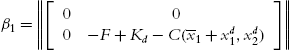
Let us calculate the constants in Theorem 4.5,  ,
, ![]() ,
,
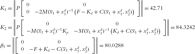
where ![]() denotes the absolute value of the real part of the maximum eigenvalue of the matrix A. Then (4.19) becomes
denotes the absolute value of the real part of the maximum eigenvalue of the matrix A. Then (4.19) becomes
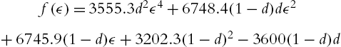
With ![]() the polynomial (4.79) is shown in Fig. 4.2.
the polynomial (4.79) is shown in Fig. 4.2.
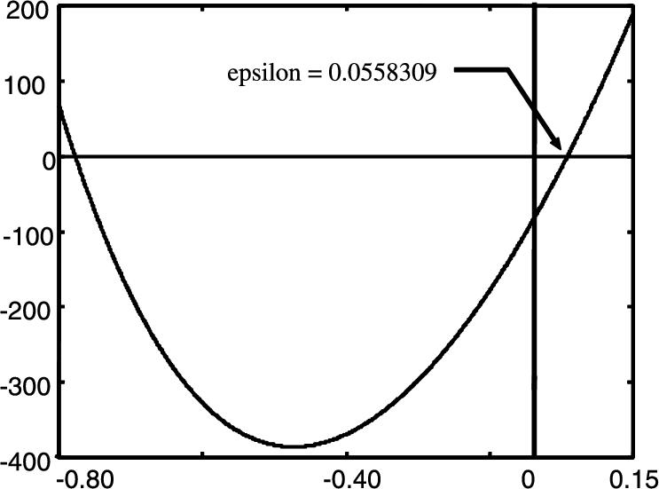
One can see that for ![]() (4.79) is negative. So
(4.79) is negative. So ![]() , i.e.,
, i.e., ![]() . The high-gain observer (4.8) is determined as
. The high-gain observer (4.8) is determined as ![]() .
.
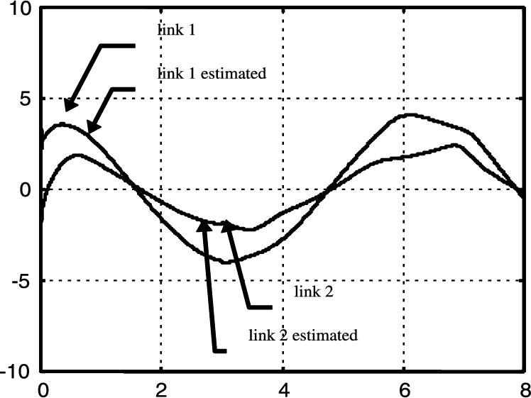
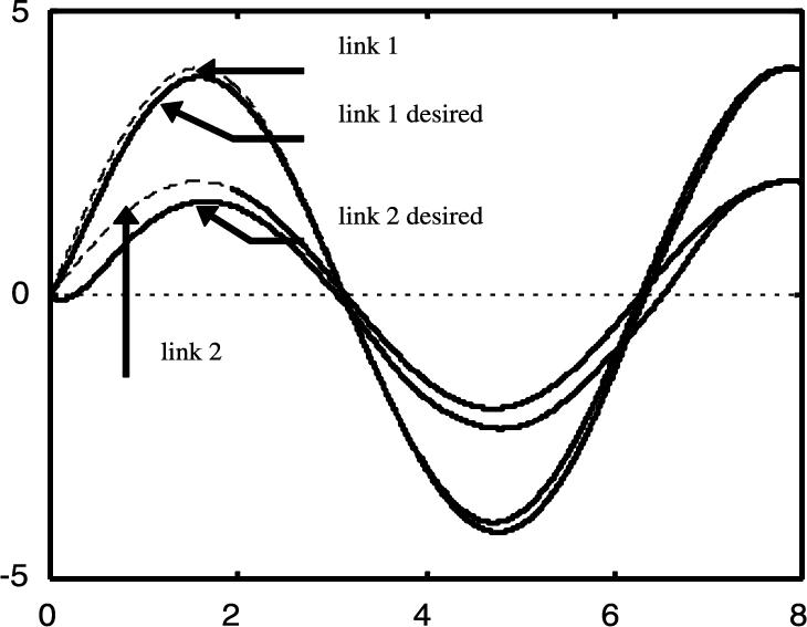
Fig. 4.3 and Fig. 4.4 show rapid convergence of the observer to the link's velocities. The observer error is almost zero in this short interval. Fig. 4.3 shows that with a velocity observer (high-gain observer), PD control can make the links follow the desired trajectory.


The asymptotic stability assures that the desired positions may be reached with zero error if ![]() . Rapid and accurate convergence of the observer is essential for the PD controller, because the observer is in the feedback loop. Since the high-gain observer (4.26) has these properties, we can use a simple controller (4.12) to compensate the uncertainties of the observer response.
. Rapid and accurate convergence of the observer is essential for the PD controller, because the observer is in the feedback loop. Since the high-gain observer (4.26) has these properties, we can use a simple controller (4.12) to compensate the uncertainties of the observer response.
Fig. 4.5 and Fig. 4.6 show the simulation results of the performance of the high-gain observer when a noise arises at ![]() . The perturbation is a
. The perturbation is a ![]() increment on the second link's mass. This is intended to see the robustness of the observer-based PD control. Fig. 4.7 shows the tracking done by both links of the robot with the same perturbation at
increment on the second link's mass. This is intended to see the robustness of the observer-based PD control. Fig. 4.7 shows the tracking done by both links of the robot with the same perturbation at ![]() .
.
Since the observer and controller are independent of the robot's dynamics, the influence of perturbations are very small. All data are given with the appropriate unities. The following PD coefficients are chosen:

Friction and gravity can be uniformly approximated by a radial basis function as in (4.60) with ![]() . The Gaussian function is
. The Gaussian function is

where the spread ![]() was set to
was set to ![]() and the center
and the center ![]() is a random number between 0 and 1. The control law applied is
is a random number between 0 and 1. The control law applied is
starting with ![]() and
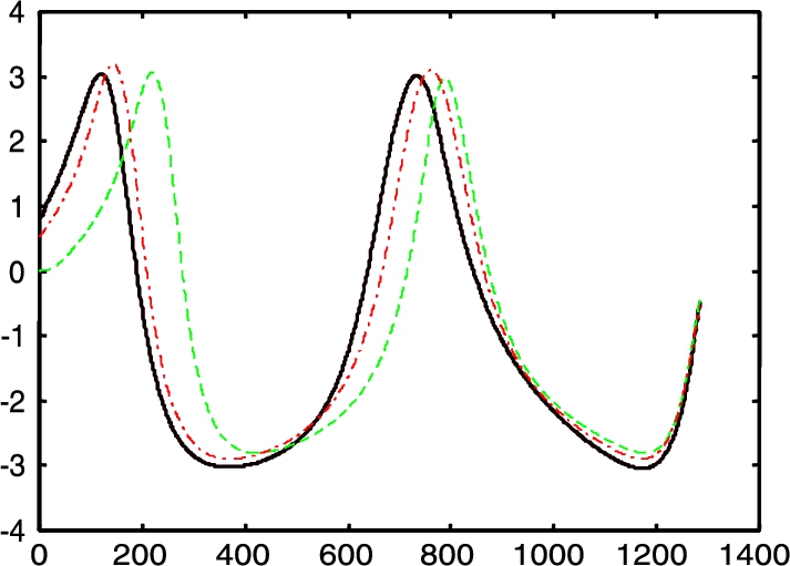
and ![]() as initial values. Even though some initial weights are needed for the controller to work, no special values are required nor is a previous investigation on the robot dynamics for the implementation of this control. Fig. 4.7 and Fig. 4.8 gave the comparison of the performance of PD controller neural compensation. The continuous line is the exact position, the dashed line is general PD control without friction and gravity, and the dashed-dotted line is the neural networks compensation.
as initial values. Even though some initial weights are needed for the controller to work, no special values are required nor is a previous investigation on the robot dynamics for the implementation of this control. Fig. 4.7 and Fig. 4.8 gave the comparison of the performance of PD controller neural compensation. The continuous line is the exact position, the dashed line is general PD control without friction and gravity, and the dashed-dotted line is the neural networks compensation.
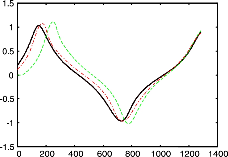
We can see that PD control with the RBF networks compensator may improve the control performance.
4.5 Conclusions
The disadvantages of the popular PD control are overcome in the following two ways: (I) A high-gain observer is proposed for the estimation of the velocities of the joints. (II) The RBF neural networks are used to compensate the gravity and friction. By the singular perturbation and Lyapunov-like analysis, we give proofs of the high-gain observer and the stability of the closed-loop system with the velocity estimation and the RBF compensator.