
PID Control with Neural Compensation
Abstract
The simplest method to decrease the tracking error of PD control is to add an integral action, i.e., change the neural PD control into neural PID control. A natural question is: Why do we not add an integrator instead of increasing derivative gain in the neural PD control?
In this chapter, the well-known neural PD control of robot manipulators is extended to the neural PID control. It is an industrial linear PID controller adding a neural compensator. The semiglobal asymptotic stability of this novel neural control is proven. Explicit conditions for choosing PID gains are given. When the measurement of velocities it is not available, local asymptotic stability is also proven with a velocity observer. Unlike the other neural controllers of robot manipulators, our neural PID does not need a big derivative and integral gains to assure asymptotic stability. We apply this neural control to our 3-DoF exoskeleton robot in CINVESTA-IPN. Experimental results show that this neural PID control has many advantages over classic PID control, neural PD control, and the other neural PID control.
Keywords
Neural networks; Linear PID control
5.1 Stable neural PID control
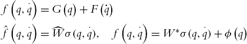
Without flexible links and high-frequency joint dynamics, rigid robots can be expressed in the Lagrangian form:
where ![]() represents the link positions.
represents the link positions. ![]() is the inertia matrix,
is the inertia matrix, ![]() represents centrifugal force,
represents centrifugal force, ![]() is a vector of gravity torques, and
is a vector of gravity torques, and ![]() is friction. All terms
is friction. All terms ![]() ,
, ![]() ,
, ![]() , and
, and ![]() are unknown.
are unknown. ![]() is the control input. The friction
is the control input. The friction ![]() is represented by the Coulomb friction model:
is represented by the Coulomb friction model:
where ![]() is a large positive constant, such that
is a large positive constant, such that ![]() can approximate
can approximate ![]() , and
, and ![]() and
and ![]() are positive coefficients. In this paper, we use a simple model for the friction as in [85] and [71],
are positive coefficients. In this paper, we use a simple model for the friction as in [85] and [71],
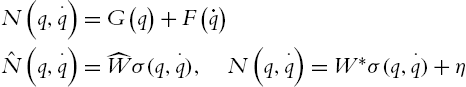
When ![]() and
and ![]() are unknown, we may use a neural network to approximate them as
are unknown, we may use a neural network to approximate them as
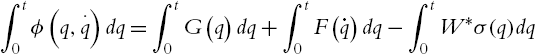
where ![]() is an unknown constant weight,
is an unknown constant weight, ![]() is the estimated weight,
is the estimated weight, ![]() is the neural approximation error, σ is a neural activation function. Here, we use the Gaussian function such that
is the neural approximation error, σ is a neural activation function. Here, we use the Gaussian function such that ![]() .
.
Since the joint velocity ![]() is not always available, we may use a velocity observer to approximate it. This linear-in-the-parameter net is the simplest neural network. According to the universal function approximation theory, the smooth function
is not always available, we may use a velocity observer to approximate it. This linear-in-the-parameter net is the simplest neural network. According to the universal function approximation theory, the smooth function ![]() can be approximated by a multilayer neural network with one hidden layer in any desired accuracy provided proper weights and hidden neurons:
can be approximated by a multilayer neural network with one hidden layer in any desired accuracy provided proper weights and hidden neurons:
where ![]() ,
, ![]() , m is hidden node number,
, m is hidden node number, ![]() is the weight in the hidden layer. In order to simplify the theory analysis, we first use linear-in-the-parameter net (5.4). Then we will show that the multilayer neural network (5.5) can also be used for the neural control of robot manipulators. The robot dynamics (5.1) have the following standard properties [131], which will be used to prove stability.
is the weight in the hidden layer. In order to simplify the theory analysis, we first use linear-in-the-parameter net (5.4). Then we will show that the multilayer neural network (5.5) can also be used for the neural control of robot manipulators. The robot dynamics (5.1) have the following standard properties [131], which will be used to prove stability.
P5.1. The inertia matrix ![]() is symmetric positive definite, and
is symmetric positive definite, and
where ![]() and
and ![]() are the maximum and minimum eigenvalues of the matrix M.
are the maximum and minimum eigenvalues of the matrix M.
P5.2. For the centrifugal and Coriolis matrix ![]() , there exists a number
, there exists a number ![]() such that
such that
and ![]() is skew symmetric, i.e.,
is skew symmetric, i.e.,
also
P5.3. The neural approximation error ![]() is Lipschitz over q and
is Lipschitz over q and ![]()
From (5.4), we know
Because ![]() and
and ![]() satisfy the Lipschitz condition, P5.3 is established.
satisfy the Lipschitz condition, P5.3 is established.
In order to simplify calculation, we use the simple model for the friction as in (5.3). The lower bound of ![]() can be estimated as
can be estimated as
where ![]() is the potential energy of the robot,
is the potential energy of the robot, ![]() . Since
. Since ![]() is a Gaussian function,
is a Gaussian function, ![]() . By
. By ![]() ,
,
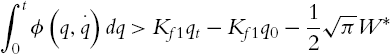
where ![]() . Since the work space of a manipulator (the entire set of points reachable by the manipulator) is known,
. Since the work space of a manipulator (the entire set of points reachable by the manipulator) is known, ![]() can be estimated. We define the lower bound of
can be estimated. We define the lower bound of ![]() as
as
Given a desired constant position ![]() , the objective of robot control is to design the input torque u in (5.1) such that the regulation error
, the objective of robot control is to design the input torque u in (5.1) such that the regulation error
![]() and
and ![]() when initial conditions are in arbitrary large domain of attraction.
when initial conditions are in arbitrary large domain of attraction.
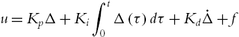
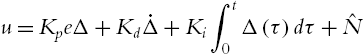
The classic industrial PID law is
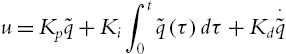
where ![]() ,
, ![]() , and
, and ![]() are proportional, integral, and derivative gains of the PID controller, respectively.
are proportional, integral, and derivative gains of the PID controller, respectively.
When the unknown dynamic ![]() in (5.4) is big, in order to assure asymptotic stability, the integral gain
in (5.4) is big, in order to assure asymptotic stability, the integral gain ![]() has to be increased. This may cause big overshoot, bad stability, and integrator windup. Model-free compensation is an alternative solution, where
has to be increased. This may cause big overshoot, bad stability, and integrator windup. Model-free compensation is an alternative solution, where ![]() is estimated by a neural network as in (5.4). Normal neural PD control is [85]
is estimated by a neural network as in (5.4). Normal neural PD control is [85]
where ![]() . With the filtered error
. With the filtered error ![]() , (5.16) becomes
, (5.16) becomes
The control (5.17) avoids integrator problems in (5.15). Unlike industrial PID control, they cannot reach asymptotic stability. The stability condition of the neural PD control (5.16) is ![]() , B is a constant [87]. In order to decrease
, B is a constant [87]. In order to decrease ![]() ,
, ![]() has to be increased. This causes a long settling time problem. The asymptotic stability (
has to be increased. This causes a long settling time problem. The asymptotic stability (![]() ) requires
) requires ![]() .
.
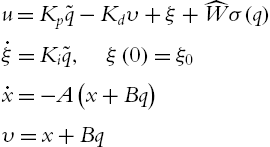
An integrator is added into the normal neural PD control (5.16). It has a similar form as the industrial PID in (5.15),

Because in the regulation case ![]() ,
, ![]() , the PID control law can be expressed via the following equations:
, the PID control law can be expressed via the following equations:

We require the PID control part of (5.19) is decoupled, i.e., ![]() , and
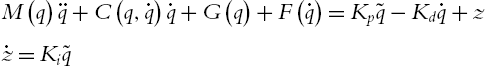
, and ![]() are positive definite diagonal matrices. The closed-loop system of the robot (5.1) is
are positive definite diagonal matrices. The closed-loop system of the robot (5.1) is

where ![]()
Here, ![]() . In matrix form the closed-loop system is
. In matrix form the closed-loop system is
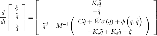
The equilibrium of (5.22) is ![]() . Since at equilibrium point
. Since at equilibrium point ![]() and
and ![]() the equilibrium is
the equilibrium is ![]() . We simplify
. We simplify ![]() as
as ![]() .
.
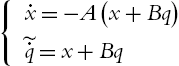
In order to move the equilibrium to the origin, we define
The final closed-loop equation becomes
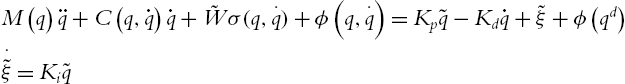
The following theorem gives the stability analysis of the neural PID control. From this theorem, we can see how to choose the PID gains and how to train the weight of the neural compensator in (5.19). Another important conclusion is that the neural PID control (5.19) can force the error ![]() to zero.
to zero.
Theorem 5.1
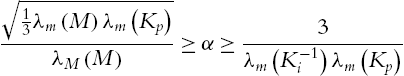
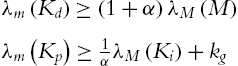
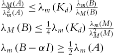
Consider the robot dynamic (5.1) controlled by the neural PID control (5.19). The closed-loop system (5.24) is semiglobally asymptotically stable at the equilibrium ![]() , provided that control gains satisfy
, provided that control gains satisfy

where ![]() ,
, ![]() satisfies (5.10), and the weight of the neural networks (5.4) is tuned by
satisfies (5.10), and the weight of the neural networks (5.4) is tuned by
where α is positive design constant, it satisfies
Proof
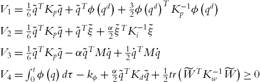
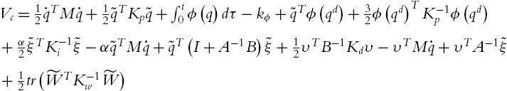
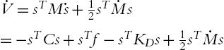
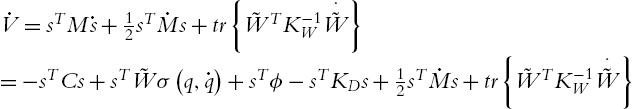
We construct a Lyapunov function as
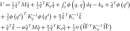
where ![]() is defined in (5.13) such that
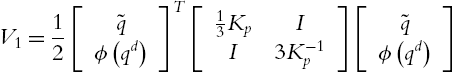
is defined in (5.13) such that ![]() . α is a design positive constant. We first prove V is a Lyapunov function,
. α is a design positive constant. We first prove V is a Lyapunov function, ![]() . The term
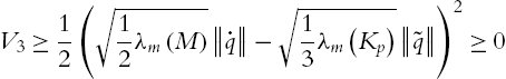
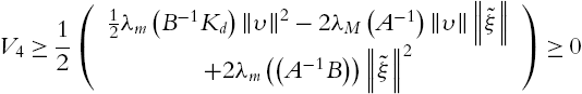
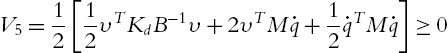
. The term ![]() is separated into three parts, and
is separated into three parts, and ![]() :
:
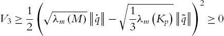
It is easy to find
Since ![]() ,
, ![]() is a semipositive definite matrix,
is a semipositive definite matrix, ![]() . When
. When ![]() ,
,

Because
when ![]() ,
,
Obviously, if

there exists
This means if ![]() is sufficiently large or
is sufficiently large or ![]() is sufficiently small, (5.34) is established, and
is sufficiently small, (5.34) is established, and ![]() is globally positive definite. Using
is globally positive definite. Using ![]() ,
, ![]() and
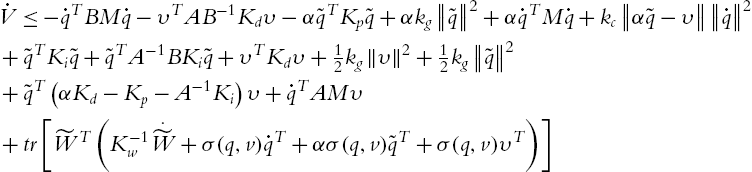
and ![]() , the derivative of V is
, the derivative of V is
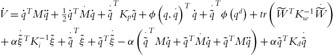
Using (5.8) the first three terms of (5.36) become
And
If
and
then ![]() ,
, ![]() decreases. Then (5.40) is established. Using (5.34) and
decreases. Then (5.40) is established. Using (5.34) and ![]() , (5.40) is (5.25).
, (5.40) is (5.25).
![]() is negative semidefinite. Define a ball Σ of radius
is negative semidefinite. Define a ball Σ of radius ![]() centered at the origin of the state space, which satisfies these conditions:
centered at the origin of the state space, which satisfies these conditions:
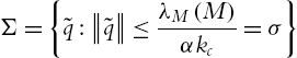
![]() is negative semidefinite on the ball Σ. There exists a ball Σ of radius
is negative semidefinite on the ball Σ. There exists a ball Σ of radius ![]() centered at the origin of the state space on which
centered at the origin of the state space on which ![]() . The origin of the closed-loop equation (5.24) is a stable equilibrium. Since the closed-loop equation is autonomous, we use LaSalle's theorem. Define Ω as
. The origin of the closed-loop equation (5.24) is a stable equilibrium. Since the closed-loop equation is autonomous, we use LaSalle's theorem. Define Ω as

From (5.36), ![]() if and only if
if and only if ![]() . For a solution
. For a solution ![]() to belong to Ω for all
to belong to Ω for all ![]() , it is necessary and sufficient that
, it is necessary and sufficient that ![]() for all
for all ![]() . Therefore it must also hold that
. Therefore it must also hold that ![]() for all
for all ![]() . We conclude from the closed-loop system (5.24) that if
. We conclude from the closed-loop system (5.24) that if ![]() for all
for all ![]() , then
, then
implies that ![]() for all
for all ![]() . So
. So ![]() is the only initial condition in Ω for which
is the only initial condition in Ω for which ![]() for all
for all ![]() .
.
Finally, we conclude from all of this that the origin of the closed-loop system (5.24) is locally asymptotically stable. Because ![]() , the upper bound for
, the upper bound for ![]() can be
can be
It establishes the semiglobal stability of our controller, in the sense that the domain of attraction can be arbitrarily enlarged with a suitable choice of the gains. Namely, increasing ![]() the basin of attraction will grow. □
the basin of attraction will grow. □
Remark 5.1
From the above stability analysis, we see that the gain matrices of the neural PID control (5.19) can be chosen directly from the conditions (5.25). The tuning procedure of the PID parameters is more simple than [2,4,71,101,117]. No modeling information is needed. The upper or lower bounds of PID gains need the maximum eigenvalue of M in (5.25); it can be estimated without calculating M. For a robot with only revolute joints [131],

where ![]() stands the ijth element of M,
stands the ijth element of M, ![]() . A β can be selected such that it is much bigger than all elements.
. A β can be selected such that it is much bigger than all elements.
Remark 5.2
The main difference between our neural PID control with the other neural PD controllers is that the stability condition is changed. We require the regulation error:
The other neural PD controllers need

where ![]() and
and ![]() are positive constants. Obviously, if the initial condition is not worse and satisfies (5.46), (5.46) is always satisfied, and
are positive constants. Obviously, if the initial condition is not worse and satisfies (5.46), (5.46) is always satisfied, and ![]() will decrease to zero. But (5.47) cannot be satisfied when
will decrease to zero. But (5.47) cannot be satisfied when ![]() becomes small, so
becomes small, so ![]() has to be increased.
has to be increased.
Remark 5.3
If the unknown ![]() is estimated by the multilayer neural network (5.5) the modeling error (5.21) becomes
is estimated by the multilayer neural network (5.5) the modeling error (5.21) becomes

where ![]() ,
, ![]() is the Taylor approximation error. The closed-loop equation (5.24) becomes
is the Taylor approximation error. The closed-loop equation (5.24) becomes

If the Lyapunov function in (5.28) is changed as
then the derivative of (5.50) is

If the training rule (5.26) is changed as

Theorem 5.1 is also established.
One common problem of the linear PID control (5.18) is integral windup, where the rate of integration is larger than the actual speed of the system. The integrator's output may exceed the saturation limit of the actuator. The actuator will then operate at its limit no matter what the process outputs. This means that the system runs with an open loop instead of a constant feedback loop. The solutions of antiwindup schemes are mainly classified into two types [142]: conditional integration and back-calculation. It has been shown that none of the existed methods is able to provide good performance over a wide range of processes [5]. In this paper, we use the conditional integration algorithm. The integral term is limited to a selected value
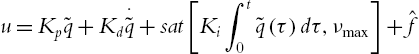
where ![]() .
. ![]() is a prescribed value to the integral term when the controller saturates. This approach is also called preloading [123]. Now the linear PID controller becomes nonlinear PID. The semiglobal asymptotic stability has been analyzed by [2]. When
is a prescribed value to the integral term when the controller saturates. This approach is also called preloading [123]. Now the linear PID controller becomes nonlinear PID. The semiglobal asymptotic stability has been analyzed by [2]. When ![]() is the maximum torque of all joint actuators,
is the maximum torque of all joint actuators, ![]() ,
, ![]() ,
, ![]() . A necessary condition is
. A necessary condition is
where ![]() is the gravity torque of the robot (5.1),
is the gravity torque of the robot (5.1), ![]() is the upper bound of
is the upper bound of ![]() .
. ![]() is a design factor in the case that not all PID terms are subjected to saturation. For the controller (5.53),
is a design factor in the case that not all PID terms are subjected to saturation. For the controller (5.53), ![]() can selected as
can selected as ![]() .
.
Following the process from (5.4) to (5.13), the neural PID with an antiwindup controller (5.53) requires
where ![]() is the upper bound of the neural estimator,
is the upper bound of the neural estimator, ![]() ,
, ![]() and
and ![]() are defined in (5.4).
are defined in (5.4).
We can see that the first additional condition for the neural PID with antiwindup is that the neural estimator must be bounded, while the linear neural PID only requires that the neural estimation error satisfy the Lipschitz condition (5.10).
Since ![]() (or
(or ![]() ) is a physical requirement for the actuator, it is not a design parameter. In order to satisfy the condition (5.54), we should force
) is a physical requirement for the actuator, it is not a design parameter. In order to satisfy the condition (5.54), we should force ![]() as small as possible. A good structure of the neural estimator may make the term
as small as possible. A good structure of the neural estimator may make the term ![]() smaller, such as the multilayer neural network in Remark 5.3. There are several methods that can be used to find a good neural network, such as the genetic algorithm [7] and pruning [130]. Besides structure optimization, the initial condition for the gradient training algorithm (5.26) also affects
smaller, such as the multilayer neural network in Remark 5.3. There are several methods that can be used to find a good neural network, such as the genetic algorithm [7] and pruning [130]. Besides structure optimization, the initial condition for the gradient training algorithm (5.26) also affects ![]() . Since the initial conditions for
. Since the initial conditions for ![]() and
and ![]() in (5.52) do not affect the stability property, we design an off-line method to find a better value for
in (5.52) do not affect the stability property, we design an off-line method to find a better value for ![]() and
and ![]() . If we let
. If we let ![]() ,
, ![]() , the algorithm (5.52) can make the identification error convergent, i.e.,
, the algorithm (5.52) can make the identification error convergent, i.e., ![]() and
and ![]() will make the identification error smaller than that of
will make the identification error smaller than that of ![]() and
and ![]() .
. ![]() and
and ![]() are selected by the following steps:
are selected by the following steps:
- 1. Start from any initial value for
 ,
,  .
. - 2. Do training with (5.52) until
 .
. - 3. If the
 , let
, let  and
and  as a new
  and
and  , i.e.,
  ,
,  , go to 2 to repeat the training process.
 - 4. If the
 , stop this off-line identification, now and are the final value for and
  .
.
5.2 Neural PID control with unmeasurable velocities
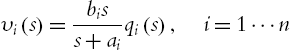
The neural PID control (5.19) uses the joint velocities ![]() . In contrast to the high precision of the position measurements by the optical encoders, the measurement of velocities by tachometers may be quite mediocre in accuracy, specifically for certain intervals of velocity. The common idea in the design of PID controllers, which requires velocity measurements, has been to propose state observers to estimate the velocity. The simplest observer may be the first-order and zero-relative position filter [131]
. In contrast to the high precision of the position measurements by the optical encoders, the measurement of velocities by tachometers may be quite mediocre in accuracy, specifically for certain intervals of velocity. The common idea in the design of PID controllers, which requires velocity measurements, has been to propose state observers to estimate the velocity. The simplest observer may be the first-order and zero-relative position filter [131]
where ![]() is an estimation of
is an estimation of ![]() ,
, ![]() , and
, and ![]() are the elements of diagonal matrices A and B,
are the elements of diagonal matrices A and B, ![]() ,
, ![]() ,
, ![]() ,
, ![]() . The transfer function (5.55) can be realized by
. The transfer function (5.55) can be realized by
The linear PID control (5.19) becomes
where ![]() ,
, ![]() , and
, and ![]() are positive definite diagonal matrices,
are positive definite diagonal matrices, ![]() and
and ![]() in (5.55) are positive constants. The closed-loop system of the robot (5.1) is
in (5.55) are positive constants. The closed-loop system of the robot (5.1) is

The equilibrium of (5.58) is ![]() .
.
The following theorem gives the asymptotic stability of the neural PID control with the velocity observer (5.55). This theorem also provides a training algorithm for neural weights, and an explicit selection method of PID gains.
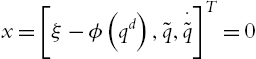
Since the velocities are not available, the input of the neural networks becomes
Theorem 5.2
Consider the robot dynamic (5.1) controlled by the neural PID controller (5.57), if A and B of the velocity observer (5.55) satisfy
where α is positive design constant, provided that the PID control gains of (5.57) satisfy
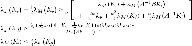
where ![]() satisfies (5.10),
satisfies (5.10), ![]() is the condition number of M, and the weight of neural networks is tuned by
is the condition number of M, and the weight of neural networks is tuned by
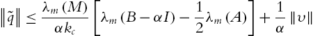
then the closed-loop system (5.58) is locally asymptotically stable at the equilibrium:
in the domain of attraction
Proof
We construct a Lyapunov function as
where the definition of ![]() is the same as Theorem 5.1. α is a design positive constant. We first prove V is a Lyapunov function,
is the same as Theorem 5.1. α is a design positive constant. We first prove V is a Lyapunov function, ![]() . The term
. The term ![]() is separated into three parts, and
is separated into three parts, and ![]() :
:

Here, ![]() and
and ![]() are the same as (5.29), i.e.,
are the same as (5.29), i.e.,
For ![]() , if
, if ![]()
Because ![]() and
and ![]() , it is easy to find that, if
, it is easy to find that, if ![]() or
or ![]() ,
,
If ![]() or
or ![]()
Because ![]() , obviously, there exist α, A, and B such that
, obviously, there exist α, A, and B such that

This means if ![]() is sufficiently large or
is sufficiently large or ![]() is sufficiently small, (5.34) is established, and
is sufficiently small, (5.34) is established, and ![]() is globally positive definite. Now we compute its derivative. The derivative of
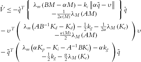
is globally positive definite. Now we compute its derivative. The derivative of ![]() is
is
Because ![]() and
and ![]() , the last term is zero if we apply the updating law (5.62). Using (5.32), (5.72) is
, the last term is zero if we apply the updating law (5.62). Using (5.32), (5.72) is
Using ![]() , i can be “m” or “M,” the last condition of (5.71) can be replaced by
, i can be “m” or “M,” the last condition of (5.71) can be replaced by
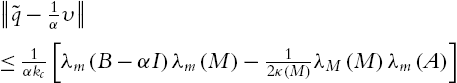
It is the attraction area (5.64).
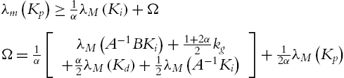
Using ![]() , the second condition of (5.71) is
, the second condition of (5.71) is

It is the condition for ![]() in (5.61). Also
in (5.61). Also
It is the condition for ![]() in (5.61). The condition for
in (5.61). The condition for ![]() in (5.61) is obtained from (5.67). The remaining part of the proof is the same as Theorem 5.1. □
in (5.61) is obtained from (5.67). The remaining part of the proof is the same as Theorem 5.1. □
Remark 5.4
The conditions (5.60) and (5.61) decide how to choose the PID gains. The first condition of (5.61) is
the third conditions of (5.61) is ![]() ; they are compatible. When
; they are compatible. When ![]() is not big, these conditions can be established. The second condition of (5.61) and the third condition of (5.60) are not directly compatible. We first let α as small as possible, and
is not big, these conditions can be established. The second condition of (5.61) and the third condition of (5.60) are not directly compatible. We first let α as small as possible, and ![]() as big as possible. So
as big as possible. So ![]() cannot be big. These requirements are reasonable for our real control. If we select
cannot be big. These requirements are reasonable for our real control. If we select ![]() , form the third condition of (5.60),
, form the third condition of (5.60), ![]() . The second condition of (5.61) requires
. The second condition of (5.61) requires ![]() , there exists
, there exists ![]() and a small α such that
and a small α such that ![]() . After A and B are decided, we use the second condition of (5.61) to select
. After A and B are decided, we use the second condition of (5.61) to select ![]() .
.
5.3 Neural PID tracking control
We modify the reference signal and add a filter, such that the PID regulation control is extended to PID tracking control. Most important, the global and semiglobal asymptotic stability of this PID tracking control are proved.
Model-based compensation is an alternative method for PID control to overcome the problems of PID control. The intelligent compensation does not need a mathematical model; it is a model-free compensator, such as fuzzy PID with the fuzzy compensator [153] and neural PID with the neural compensator [154]. From the best of our knowledge, theory analysis for neural PID tracking control is still not published. In this paper, we will analyze the neural PID tracking control. We prove that the robot can follow a filtered reference asymptotically.
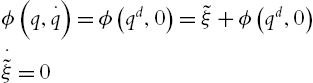
Given a desired time-varying position ![]() , the objective of robot control is to design the input torque u in (5.1) such that the tracking error is
, the objective of robot control is to design the input torque u in (5.1) such that the tracking error is
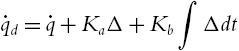
![]() when initial conditions are in arbitrary large domain of attraction. The classic industrial PID law is (5.15). In order to finish the tracking job, we define a filtered error as
when initial conditions are in arbitrary large domain of attraction. The classic industrial PID law is (5.15). In order to finish the tracking job, we define a filtered error as
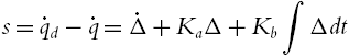
So
We define a matrix ![]() as
as
In order to decouple the PID tracking control (5.19), we choose ![]() , and
, and ![]() as positive definite diagonal matrices. The closed-loop system of the robot (5.1) is
as positive definite diagonal matrices. The closed-loop system of the robot (5.1) is
Using the filtered error s, the final closed-loop equation becomes
where ![]() . The following theorem gives the stability analysis of the PID tracking control.
. The following theorem gives the stability analysis of the PID tracking control.
Theorem 5.3
Proof
Propose the following Lyapunov function:
Using (5.80) the derivative of the proposed function yields
Since ![]() ,
,
Using the PID control law (5.81), then
So
![]() is negative semidefinite on the ball Σ. There exists a ball Σ of radius
is negative semidefinite on the ball Σ. There exists a ball Σ of radius ![]() centered at the origin of the state space on which
centered at the origin of the state space on which ![]() . The origin of the closed-loop equation (5.80) is a stable equilibrium. Since the closed-loop equation is autonomous, we use LaSalle's theorem. Define Ω as
. The origin of the closed-loop equation (5.80) is a stable equilibrium. Since the closed-loop equation is autonomous, we use LaSalle's theorem. Define Ω as

From (5.83), ![]() if and only if
if and only if ![]() . For a solution
. For a solution ![]() to belong to Ω for all
to belong to Ω for all ![]() , it is necessary and sufficient that
, it is necessary and sufficient that ![]() for all
for all ![]() . □
. □
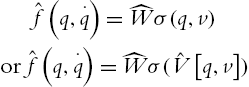
In many cases, in (5.1) the gravity ![]() and the friction
and the friction ![]() are not available. We can use a feedforward neural network to model them as (5.4)
are not available. We can use a feedforward neural network to model them as (5.4)
where ![]() is unknown constant weight,
is unknown constant weight, ![]() is estimated weight, η is the neural approximation error, and σ is a neural activation function. Here, we use the Gaussian function such that
is estimated weight, η is the neural approximation error, and σ is a neural activation function. Here, we use the Gaussian function such that ![]() .
.
This linear-in-the-parameter net is the simplest neural network. According to the universal function approximation theory, the smooth function ![]() can be approximated by a multilayer neural network with one hidden layer in any desired accuracy provided proper weights and hidden neurons:
can be approximated by a multilayer neural network with one hidden layer in any desired accuracy provided proper weights and hidden neurons:
where ![]() ,
, ![]() , m is hidden node number,
, m is hidden node number, ![]() is the weight in a hidden layer. In order to simplify the theory analysis, we first use linear-in-the-parameter net (5.84), then we will show that the multilayer neural network (5.85) can also be used for the neural control of robot manipulators. According to universal function approximation property,
is the weight in a hidden layer. In order to simplify the theory analysis, we first use linear-in-the-parameter net (5.84), then we will show that the multilayer neural network (5.85) can also be used for the neural control of robot manipulators. According to universal function approximation property, ![]() can be shown that as long as x is restricted to a compact set
can be shown that as long as x is restricted to a compact set ![]() . There exist synaptic weights and thresholds such that
. There exist synaptic weights and thresholds such that
The functional approximation error ![]() of the neural network generally decreases as m increases. In fact, for any positive number
of the neural network generally decreases as m increases. In fact, for any positive number ![]() , we can find a feedforward neural network such that
, we can find a feedforward neural network such that
Or
When the unknown dynamic ![]() in (5.84) is big, in order to assure asymptotic stability, the integral gain
in (5.84) is big, in order to assure asymptotic stability, the integral gain ![]() has to be increased. This may cause big overshoot, bad stability, and integrator windup. Model-free compensation is an alternative solution, where
has to be increased. This may cause big overshoot, bad stability, and integrator windup. Model-free compensation is an alternative solution, where ![]() is estimated by a neural network as in (5.84). Normal neural PD control is
is estimated by a neural network as in (5.84). Normal neural PD control is
where ![]() . With the filtered error,
. With the filtered error,
(5.16) becomes
The control (5.91) avoids integrator problems in (5.15). Unlike industrial PID control, they cannot reach asymptotic stability. The stability condition of the neural PD control (5.89) is ![]() , B is a constant. In order to decrease
, B is a constant. In order to decrease ![]() ,
, ![]() has to be increased. This causes a long settling time problem. The asymptotic stability (
has to be increased. This causes a long settling time problem. The asymptotic stability (![]() ) requires
) requires ![]() .
.
An integrator is added into the normal neural PD control (5.89); it has a similar form as the industrial PID in (5.15),
So

The closed-loop system of the robot (5.1) is

where ![]()
here, ![]() . With the filtered error, the final closed-loop equation becomes
. With the filtered error, the final closed-loop equation becomes
The following theorem gives the stability analysis of the neural PID control. From this theorem, we can see how to train the weight of the neural compensator in (5.92).
Theorem 5.4
Proof
We propose the following Lyapunov function:
Using (5.96) and ![]() is skew symmetric, i.e.,
is skew symmetric, i.e.,
the derivative of the proposed function yields
Since ![]() ,
,

Using the adaptation law (5.97), then
By the inequality,
Using (5.101),
Since ![]() is constant,
is constant, ![]() is a negative semidefinite provided that
is a negative semidefinite provided that
Define a ball Σ of radius ![]() centered at the origin of the state space, which satisfies these conditions:
centered at the origin of the state space, which satisfies these conditions:

![]() is negative semidefinite on the ball Σ. There exists a ball Σ of a radius
is negative semidefinite on the ball Σ. There exists a ball Σ of a radius ![]() centered at the origin of the state space on which
centered at the origin of the state space on which ![]() . The origin of the closed-loop equation (5.96) is a stable equilibrium. Since the closed-loop equation is autonomous, we use LaSalle's theorem. Define Ω as
. The origin of the closed-loop equation (5.96) is a stable equilibrium. Since the closed-loop equation is autonomous, we use LaSalle's theorem. Define Ω as
From (5.102), ![]() if and only if
if and only if ![]() . For a solution
. For a solution ![]() to belong to Ω for all
to belong to Ω for all ![]() , it is necessary and sufficient that
, it is necessary and sufficient that ![]() for all
for all ![]() . Therefore it must also hold that
. Therefore it must also hold that ![]() for all
for all ![]() . We conclude that from the closed-loop system (5.96), if
. We conclude that from the closed-loop system (5.96), if ![]() for all
for all ![]() , then
, then

implies that ![]() for all
for all ![]() . So
. So ![]() is the only initial condition in Ω for which
is the only initial condition in Ω for which ![]() for all
for all ![]() . Finally, we conclude from all of this that the origin of the closed-loop system (5.96) is locally asymptotically stable. The tracking error s and its derivative
. Finally, we conclude from all of this that the origin of the closed-loop system (5.96) is locally asymptotically stable. The tracking error s and its derivative ![]() are bounded, which implies boundedness of e and
are bounded, which implies boundedness of e and ![]() . Given that the desired trajectories
. Given that the desired trajectories ![]() and
and ![]() are also bounded, joint position q and joint velocity
are also bounded, joint position q and joint velocity ![]() are bounded. □
are bounded. □
5.4 Experimental results of the neural PID
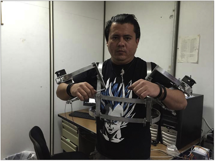
Recently, we construct the portable exoskeleton robot, shown in Fig. 5.1. It has two servomotors. By our special design, it can move freely in 3D space; see Appendix A. The control computer is a Pentium Core2Duo with 2GB of RAM and a 120GB hard disk. The control software is under the operating system Linux Mint 15 “Olivia.” We use this operating system, because the development software has a GNU General Public License. The development environment is Qt4 with C++, which is less runtime in a normal PC, and improves control performance compared with MATLAB Simulink®. Another advantage is that our system can generate executable programs, which can run on any PC without the installing development environment.

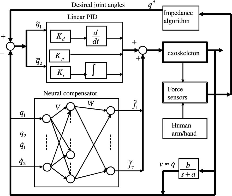
This upper limb exoskeleton is fixed on the human arm. The behavior of the exoskeleton is the same as the human arm; see Fig. 5.2. The exoskeleton is light, and the height can be adjusted for each user. The users left hand is an enable button, which released the brakes on the device and engaged the motor. The reference signals are generated by admittance control in task space. These references are sent to joint space. The robot in joint space can be regarded as free motion without human constraints. The whole control system is shown in Fig. 5.3. The objective of neural PID control is make the transient performance faster with less overshoot, such that human feel comfortable.
All of the controllers employed a sampling frequency of 1 kHz. The two theorems in this paper give sufficient conditions for the minimal values of proportional and derivative gains and maximal values of integral gains. We use (5.45) to estimate the upper and the lower bounds of the eigenvalues of the inertia matrix ![]() , and
, and ![]() in (5.10). We select
in (5.10). We select ![]() ,
, ![]() ,
, ![]() . We choose
. We choose ![]() such that
such that ![]() is satisfied.
is satisfied. ![]() , A is chosen as
, A is chosen as ![]() ,
, ![]() , so
, so ![]() . The joint velocities are estimated by the standard filters:
. The joint velocities are estimated by the standard filters:
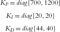
The PID gains are chosen as
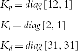
such that the conditions of Theorem 5.2 are satisfied. The initial elements of the weight matrix ![]() are selected randomly from −1 to 1. The active function in (5.26) is a Gaussian function:
are selected randomly from −1 to 1. The active function in (5.26) is a Gaussian function:
where ![]() is selected randomly from 0 to 2. The weights are updated by (5.62) with
is selected randomly from 0 to 2. The weights are updated by (5.62) with ![]() .
.
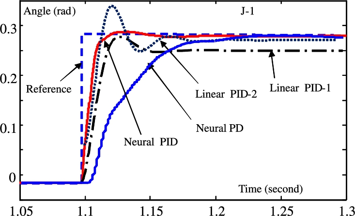
The control results of Joint-1 with neural PID control is shown in Fig. 5.4, marked “Neural PID.” We compare our neural PID control with the other popular robot controllers. First, we use the linear PID (5.15). The PID gains are the same as (5.107), and the control result is shown in Fig. 5.4, marked “Linear PID-2.” Because the steady-state error is so big, the integral gains are increased as
The control result is shown in Fig. 5.4, marked “Linear PID-1,” the transient performance is poor. There still exists regulation error. Further increasing ![]() causes the closed-loop system to be unstable. Then we use a neural compensator to replace the integrator. It is normal neural PD control (5.16). In order to decrease steady-state error, the derivative gains are increased as
causes the closed-loop system to be unstable. Then we use a neural compensator to replace the integrator. It is normal neural PD control (5.16). In order to decrease steady-state error, the derivative gains are increased as
the control result is shown in Fig. 5.4, marked “Neural PD.” The response becomes very slow.
Now we use Joint-2 to compare our neural PID control with the other two types of neural PID control. The control results of these three neural PID controllers are shown in Fig. 5.5. Here, we use a three-layer neural network with three nodes, which have integral, proportional, and derivative properties. A backpropagation like the training algorithm is used to ensure closed-loop stability [29]; it is marked “Neural Net in PID form.” Then we use a one-hidden layer neural network to tune the linear PID gains as in [117]; it is marked “PID tuning via neural net.” It can be found that the “Neural net in PID form” can assure stability, but the transient performance is not good. The “PID tuning via neural net” is acceptable except its slow response.
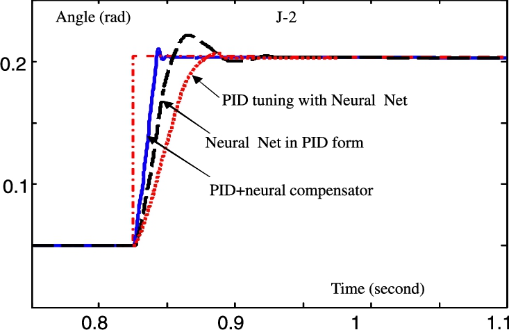
Clearly, neural PID control can successfully compensate the uncertainties such as friction, gravity, and the other uncertainties of the robot. Because the linear PID controller has no compensator, it has to increase its integral gain to cancel the uncertainties. The neural PD control does not apply an integrator, its derivative gain is big.
The structure of the neural compensator is very important. The number of hidden nodes m in (5.5) constitutes a structural problem for neural systems. It is well known that increasing the dimension of the hidden layer can cause the “overlap” problem and add to the computational burden. The best dimension to use is still an open problem for the neural control research community. In this application, we did not use a hidden layer, and the control results are satisfied. The learning gain ![]() in (5.62) will influence the learning speed, so a very large gain can cause unstable learning, while a very small gain produces a slow learning process.
in (5.62) will influence the learning speed, so a very large gain can cause unstable learning, while a very small gain produces a slow learning process.
Now we will carry out some experimental tests by using the neural PID controller in a tracking case. To accomplish this, we will define conveniently the neural gain ![]() , and by using [2]. We obtain the following gain matrices:
, and by using [2]. We obtain the following gain matrices:
The active function in (5.26) is a Gaussian function:
The neural PID tracking control for the first and the second joints are shown in Fig. 5.6 and Fig. 5.7. The position error is reasonably small (between −2 and 2 degrees in both cases). The second joint carries out the extension, the neural network compensates the friction and gravity effects. The actual velocity satisfactorily follows the desired velocity.


Overall, we can notice that, though we have used a small gain ![]() , the robot performance is acceptable when using the neural PID. Unfortunately, we cannot increase too much such gain, since the controller tries to compensate every single disturbance that affects the robot. Then it produces a torque that makes the joints to vibrate continuously. In fact, this vibration affects especially the small joints.
, the robot performance is acceptable when using the neural PID. Unfortunately, we cannot increase too much such gain, since the controller tries to compensate every single disturbance that affects the robot. Then it produces a torque that makes the joints to vibrate continuously. In fact, this vibration affects especially the small joints.
The tracking neural PID control proposed in this paper is compared with the other two types of controllers. We first use normal NN with three-layers, and each layer has 3 nodes. The backpropagation is applied to train the NN. Then we use a one-hidden layer NN to tune the linear PID gains. We find that our neural tracking PID is to ensure stability, but the transient performance is not good, while the PID tuning via neural net is acceptable except for its slow response.
Clearly, neural PID control can successfully compensate the uncertainties such as friction, gravity, and the other uncertainties of the robot. Because the linear PID controller has no compensator, it has to increase its integral gain to cancel the uncertainties. The neural PD control does not apply an integrator, and its derivative gain is big.
5.5 Conclusions
The neural PID proposed in this chapter solves the problems of large integral and derivative gains in the linear PID control and the neural PD control. It keeps good properties of the industrial PID control and neural compensator. Semiglobal asymptotic stability of this neural PID control is proven. When the joint velocities of robot manipulators are not available, local asymptotic stability is assured with filtered positions. The stability conditions give explicit methods to select PID gains. We also apply our neural PID to the exoskeleton robot in CINVESTA-IPN. Theory analysis and experimental study show the validity of the neural PID control.
A novel PID tracking controller is proposed to solve the problem of large integral and derivative gains in the tracking case with linear PID control. Global and semiglobal asymptotic stability of this PID tracking control are proven.