
PID Control in Task Space
Abstract
Task space (or Cartesian space) is defined by the position and orientation of the end-effector of a robot. Joint space is defined by a vector whose components are the translational and angular displacements of each joint of a robotic link. In this chapter, linear PID in the task-space is proposed. The sufficient conditions for asymptotic stability are simple and explicit. The linear PID gains can be selected with these conditions directly. When the measurement of velocities it is not available, a velocity observer (position filter) is applied. The local asymptotic stability of the linear PID control with an observer is proven. The analysis provides explicit conditions for choosing the linear PID gains and the parameters of the velocity observer. We use a 4-DoF (degree-of-freedom) upper limb exoskeleton to verify our PID tuning conditions. The experimental results show that the proposed methodology provides an analytical tool for the robot controller design in the task space.
Keywords
Task space; Linear PID; Semiglobally asymptotic stability
3.1 Linear PID control in task space
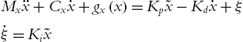
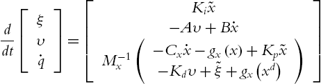
The dynamics of the robot are derived from Euler–Lagrange equation as
where ![]() represents the joint positions.
represents the joint positions. ![]() is the inertia matrix,
is the inertia matrix, ![]() represents centrifugal force,
represents centrifugal force, ![]() ,
, ![]() ,
, ![]() is Christoffel symbols [131], and
is Christoffel symbols [131], and ![]() is the vector of gravity torques.
is the vector of gravity torques.
When the robot's end-effector contacts the environment, or a desired path for the end-effector is specified in task space such as visual space or Cartesian space, a task space coordinate system defined with reference to the environment is convenient for the study of contact motion.
We consider a nonredundant robot. The dimension of the task space is equal to the dimension of the joint space. Let ![]() be a task-space vector defined by
be a task-space vector defined by
where ![]() is the forward kinematics of the robot, which is a nonlinear transformation describing the relation between the joint and task space; x in the task-space is assumed that the robot manipulator is operating in a finite work space such that the Jacobian matrix J is of full rank.
is the forward kinematics of the robot, which is a nonlinear transformation describing the relation between the joint and task space; x in the task-space is assumed that the robot manipulator is operating in a finite work space such that the Jacobian matrix J is of full rank.
Since ![]() the relations between the dynamic models of the task space and the joint space are [75]
the relations between the dynamic models of the task space and the joint space are [75]
where

![]() ,
, ![]() , and
, and ![]() depend on q and
depend on q and ![]() .
.
q and ![]() can be computed from inverse kinematic and
can be computed from inverse kinematic and ![]() . So
. So ![]() ,
, ![]() , and
, and ![]() can be regarded as a function of x and
can be regarded as a function of x and ![]() . The PID attendance control will not use
. The PID attendance control will not use ![]() and
and ![]() , only the following properties will be used to prove stability.
, only the following properties will be used to prove stability.
P3.1. The inertia matrix ![]() is symmetric positive definite, and
is symmetric positive definite, and
where ![]() and
and ![]() are the maximum and minimum eigenvalues of the matrix A.
are the maximum and minimum eigenvalues of the matrix A.
P3.2. For the centrifugal and Coriolis matrix ![]() , there exists a number
, there exists a number ![]() such that
such that
and ![]() are skew symmetric, i.e.,
are skew symmetric, i.e.,
also
P3.3. The gravitational torques vector ![]() and
and ![]() is Lipschitz:
is Lipschitz:
The proof of the above properties is similar with the joint space case [85].
We design a linear stable PID control in task space to regulate the exoskeleton to the desired position. We define the regulation error as
where ![]() is the desired position and orientation of the end-effector.
is the desired position and orientation of the end-effector.
The objective of position control in task space is ![]() and
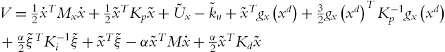
and ![]() when initial conditions are in arbitrary large domain of attraction. A linear PID control in task space law is
when initial conditions are in arbitrary large domain of attraction. A linear PID control in task space law is
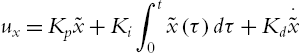
where ![]() ,
, ![]() , and
, and ![]() are proportional, integral, and derivative gains.
are proportional, integral, and derivative gains. ![]() ,
, ![]() . By (3.3) the final control torque applied on each joint is
. By (3.3) the final control torque applied on each joint is
Here, the Jacobian matrix J is known. We do not discuss the case of an uncertain Jacobian matrix [27].
Remark 3.1
Compared with the other task-space PID control, (3.9) has exactly the same form as the classical linear PID control of robot manipulators. In order to prove the stability, in [128] the PID is modified as
where the integral term is changed as ![]() . In [27] the linear PID control is modified as
. In [27] the linear PID control is modified as
where ![]() , the position error
, the position error ![]() is filter by a scalar potential function
is filter by a scalar potential function ![]() . In [40],
. In [40], ![]() is a saturation function.
is a saturation function.
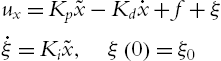
We only discuss the regulation case, i.e., ![]() ,
, ![]() . The PID control law can be expressed via the following equations:
. The PID control law can be expressed via the following equations:
We require that the linear control (3.13) is decoupled, i.e., ![]() , and
, and ![]() are positive definite diagonal matrices. The closed-loop system of the robot (3.2) is
are positive definite diagonal matrices. The closed-loop system of the robot (3.2) is
In matrix form, it is
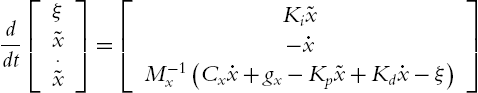
The equilibrium of (3.14) is ![]() . Since at the equilibrium point,
. Since at the equilibrium point, ![]() , the equilibrium is
, the equilibrium is ![]() . In order to move the equilibrium to origin, we define
. In order to move the equilibrium to origin, we define
The closed-loop equation becomes
Theorem 3.1
Proof
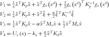
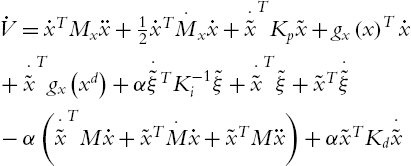
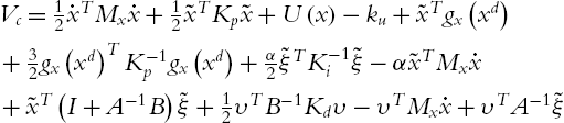
We construct a Lyapunov function as

where ![]() ,
, ![]() ,
, ![]() is added such that
is added such that ![]() . α is a design positive constant.
. α is a design positive constant.
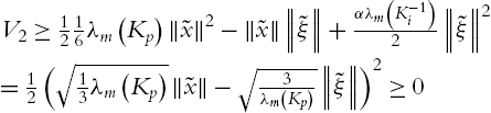
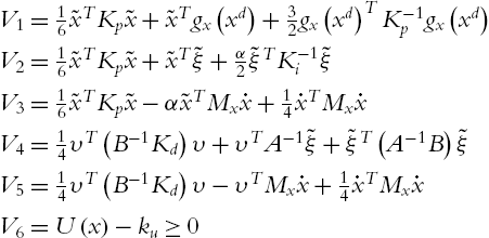
1) We first prove that V is a Lyapunov function, ![]() . The term
. The term ![]() is separated into three parts, and
is separated into three parts, and ![]() :
:
By ![]() ,
, ![]() . It is easy to find
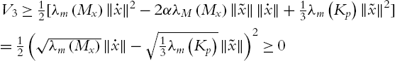
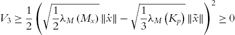
. It is easy to find

When ![]() ,
,
Because
when ![]() ,
,
Obviously, if
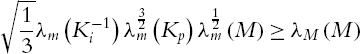
there exists
This means if ![]() is sufficiently large or
is sufficiently large or ![]() is sufficiently small, (3.20) is established, and
is sufficiently small, (3.20) is established, and ![]() is globally positive definite.
is globally positive definite.
2) We now prove ![]() . Using
. Using ![]() ,
, ![]() and
and ![]() , the derivative of V is
, the derivative of V is
Using (3.6), the first three terms of (3.22) become
Because ![]() , and
, and ![]() , the first eight terms of (3.22) are
, the first eight terms of (3.22) are
Now we discuss the last two terms of (3.22). From (3.7), we have
From (3.15),
Since ![]() , using (3.5) and (3.8) the last two terms of (3.22) are
, using (3.5) and (3.8) the last two terms of (3.22) are
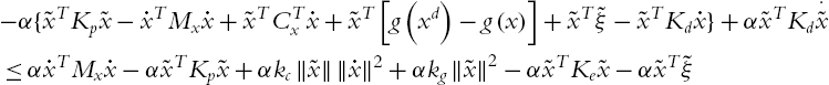

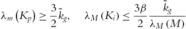
If
and
then ![]() ,
, ![]() decreases. From (3.21), if
decreases. From (3.21), if

then (3.26) is established. Using (3.20) and ![]() , (3.27) is (3.16).
, (3.27) is (3.16). ![]() is negative semidefinite.
is negative semidefinite.
3) Finally, we prove semiglobally asymptotic stability. Define a ball Σ of radius ![]() centered at the origin of the state space, which satisfies these conditions:
centered at the origin of the state space, which satisfies these conditions:
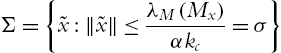
![]() is negative semidefinite on the ball Σ. There exists a ball Σ of radius
is negative semidefinite on the ball Σ. There exists a ball Σ of radius ![]() centered at the origin of the state space on which
centered at the origin of the state space on which ![]() . The origin of the closed-loop equation (3.15) is a stable equilibrium. Since the closed-loop equation is autonomous, we use LaSalle's theorem. Define Ω as
. The origin of the closed-loop equation (3.15) is a stable equilibrium. Since the closed-loop equation is autonomous, we use LaSalle's theorem. Define Ω as
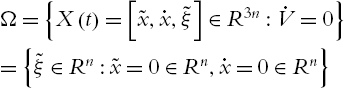
From (3.22), ![]() if and only if
if and only if ![]() . For a solution
. For a solution ![]() to belong to Ω for all
to belong to Ω for all ![]() , it is necessary and sufficient that
, it is necessary and sufficient that ![]() for all
for all ![]() . Therefore it must also hold that
. Therefore it must also hold that ![]() for all
for all ![]() . We conclude that from the closed-loop system (3.15), if
. We conclude that from the closed-loop system (3.15), if ![]() for all
for all ![]() , then
, then

implies that ![]() for all
for all ![]() . So
. So ![]() is the only initial condition in Ω for which
is the only initial condition in Ω for which ![]() for all
for all ![]() .
.
Finally, we conclude from all this that the origin of the closed-loop system (3.15) is locally asymptotically stable. Because ![]() , the upper bound for
, the upper bound for ![]() can be
can be
It establishes the semiglobal stability of our controller, in the sense that the domain of attraction can be arbitrarily enlarged with a suitable choice of the gains. Namely, increasing ![]() the basin of attraction will grow. □
the basin of attraction will grow. □
Remark 3.2
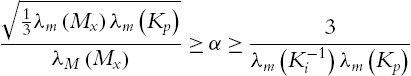
The tuning procedure of the parameters can be calculated from the conditions (3.16). It is more simple than the tuning procedures in [27,40,72,128]. PID controllers are not linear, and the conditions for the PID gains are not explicit. The upper or lower bounds of PID gains need the maximum eigenvalue of ![]() in (3.16), it can be estimated without calculating
in (3.16), it can be estimated without calculating ![]() . For a robot with only revolute joints,
. For a robot with only revolute joints,
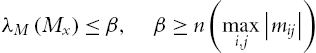
where ![]() stands the ijth element of
stands the ijth element of ![]() ,
, ![]() . A β can be selected such that it is much bigger than all elements.
. A β can be selected such that it is much bigger than all elements.
Remark 3.3
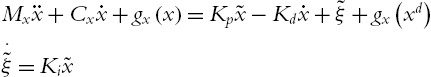
It is well known that without the gravity force ![]() in (3.2), PD control with any positive gains can drive the closed-loop system asymptotic stability. The main objective of the integral action can be regarded to cancel the gravity torque. In order to decrease integral gain, the estimated gravity is applied to the PID control (3.13). The PID control with an approximate gravity compensation
in (3.2), PD control with any positive gains can drive the closed-loop system asymptotic stability. The main objective of the integral action can be regarded to cancel the gravity torque. In order to decrease integral gain, the estimated gravity is applied to the PID control (3.13). The PID control with an approximate gravity compensation ![]() is
is

If we define
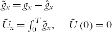
![]() also satisfies Lipschitz condition (3.8)
also satisfies Lipschitz condition (3.8)
The new Lyapunov function in the above proof is
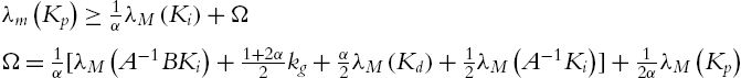
where ![]() . The above theorem is also correct for the PID control with an approximate gravity compensation (3.28). The condition for PID gains (3.16) becomes
. The above theorem is also correct for the PID control with an approximate gravity compensation (3.28). The condition for PID gains (3.16) becomes
where ![]() ,
, ![]() .
.
In a redundant case, for example, ![]() . Define
. Define ![]() to be the task space vector
to be the task space vector
where ![]() is the position and orientation of the end-effector in base coordinates.
is the position and orientation of the end-effector in base coordinates. ![]() is the forward kinematics of the robot, which is a nonlinear transformation describing the relation between the joint and task space. The Cartesian velocity vector
is the forward kinematics of the robot, which is a nonlinear transformation describing the relation between the joint and task space. The Cartesian velocity vector ![]() ,
, ![]() is the linear velocity,
is the linear velocity, ![]() is the angular velocity. Besides the original control task for the end-effector, the joint space of the 7-DoF exoskeleton are also subjected to some constraints, because the exoskeleton is fixed with a human arm. We define one constraint task as
is the angular velocity. Besides the original control task for the end-effector, the joint space of the 7-DoF exoskeleton are also subjected to some constraints, because the exoskeleton is fixed with a human arm. We define one constraint task as
where ![]() is a scalar. The augmented task space is defined as
is a scalar. The augmented task space is defined as

The derivative of x is given as
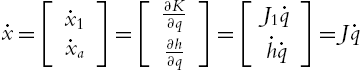
where ![]() is the Jacobian matrix in the augmented task space. In order to design a control which is free of the definition of the augmented task space
is the Jacobian matrix in the augmented task space. In order to design a control which is free of the definition of the augmented task space ![]() , we choose
, we choose ![]() as the null space of
as the null space of ![]() ,
,
where ![]() is a small vector. It is assumed that the exoskeleton is operating in a finite work-space such that J is nonsingular. Since
is a small vector. It is assumed that the exoskeleton is operating in a finite work-space such that J is nonsingular. Since ![]() the relations between the dynamic models of the task space and the joint space are
the relations between the dynamic models of the task space and the joint space are
In the case of the DoF of the robot is less than 6, the demission of the Jacobian will be the same as (3.10).
3.2 Linear PID control with velocity observers
In contrast to the high precision of the position measurements by the optical encoders, the measurement of velocities by tachometers may be quite mediocre in accuracy, specifically for certain intervals of velocity. The common idea in the design of PID controllers, which requires velocity measurements, has been to propose state observers to estimate the velocity. In the PI2D [106], semiglobal asymptotic stability was proved with one additional filtered derivative action.
We will not use ![]() to obtain
to obtain ![]() . A filter/observer will be used to calculate
. A filter/observer will be used to calculate ![]() from
from ![]() . We use a first-order and zero-relative position filter to estimate velocity [85]:
. We use a first-order and zero-relative position filter to estimate velocity [85]:
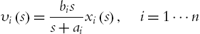
where ![]() is an estimation of
is an estimation of ![]() ,
, ![]() , and
, and ![]() are the elements of diagonal matrices A and B,
are the elements of diagonal matrices A and B, ![]() ,
, ![]() ,
, ![]() ,
, ![]() . The transfer function (3.32) can be realized by
. The transfer function (3.32) can be realized by

The linear PID control (3.13) becomes

where ![]() , and
, and ![]() are positive definite diagonal matrices;
are positive definite diagonal matrices; ![]() and
and ![]() in (3.32) are positive constants.
in (3.32) are positive constants.
The closed-loop system of the robot (3.1) is
The equilibrium of (3.34) is ![]() .
.
Theorem 3.2
Consider the robot dynamic (3.2) controlled by the linear PID controller (3.33). A and B satisfy

where ![]() , the closed-loop system (3.34) is locally asymptotically stable at the equilibrium
, the closed-loop system (3.34) is locally asymptotically stable at the equilibrium ![]() , in the domain of attraction:
, in the domain of attraction:

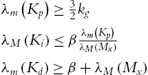
provided that control gains satisfy

where ![]() satisfies (3.8),
satisfies (3.8), ![]() is the condition number of
is the condition number of ![]() .
.
Proof
We construct a Lyapunov function as
where ![]() ,
, ![]() is defined in (3.3),
is defined in (3.3), ![]() is added such that
is added such that ![]() . α is a design positive constant.
. α is a design positive constant.
1) We first prove that ![]() . The term
. The term ![]() is separated into three parts, and
is separated into three parts, and ![]() :
:
Here ![]() and
and ![]() are the same as (3.18), i.e.
are the same as (3.18), i.e.
For ![]() , if
, if ![]()
Because ![]() and
and ![]() , it is easy to find that,
, it is easy to find that,
if ![]() or
or ![]()

If ![]() or
or ![]() ,
,

Because ![]() , obviously there exist α, A, and B such that
, obviously there exist α, A, and B such that

This means if ![]() is sufficiently large or
is sufficiently large or ![]() is sufficiently small, (3.20) is established, and
is sufficiently small, (3.20) is established, and ![]() is globally positive definite.
is globally positive definite.
2) Now we compute the derivative of ![]() :
:

Using (3.34) and (3.6), the first six terms of (3.41) become
The 7th term of (3.41) is

Using ![]() , and
, and ![]() , the terms of 8th–10th of (3.41) are
, the terms of 8th–10th of (3.41) are
The 11th term of (3.41) is

Using (3.5),
Using ![]() and
and ![]() , the last two terms of (3.41) are
, the last two terms of (3.41) are
Combine (3.42), (3.43), (3.44), (3.45), and (3.46)


where ![]() . In order to assure
. In order to assure ![]() in (3.48), we need
in (3.48), we need

Using ![]() , i can be “
, i can be “![]() ” or “
” or “![]() ,” and the last condition of (3.49) can be replaced by
,” and the last condition of (3.49) can be replaced by

It is the attraction area (3.36).
Using ![]() , the second condition of (3.49) is
, the second condition of (3.49) is

It is the condition for ![]() in (3.37).
in (3.37).
The third condition of (3.49) is
It is the condition for ![]() in (3.37). The condition for
in (3.37). The condition for ![]() in (3.37) is obtained from (3.39). The rest part of the proof is the same as Theorem 3.1. □
in (3.37) is obtained from (3.39). The rest part of the proof is the same as Theorem 3.1. □
Remark 3.4
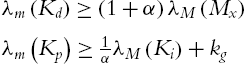
The conditions (3.35) and (3.37) decide how to choose the PID gains. The first condition of (3.37) is
the third condition of (3.37) is ![]() , and they are compatible. When
, and they are compatible. When ![]() is not big, these conditions can be established. The second condition of (3.37) and the third condition of (3.35) are not directly compatible. We first let α as small as possible, and
is not big, these conditions can be established. The second condition of (3.37) and the third condition of (3.35) are not directly compatible. We first let α as small as possible, and ![]() as big as possible. So
as big as possible. So ![]() cannot be big. These requirements are reasonable for our real control. If we select
cannot be big. These requirements are reasonable for our real control. If we select ![]() , form the third condition of (3.35),
, form the third condition of (3.35), ![]() . The second condition of (3.37) requires
. The second condition of (3.37) requires ![]() . There exists
. There exists ![]() and a small α such that
and a small α such that ![]() . After A and B are decided, we use the second condition of (3.37) to select
. After A and B are decided, we use the second condition of (3.37) to select ![]() .
.
3.3 Experimental results
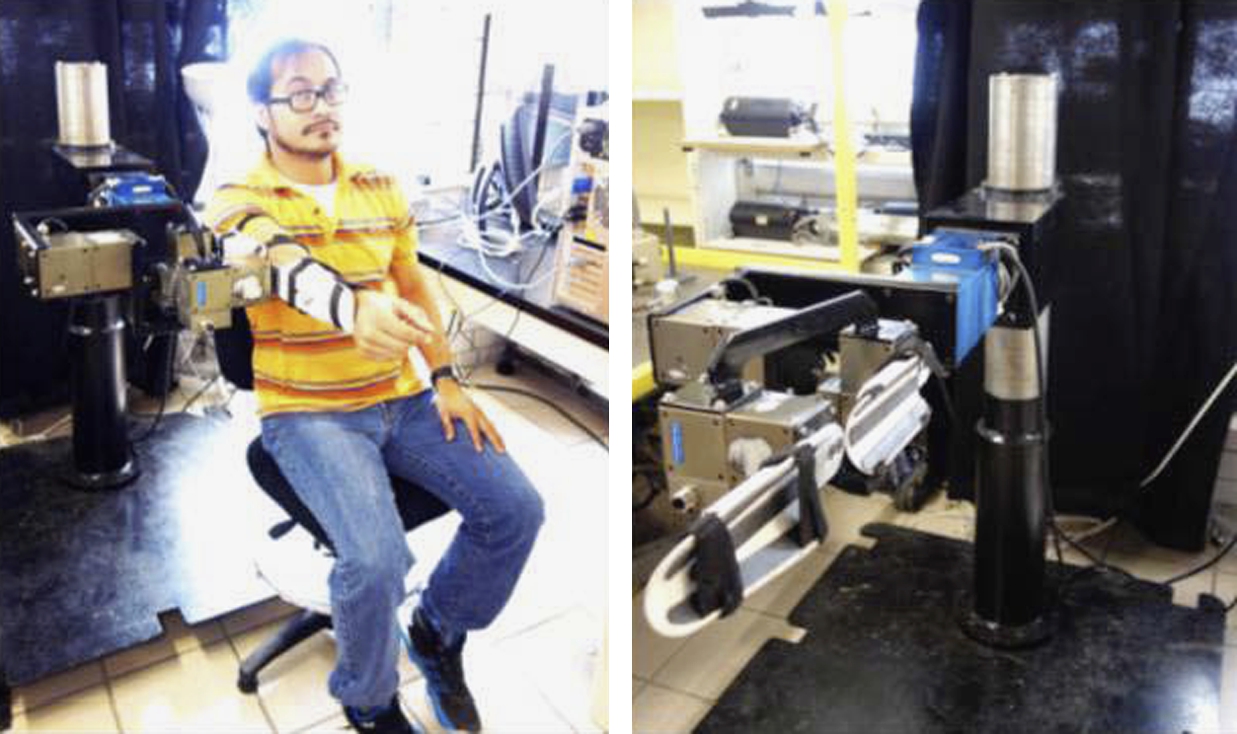
We have constructed the heavy duty exoskeleton robot, CINVESRobot-1, shown in Fig. 3.1. It has a 4-DoF. The computer control platform for our upper limb exoskeleton is an Intel Pentium [email protected] GHz processor and 2GB RAM. The operation software are Windows XP with Matlab 7.2 + WinCon. The real-time control programs are the Real-Time Target.
The running frequency of the CPU processor in each module is a 1.0 GHz processor. The communication rate of the CAN bus is set as 5K bps. We use 500 Hz as the sampling frequency as the control loop. So the sampling/control speed is much lower than the modules and their communication rate. In this way, each module has enough time to finish its job assigned by the upper PC, and send back the positions to the PC. The CAN bus does not have a separate clock signal for synchronization. When the bus is idle, the synchronization starts, and resynchronization occurs on every recessive to dominant transition during the frame. So all nodes on the CAN bus operate at the same bit rate with respect to noise, phase shifts, and oscillator drift.
The users left-hand is an enable button which released the brakes on the device and engaged the motor. We use three types modules for the four joints: PowerCube ![]() ,
, ![]() , and
, and ![]() . The power supply for
. The power supply for ![]() is 48VDC, and for
is 48VDC, and for ![]() and
and ![]() are 24VDC. The normal torques are 142 Nm, 72 Nm, and 23 Nm. The weight of these modules are 5.6 kg, 3.4 kg, and 1.7 kg.
are 24VDC. The normal torques are 142 Nm, 72 Nm, and 23 Nm. The weight of these modules are 5.6 kg, 3.4 kg, and 1.7 kg.
The first joint of the 4-DoF exoskeleton is mounted on the ground. It needs to hold all other joints. The dimension of the exoskeleton is about 1 m. The maximum load for Joint-1 is about 15 kg, i.e., it can other two ![]() and five
and five ![]() modules. The second joint of this exoskeleton uses
modules. The second joint of this exoskeleton uses ![]() module. The third and fourth joints use
module. The third and fourth joints use ![]() module. The Joint-2 can be connected by the other five
module. The Joint-2 can be connected by the other five ![]() modules. Joint-3 can hold 7.8 kg, if the dimensions of Joint-4, Joint-5, etc., are estimated as 0.3 m. So Joint-3 can be connected by another
modules. Joint-3 can hold 7.8 kg, if the dimensions of Joint-4, Joint-5, etc., are estimated as 0.3 m. So Joint-3 can be connected by another ![]() modules.
modules.
We use the following task space controller to regulate the robot position x such that x can follow ![]() :
:
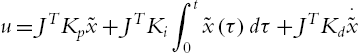
where ![]() .
.
The two theorems in this chapter give sufficient conditions for the minimal values of proportional and derivative gains and maximal values of integral gains. We use the above parameters to estimate the upper and lower bounds of the eigenvalues of the inertia matrix ![]() , and
, and ![]() in (3.8), i.e.,
in (3.8), i.e., ![]() ,
, ![]() ,
, ![]() . We choose
. We choose ![]() such that
such that ![]() is satisfied. We select
is satisfied. We select ![]() ; A is chosen as
; A is chosen as ![]() ,
, ![]() , so
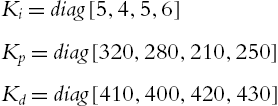
, so ![]() . The gains of the PID controller in task space are
. The gains of the PID controller in task space are
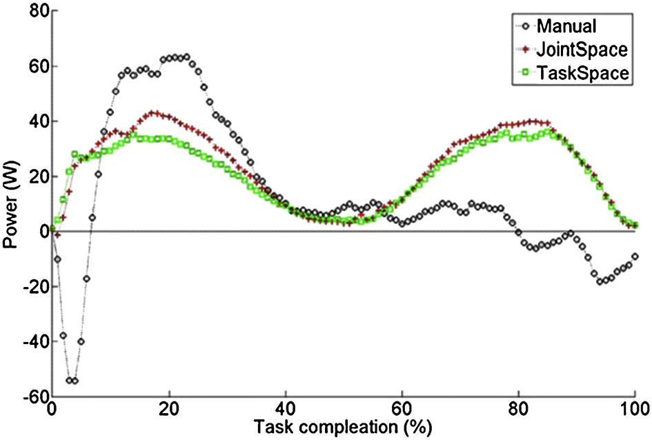
Each control scheme moved to each target once in random order. Four repetitions were repeated for each subject. A total of 395 trails were recorded consisting of 118 trials for manual control, 134 trials for joint space control, and 143 trials for task space. Since the exact positions in task space are not available (in fact we do not have a visual system), we cannot compare the position regulation errors in the task space. We use the power exchange, defined by the product of the recorded force/torque and its respective velocity at each sensor, as an index to evaluate the task space control. The less power the controller used, the better the controller is.
Fig. 3.2 shows the average power exchange for manual control, joint space PID control and task space PID control after they have been normalized with respect to time.
The energy exchange, which is between the exoskeleton and subject was calculated for each trial by integrating the power. Additionally, the negative and positive components of the energy were each computed separately. Table 3.1 shows the mean energy for all trials with its ![]() confidence interval.
confidence interval.
Table 3.1
Energy exchange
| Manual | Joint Space | Task Space | |
|---|---|---|---|
| Total | 9.29 ± 1.11 | 19.55 ± 1.04 | 17.43 ± 1.01 |
| Negative | −6.92 ± 0.34 | −0.25 ± 0.34 | −0.098 ± 0.33 |
| Positive | 16.21 ± 1.10 | 19.81 ± 1.03 | 17.52 ± 0.99 |

We can see that
1) the energy power exchange: manual control has a sharp drop with a negative power peaking about ![]() , followed by a steep increase to a positive power of around
, followed by a steep increase to a positive power of around ![]() and finally has a decline to around
and finally has a decline to around ![]() . The sharp decrease is due to the device falling slightly after the breaks are disengaged. Joint and task space control have a similar rise and fall on the power curve but without the initial drop as the controllers prevented the exoskeleton from falling when the breaks were released. As the subject lowers the arm, gravity pulls it in the same direction as the motion creating a very low power.
. The sharp decrease is due to the device falling slightly after the breaks are disengaged. Joint and task space control have a similar rise and fall on the power curve but without the initial drop as the controllers prevented the exoskeleton from falling when the breaks were released. As the subject lowers the arm, gravity pulls it in the same direction as the motion creating a very low power.
2) Energy: the total energy for manual control is lowest for all the controllers. Because the task space PID control has almost no negative power, we would expect them to have a higher energy than the manual control.
The second experiment is to draw several “8.” In order to control the 4-DoF exoskeleton, we use three forces ![]() and one torque
and one torque ![]() as the input
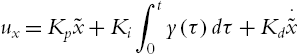
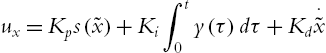
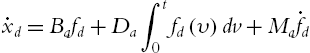
as the input ![]() . The admittance control is to generate desired trajectories of the four joints from
. The admittance control is to generate desired trajectories of the four joints from ![]() , and to move the end-effector of the exoskeleton robot from an initial position into a desired position. The PID admittance control in task space is
, and to move the end-effector of the exoskeleton robot from an initial position into a desired position. The PID admittance control in task space is
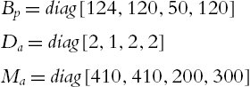
where ![]() ,
, ![]() , and
, and ![]() are human impedance parameters, which depend on each one's feelings. In this paper, we select
are human impedance parameters, which depend on each one's feelings. In this paper, we select
Here, the forces ![]() generate three-dimension trajectories
generate three-dimension trajectories ![]() , while the torque
, while the torque ![]() gives the orientation of the end-effector; see Fig. 3.3.
gives the orientation of the end-effector; see Fig. 3.3.

The trajectory of the end-effector in the tasks pace is shown in Fig. 3.4. Here, the trajectory in 3D space is calculated from forward kinematic of the exoskeleton, because we do not have effective 3D motion tracking system to show it.

We can see that the upper limb exoskeleton can be controlled by a force sensor, and move freely. It can draw an “8” within 6 seconds. The accuracy of the movement depends on the human model, i.e., the human has to transfer a 3D “8” into corresponding forces.
3.4 Conclusions
In this chapter, the classical linear PID is applied for the exoskeleton robot control in task space. We analyze classic linear PID control in the task space. The semiglobal and local asymptotic stability conditions are more simple than the others, and these conditions give an explicit method to decide the PID gains in the task space. The above new approaches are successfully applied to the CINVESTAV 4-DoF exoskeleton robot.