Patrick Bangert Artificial Intelligence Team, Samsung SDS America, San Jose, CA, United States algorithmica technologies GmbH, Küchlerstrasse 7, Bad Nauheim, Germany
Abstract
The field of machine learning is introduced at a conceptual level. Ideas such as supervised and unsupervised as well as regression and classification are explained. The tradeoff between bias, variance, and model complexity is discussed as a central guiding idea of learning. Various types of model that machine learning can produce are introduced such as the neural network (feed-forward and recurrent), support vector machine, random forest, self-organizing map, and Bayesian network. Training a model is discussed next with its main ideas of splitting a dataset into training, testing, and validation sets as well as performing cross-validation. Assessing the goodness of the model is treated next alongside the essential role of the domain expert in keeping the project real. The chapter concludes with some practical advice on how to perform a machine learning project.
Keywords
machine learning
artificial intelligence
neural network
support vector machine
random forest
self-organizing map
Bayesian network
bias-variance tradeoff
cross-validation
goodness of fit
In this chapter, we give an introduction to machine learning, its pivotal ideas, and practical methods as applied to industrial datasets. The dataset was discussed in the previous chapter and so here we assume that a clean dataset already exists alongside a clear problem description. Some principal ideas are introduced first, after which we discuss some different model types, and then discuss how to assess the quality and fitness-for-purpose of the model.
3.1. Basic ideas of machine learning
Machine learning is the name given to a large collection of diverse methods that aim to produce models given enough empirical data only. They do not require the use of physical laws or the specification of machine characteristics. They determine the dependency of the variables among each other by using the data, and only the data.
That is not to say that there is no more need for a human expert. The human expert is essential but the way the expertise is supplied is very different to the first principles model. In machine learning, domain expertise is supplied principally in these four ways:
1. Providing all relevant variables and excluding all irrelevant variables. This may include some elementary processed variables via feature engineering, for example, when we know that the ration between two variables is very relevant, we may want to explicitly supply that ratio as a column in the data table.
2. Providing empirical data that is significant and representative of the situation.
3. Assessing the results of candidate models to make sure that they output what is expected.
4. Explicitly adding any essential restrictions that must be obeyed.
These inputs are important, but they are easily supplied by an expert who knows the situation well and who knows a little about the demands of data science.
The subject of machine learning has three main parts. First, it consists of many prototypical models that could be applied to the data at hand. These are known by names such as neural networks, decision trees, or k-means clustering. Second, each of these comes with several prescriptions, so called algorithms that tell us how to calculate the model coefficients from a data set. This calculation is also called training the model. After training, the initial prototype has been turned into a model for the specific data set that we provided. Third, the finished model must be deployed so that it can be used. It is generally far easier and quicker to evaluate a model than to train a model. In fact, this is one of the primary features of machine learning that make it so attractive: Once trained, the model can be used in real-time. However, it needs to be embedded in the right infrastructure to unfold its potential.
Associated to machine learning are the two essential topics that are at the heart of data science. First, the data must be suitably prepared for learning, which we discussed in Chapter 2. Second, the resultant model must be adequately tested, and its performance must be demonstrated using rigorous mathematical means. This pre-processing and post-processing before and after machine learning is applied to round out the scientific part of a data science project. In addition to these scientific parts, there are managerial and organizational parts that concern collecting the data and dealing with the stakeholders of the application.
In this book, we will treat all these topics, except the training algorithms. These form the bulk of the literature on machine learning and are technically challenging. This book aims to provide an overview to the industrial practitioner and not a university course on machine learning. The practitioner has access to various computer programs that include these methods and so a detailed understanding of how a model is trained is not necessary. On the other hand, it is essential that a practitioner understand what must be put into such a training exercise and how to determine whether the result is any good. So, this will be our focus.
Methods of machine learning are often divided into two groups based on two different attributes. One grouping is into supervised and unsupervised methods. The other grouping is into classification and regression methods.
Supervised methods deal with datasets for which we possess empirical data for the inputs to the model as well as the desired outputs of the model. Unsupervised methods deal with datasets for which we only have the inputs. Imagine teaching a child to add two numbers together. Supervised learning consists of examples like and whereas unsupervised learning consists of examples like and . It is clear from this difference that we can expect supervised methods to be much more accurate in reproducing the outcome. Unsupervised methods are expected to learn the structure of the input data and recognize some patterns in them.
Fig. 3.1 illustrates the difference in the context of learning the difference between two collections of data points. In the first example, we know that circles and triangles are different and must learn where to divide the dataspace between them. In the second example, we only have points and must learn that they can be meaningfully divided into two clusters such that points in one cluster are maximally similar and points in different clusters are maximally different from each other—for some measure of similarity that makes sense in the context of the problem domain.
Figure 3.1An illustration of the difference between supervised and unsupervised learning.
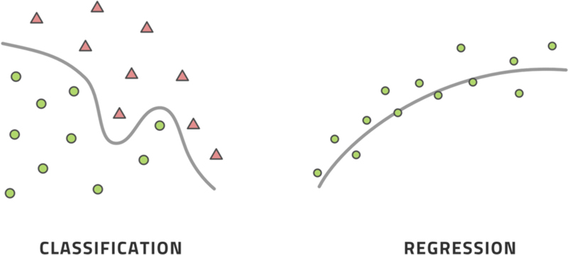
The difference between classification and regression methods is similarly fundamental. Classification methods aim to place a datapoint into one of several groups while regression methods aim to compute some numerical value. Fig. 3.2 illustrates the difference. In the first example, we only wish to draw a dividing line between the circles and the triangles, differentiating one category from the other. In the second example, we want to reproduce a continuous numeric value as accurately as possible.
Figure 3.2An illustration of the difference between classification and regression methods.
This distinction is closely related to the difference between a categorical variable and a continuous variable. A categorical variable is equal to one of several values, like 1, 2, or 3, where the values indicate membership in some group. The difference between two values is therefore meaningless. If datapoint A has value 3 and datapoint B has value 2, all this means is that A belongs to group 3 and B belongs to group 2. Taking the difference of the values, , has no meaning, that is, the difference between the two datapoints does not necessarily belong to group 1 nor does group membership necessarily even make sense for the difference.
A continuous variable is different in that it measures a quantity and taking the difference does mean something real. For instance, if datapoint A has a flow rate of 1 ton per hour and datapoint B has a flow rate of 2 tons per hour, we can take the difference and the difference is 1 ton per hour of flow, which is a meaningful quantity that we can understand.
Machine learning has many methods and all methods are either supervised or unsupervised, and either classification or regression. Any task that uses machine learning can also be divided into these categories. These two groupings are the first point of departure in selecting the right method to solve the problem at hand. So, ask yourself:
1. Do you have data for the result you want to compute, or only for the factors that go into the computation?
2. Is the result a membership in some category, or a numerical value with intrinsic meaning?
We will present methods for all these possibilities guided by the state-of-the-art and industrial experience. This book will not present an exhaustive list of all possible methods as this would go well beyond our scope.
As we need to be brief on the technical aspects of machine learning, here are some great books for further reading on machine learning in and of itself. A great book on the ideas of machine learning without diving into its technical depths is Domingos (2015). If you are more interested in the general economic ramifications of the field, an excellent presentation is in Agrawal, Gans, and Goldfarb (2018). More mathematical books that present a great overview are Mitchell (2018), Bishop (2006), MacKay (2003), and Goodfellow, Bengio, and Courville (2016).
3.2. Bias-variance complexity trade-off
One of the most important aspects in machine learning concerns the quality of the model that you can expect, given the quality of the data you have to make the model. Three aspects of the model are important here.
The bias of the model is an assessment of how far off the average output of the model is from the average expected output. The variance of the model is the extent to which inputs that are very close to each other result in outputs that are far from each other. The complexity of the model is generally measured by the number of parameters that must be determined using a machine learning algorithm from the empirical data provided for training.
The concepts of bias and variance are depicted in Fig. 3.3. Imagine throwing darts at a target. If the darts are all close together, the variance is low. If the darts are, on average, close to the center of the target, the bias is low. Of course, we want a model with low bias and low variance.
Figure 3.3The concepts of bias and variance illustrated by throwing darts at a target.
In order to get such a model, we first choose a type of model, that is, a formula with unknown parameters for which we believe that it can capture the full dynamics of our dataset if only the right values for the parameters are found. An example of this is the straight-line model that naturally has two parameters for one independent variable. We shall meet several other models later on that are more expressive because they have more parameters. Having thought about the straight-line, we can easily understand that a quadratic polynomial (three parameters for one independent variable) can model a more complex phenomenon than a straight-line.
Choosing a model that has very few parameters is not good because it will not be able to express the complexity present in the dataset. The model performance in bias and variance will be poor because the model is too simple. This is known as underfitting.
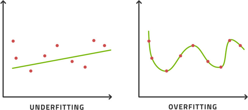
However, choosing a very complex model with a great many parameters is not necessarily the solution because it may get so expressive that it can essentially memorize the dataset without learning its structure. This is an interesting distinction. Learning something suggests that we have understood some underlying mechanism that allows us to do well on all the examples we saw while learning, and any other similar tasks that we have not seen while learning. Memorization will not do this for us and so it is generally thought of as a failed attempt to model something. It is known as overfitting. See Fig. 3.4 for an illustration of underfitting and overfitting.
Figure 3.4If the model is too simple, we will underfit. If the model is very complex, it will overfit.
There must exist some optimal number of parameters that is able to capture the underlying dynamics without being able to simply memorize the dataset. This is some medium number of parameters.
If the model reproduces the data used in its construction poorly, then the model is definitely bad, and this is usually either underfitting or a lack of important data. The fix is to either use a more complex model, to get more data points, or to search for additional independent variables (additional sources of information). The data used in the construction of the model is the training data and the difference between the model output and the expected output for the training data is the training error.
To properly assess model performance, we cannot use the training data, however. We must use a second dataset that was not used to construct the model. This is the testing data that results in a testing error. The testing data is often known as validation data. More complex training algorithms need two datasets, one to train on and another to assess when to stop training. In situations like this, we may need to create three datasets and these are then usually called training, testing, and validation datasets where the testing dataset is used to assess whether training is done and the validation dataset is used to assess the quality of the model.
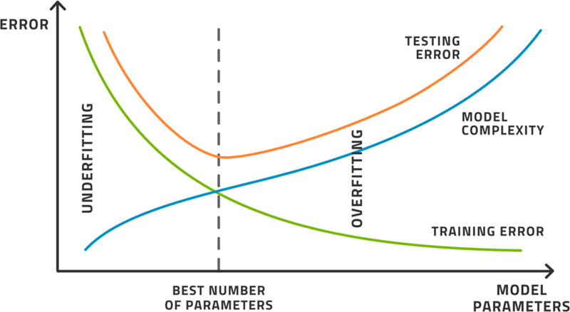
Fig. 3.5 displays the typical model performance as a function of the model complexity. As the model gets more complex, the training error decreases. The testing error decreases at first and then increases again as the model starts to overfit. There is a point, at minimum testing error, when the model achieves its best performance. This is the performance as measured by the bias, that is, the deviation between computed and expected values. This has not yet taken the variance into account. Often, we find that to get better variance, we must sacrifice some bias and vice-versa. This is the nature of the bias-variance-complexity trade-off.
Figure 3.5As the model gets more complex, the training and testing errors change, and this indicates an optimal number of parameters.
While this picture is typical, we usually cannot draw it in practice as each point on this image represents a full training of the model. As training is usually not a deterministic process, the training must be repeated several times for each sample complexity to get a representative answer. This is also needed to measure the variance. It is, in most practical situations, an investment of time and effort no one is prepared to make.
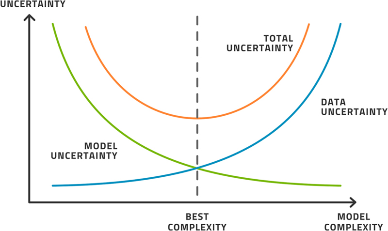
A similar diagram, see Fig. 3.6, can be drawn in terms of variance. There are two major sources of uncertainty in machine learning. First, the uncertainty inherent in the dataset and the manner in which it was obtained. This includes both the method of measurement and the managerial process of selecting which variables to include in the first place. Second, the uncertainty contained in the model and the basic ability of it to express the underlying dynamics of the data. There is a similar compromise that must happen.
Figure 3.6As model complexity rises, model uncertainty decreases but data uncertainty increases. There is an optimal point in the middle.
In the end, we must choose the right model type and the right number of parameters for this model to achieve a reasonable compromise between bias and variance, avoiding both underfitting and overfitting. To prove to ourselves and other that all this has been done, we need to examine the performance on both training and testing data.
3.3. Model types
There are many types of model that we can choose from. This section will explore some popular options briefly with some hints as to when it makes sense to use them. To learn more about diverse model types and machine learning algorithms, we refer to Goodfellow et al. (2016).
3.3.1. Deep neural network
The neural network is perhaps the most famous and most used technique in the arsenal of machine learning (Hagan, Demuth, & Beale, 1996). The recent advent of deep learning has given new color to this model type through novel methods of training its parameters. Training methods are beyond the scope of this book, however.
While it took its inspiration from the network of neurons in the human brain, the neural network is merely a mathematical device. A schematic diagram like the one shown in Fig. 3.7 is commonly displayed for neural networks. On the left side, the input vector enters the network. This is called the input layer and has several neurons equal to the number of elements in the input vector. On the right side, the output vector exits from the network. This is called the output layer and has several neurons equal to the number of elements in the output vector; this is the result of the calculation. In between them are several hidden layers. The number of hidden layers and the number of neurons in each are up to us to choose and is referred to as the topology of the neural network.
Figure 3.7Schematic illustration of a deep neural network.
In bringing the data from one layer to the next, we multiply it by a matrix, add a vector, and apply a so-called activation function to it. These are the parameters for each layer that the machine learning algorithm must choose from the data so that the neural network fits to the data in the best possible way. A neural network with two hidden layers, therefore, looks like
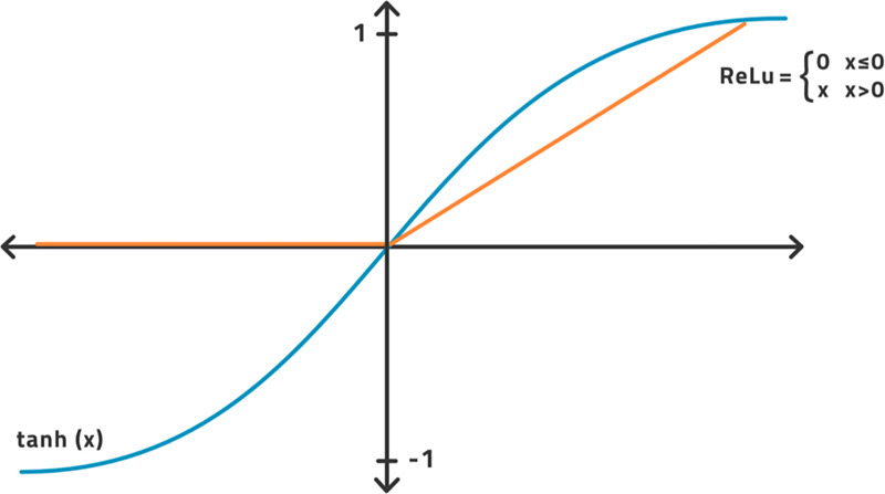
The activation function is not learnt but decided on beforehand. Considerable research has been put into this choice. While older literature prefers , we now have evidence that performs significantly better in virtually all tasks for all layers except the outermost for which we usually choose the identity function. They are both displayed in Fig. 3.8.
Figure 3.8Two popular activation functions for a neural network.
The neural network is not some magical entity. It is the above equation. After we choose values for the parameter matrices and vectors , the neural network becomes a specific model. The main reason it is so famous is that it has the property of universal approximation. This property states that the formula can represent any continuous function with arbitrary accuracy. There are other formulae that have this property, but neural networks were the first ones that were practically used with this feature in mind. In practice, this means that a neural network can represent your data. What the property does not do is tell us how many layers and how many neurons per layer to choose. It also does not tell us how to find the correct parameter values so that the formula does in fact represent the data. All we know is that the neural network can represent the data.
Machine learning as a research field is largely about designing the right learning algorithms, that is, how to find the best parameter values for any given dataset. There are multiple desiderata for it, not just the quality of the parameter values. We also want the training to be fast and to use little processing memory so that training does not consume too many computer resources. Also, we want it to be able to learn from as few examples as possible. Beyond the hype of “big data,” there is now significant research into “small data.”
Many practical applications provide a certain amount of data. Getting more data is either very difficult, expensive, or virtually impossible. In those cases, we cannot get out of machine learning difficulties by the age-old remedy of collecting more data. Rather, we must be smarter in getting the information out of the data we have. That is the challenge of small data and it is not yet solved. We mention it here to put the property of universal approximation into proper context. It is a nice property to be sure, but it has little practical value.
The neural network is the right model to use if the empirical observations are independent of each other. For example, if we take a manual fluid sample from a well once per day and perform a laboratory analysis on it, we can assume that today's observation is largely independent of yesterday's observation but may well depend on the pressure and temperature right now. In this context, we may use pressure and temperature as inputs and expect the neural network to represent the laboratory measurement.
If, however, time delays do play a role, then we must incorporate time into the model itself. Let's say we change the choke setting on a well and measure its wellhead pressure, we will see that the wellhead pressure responds to our action a few minutes later. If we measure these quantities every minute, then the observations are not independent of each other because the observation a few minutes ago causally brought about the current observation. Applying the neural network to such datasets is not a good idea because the neural network cannot represent this type of correlation. For this, we need a recurrent neural network.
3.3.2. Recurrent neural network or long short-term memory network
A recurrent neural network is very similar in spirit to the regular, the so-called feed-forward, neural network. Instead of having connections that move strictly from left to right in the diagram, it also include connections that amount to cycles, see Fig. 3.9. These cycles act as a memory in the formula by retaining—in some transformed way—the inputs made at prior times.
Figure 3.9Schematic illustration of a recurrent neural network.
As mentioned in the previous section, the purpose of recurrence is to model the interdependence between successive observations. In practice such interdependence is virtually always due to time and represents some mechanism of causation or control. If my foot touches the brake pedal in my car, the car slows down a short time later. Modeling the dependence of car speed on the position of the brake pedal can lead to important models, that is, the advanced process control behind the automatic braking system in your car. The time delay involved is important as the car will have moved some distance in that time and so braking must begin sufficiently early so that the car stops before it hits something. It is cases such as this for which the recurrent neural network has been developed.
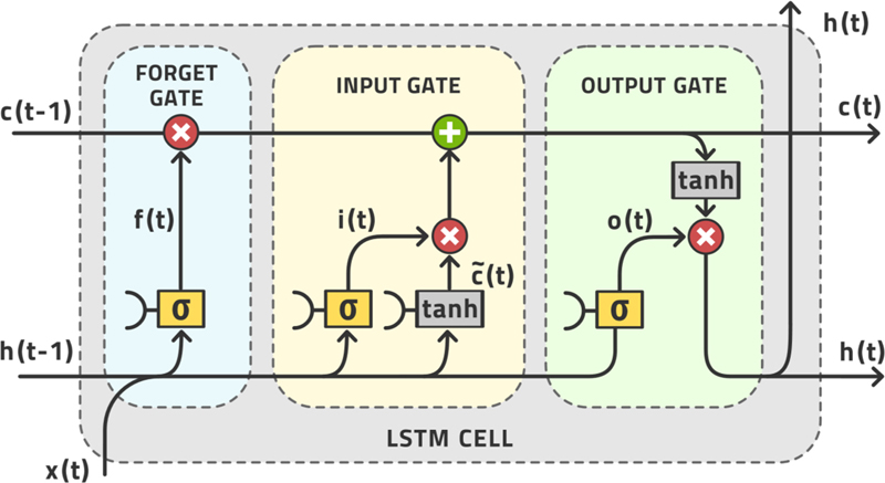
There are many different forms of recurrent neural networks differing mainly in how the cycles are represented in the formula. The current state-of-the-art is the long short-term memory network, or LSTM (Hochreiter and Schmidhuber, 1997; Yu, Si, Hu, & Zhang, 2019; Gers, 2001). This network is made up of cells. A schematic of one cell is shown in Fig. 3.10. These cells can be stacked both horizontally and vertically to make up an arbitrarily large network of cells. Once again, it is up to the human data scientist to choose the topology of this network.
Figure 3.10Schematic illustration of one cell in an LSTM network.
The inner working of one cell is defined by the following equations that refer to Fig. 3.10.
The various and are the weight and bias parameters of the LSTM cell. All weights and biases of the entire network must be tuned by the learning algorithm. The evolution of the internal state of the network is the memory of the network that can encapsulate the time dynamics of the data.
The network is trained by providing it with a time-series for many successive values of time . The model outputs the same time-series but at a later time , where is the forecast horizon. This is the essence of how LSTM can forecast a time-series,
It is generally not a good idea to model the next timestep and then to chain the model
because this compounds errors and makes for a very unreliable model if we want to predict more than one or two timesteps into the future. It is much better to choose the forecast horizon to be some larger number of timesteps. Having done that, the intermediate values can always be computed using the same model with input vectors from earlier in time.
3.3.3. Support vector machines
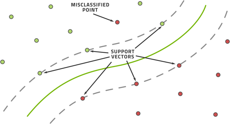
The support vector machine (SVM) is a technique mainly used for classification both in a supervised and unsupervised manner and can be extended to regression as well (Cortes & Vapnik, 1995). The idea, as illustrated in Fig. 3.11 is that we have a set of points that belong to one of two categories and we draw a non-linear plane through the space dividing the data into two pieces. Everything above the plane is classified as one category and everything below the plane is classified as the other. The plane itself is an interpolated spline-like object that is based on a few selected data points—the support vectors—that must be found.
Figure 3.11A support vector machine draws a line through a dataset dividing one category from another as efficiently as possible.
The plane chosen is that which has the maximum distance from all points possible. The points at the boundary of this space form the support vectors. In practice, the classification problem may require multiple planes for a good result. As the space of all points gets divided into sections by a collection of planes, we may find that a few data points are isolated in one area. This is another way of identifying outliers.
3.3.4. Random forest or decision trees
The decision tree is familiar perhaps from management classes where it is used to structure decision making. At the base of the tree is some decision to be made. At each branching, we ask some question that is relatively easy to answer. Depending on the answer, we go down one branch as opposed to another and eventually reach a point on the tree that has no more branches, a so-called leaf node. This leaf node represents the right answer to the original decision.
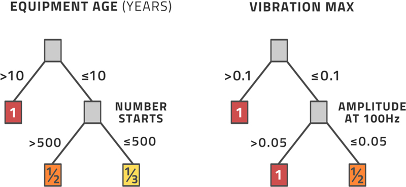
Fig. 3.12 illustrates this using a toy example. The question is whether the equipment needs maintenance or not. The left-hand tree starts by analyzing the equipment age in years. If this is larger than 10 years, we go down the left-hand path and otherwise the right-hand path. The left-hand path terminates at a leaf node with the value 1. The right-hand path leads to a secondary question where we ask for the number of starts of the equipment. If this is larger than 500, we go down that left-hand path leading us to the number 1/2 and otherwise we go down the right-hand path leading to the number 1/3. The number that we end up with is just a numerical score for now.
Figure 3.12An example of two decision trees that can be combined into a random forest.
The numerical score now needs to be interpreted, which is usually done by thresholding, that is, if the score is greater than some fixed threshold, we decide that the equipment needs preventative maintenance and otherwise we decide that it can operate a little longer without inspection. This is an example of a decision tree in the industrial context (Breiman, Friedman, Olshen, & Stone, 1984).
We can combine several decision trees into a single decision-making exercise. Fig. 3.12 displays a second tree that operates in the same way. Having gone through all the trees, we add up the scores and threshold the final result. If the left tree leads to ½ and the right tree leads to 1, then the total is a score of 3/2. This combination of several decision trees is called a random forest.
Constructing the trees, their structures, the decision factors at each branching, and the values for each branching are the model parameters that must be learnt from data. There are sophisticated algorithms for this that have seen significant evolution in recent years making random forest one of the most successful techniques for classification problems. Incidentally, the forest is far from random, of course. The forest is carefully designed by the learning method to give the best possible classification result possible. Random forests can also be used for regression tasks, but they seem to be better suited to classification tasks.
3.3.5. Self-organizing maps (SOM)
A self-organizing map (SOM) is an early machine learning technique that was invented as a visualization aid for the human expert (Kohonen, 2001). Roughly, it belongs to the classification kind of techniques as it groups or clusters data points by similarity. The idea is to represent the dataset with special points that are constructed by the learning method in an iterative manner. These special points are mapped on a two-dimensional grid that usually has the topology of a honeycomb. The topology is important because the learning, that is, the moving around of the special points, occurs over a certain neighborhood of the special point under consideration.
When this process has converged, the special points are arrayed in the topology in a certain way. Any point in the dataset is associated with the special point that it is closest to in the sense of some metric function that must be defined for the problem at hand. This generates a two-dimensional distribution of the entire data. It is now usually a task for the human expert to look at this distribution and determine to what extent the cells in the topology (the honeycomb cells) are similar to each other. Frequently it turns out that several cells are very similar and can be associated with the same macroscopic phenomenon.
For example, in Fig. 3.13 we begin with a topology of 22 honeycomb cells. Having done the learning and the human examination, it is determined that there are only four macroscopically relevant clusters present. Each cluster is represented by several cells. These cells can either have a more subtle meaning within the larger group, or they can simply be a more complex representation of a single cluster than one special point; as one would do using algorithms like k-means clustering (Seiffert & Jain, 2002).
Figure 3.13An example of a self-organizing map.
Ultimately, when one encounters a new data point, one would compute the metric distance between it and all the special points learnt. The special point closest to the new point is its representative and we know which cluster it belongs to. The SOM method has turned out to be a very good classification method in its own right. In addition to this however, the current position of a system can be plotted on the graphic and one can see the temporal evolution on the state chart, which is an elegant visual aid for any human working with the data source.
3.3.6. Bayesian network and ontology
Bayesian statistics follows a different philosophy than standard statistics and this has some technical consequences (Gelman, Carlin, Stern, & Rubin, 2004). Without going into too much detail, standard statistics assesses the probability of an event by the so-called frequentist approach. We will need to collect data as to how frequently this event occurs and does not occur. Usually, this is no problem but sometimes the empirical data is hard to come by, events are rare or very costly, and so on.
Bayesian statistics concerns itself with the so-called degree of belief. This encapsulates the amount of knowledge that we have. If we manage to gather additional knowledge, then we may be able to update our degree of belief and thereby sharpen our probability estimate. The probability distribution after the update is called the posterior distribution. There is a specific rule, Bayes theorem, on how to perform this updating and there is no doubt or difficulty in its application. The tricky part is establishing the probability distribution at the very beginning, the prior distribution. Usually we assume that all events are equally likely if we have no knowledge at all or we might prime the probabilities using empirical frequencies if we do have some knowledge.
Supposing that we have gathered quite a bit of knowledge about the general situation, we can start to create multiple conditional probability distributions. These are conditional on knowing or not knowing certain information.
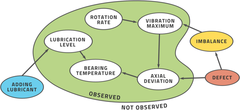
Let's take the case of a root-cause analysis for a mechanical defect in a gas turbine, see Fig. 3.14. We know from past experience that certain measurements provide important information relating to the root cause of this problem, for example, the axial deviation, which is the amount of movement of the rotor away from its engineered position. This, in turn, is influenced by the bearing temperature and the maximum vibration. These two factors are influenced by other factors in turn. We can build up a network of mutually influencing events and factors. At one end of this matrix are the events we are concerned about such as the mechanical defect. At the other end are the events we can directly cause to happen such as the addition of lubricant into the system.
Figure 3.14A very simple example of a Bayesian network for deciding on the root cause of a mechanical defect in a turbine.
Based on our past experience we can establish that if the maximum vibration is above a certain limit, the chance of a rotor imbalance increases by a certain amount, and so on for all the other factors. We can then use statistics to obtain a conditional probability distribution for the mechanical defect as a function of all the factors. This cascading matrix of conditional probabilities is called a Bayesian network (Scutari and Denis, 2015). Once we have this network, it can be used like so: Initially, the chance of a mechanical defect is very small; we assess this from the frequency of observations of such defects. Then we encounter a high bearing temperature and a high vibration for a low rotation rate. Combining this information using the various conditional probabilities updates our probability of defect. If this is sufficiently high, we may release an alarm and give a specific probability for a problem. We can also compute what effect it would have on the probability if we added lubricant and, based on the result, may issue the recommendation for this specific action.
Please note that this is very different from an expert system. An expert system looks similar at first glance, but it is a system of rules written by human experts as opposed to the Bayesian network that is generated by an algorithm based on data. The expert system has the advantage that all components are designed by people who deeply understand the system. However, combinations of rules often have logical consequences that were not intended by those experts and these are difficult to detect and prevent. Due to this complexity, expert systems have usually failed to work, or at least be commercially relevant given all the effort that flows into them. At present, expert systems are considered an outdated technology. In comparison, Bayesian networks are constructed automatically and therefore can be updated automatically as new data becomes available. An understanding of each individual link in the chain is possible, just like an expert system, but the totality of a network can usually not be understood, as a practical network is usually quite large.
Bayesian networks are great as decision support systems. How much will this factor contribute to an outcome? If we perform this activity, how much will the risk decrease? In our asset intensive industry, the main use cases are: (1) root-cause analysis for some problem, (2) deciding what to do and to avoid based on a concrete numerical target value, (3) scenario planning as a reaction to changes in consumer demand, market prices, and other events in the larger world.
A related method is called an ontology (Ebrahimipour and Yacout, 2015). This is not a method of machine learning but rather a way to organize human understanding of a system. We may draw a tree-like structure where a branch going from one node to another has a specific meaning such as “is a.” For example, the root node could be “rotating equipment.” The node “turbine” then has a link to the root node because a turbine is an example of a rotating equipment. The nodes “gas turbine,” “steam turbine,” or “wind turbine” are all examples of a turbine. This tree can be extended both by adding more nodes as well as adding other types of branches such as “has a” or “is a part of” and so on. Having such a structure allows us to draw certain inferences on the fly. For example, being told that something is a gas turbine, immediately tells us that this object is a rotating equipment that has blades, requires fuel, and generates electricity and so on. This can be used practically in many asset management tasks. Combined with the Bayesian network approach, it reveals causal links between parts of an asset.
3.4. Training and assessing a model
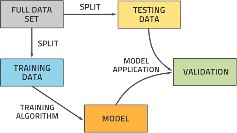
In training any model, we use empirical data to tune the model parameters such that the model fits best to the data. That data is called the training data. Having made the model, we want to know how good the model is. While it is interesting how well it performs on the training data, this is not the final answer. We are usually much more concerned by how the model will perform on data it has not seen during its own construction, the testing data.
Some training algorithms not only the training data to tune the model parameters but, additionally, use a dataset to determine when the training should stop because no significant model performance improvement can be expected. It is common to use the testing data for this purpose. It then may become necessary to generate a third dataset, the validation data, for testing the model on data that was not used at all during training.
It is common practice therefore to split the original dataset into two parts. We generally use 70%–85% of the data for training and the remainder for testing. Fig. 3.15 illustrates this process.
Figure 3.15The full dataset must be split into data to be used for model training and data to be used for testing the model's performance.
The choice of which data goes into the training or testing datasets needs to be made carefully because both datasets should be representative and significant for the problem at hand. Often, these are chosen randomly, and so chances are that some unintended bias enters the choice. This gave birth to the idea of cross-validation, which is the current accepted standard for demonstrating a model's performance.
The original dataset is divided into several, roughly equally sized, parts. It is typical to use 5 or 10 such parts and they are called folds. Let's say that we are using folds. We now construct different training datasets and different testing datasets. The testing datasets consists of one of the folds and the training datasets consist of the rest of the data. Fig. 3.16 illustrates this division.
Figure 3.16An illustration of how to divide the full dataset into folds for cross-validation.
We now go through distinct trainings, resulting in distinct models. Each model is tested using its own testing dataset. The performance is now estimated to be the average performance over all the trained models. Generally, only the best model is kept but its performance has been estimated in this averaged fashion. This way of assessing the performance is more independent of the dataset bias than assessing it using any one choice of testing dataset and so it is the expected performance estimation method.
Having done all this, we could get the idea that we could use all models, evaluate them all in each real case and take the average of them all to be the final output of an overarching model. This is a legitimate idea that is called an ensemble model. The ensemble model consists of several fully independent models that may or may not have different architectures and that are averaged to yield the output of the full model. These methods are known to perform better on many tasks as compared to individual models, at least in the sense of variance. However, it comes at the expense of resources as several models must not only be trained but maintained and executed in each case. Especially for industrial applications, that often require real-time model execution, this may be prohibitive.
It is important to mention that the model and the training algorithm usually have some fixed parameters that a data scientist must choose prior to training. An example is the number of layers of a neural network and the number of neurons in each layer. Such parameters are called hyperparameters. It is rare indeed that we know what values will work best in advance. In order to achieve the best overall result, we must perform hyperparameter tuning. Often this is done in a haphazard trial-and-error method by hand because we do not want to try too many combinations. After all, we should ideally perform the full cross-validation for each choice and each one of those involves several model trainings. All this training takes time. It is possible however to perform automated hyperparameter tuning by using an optimization algorithm. If model performance is very important and we have both time and resources to spare, hyperparameter tuning is a very good way to improve model performance. Once this has been exhausted, there is little more one can do.
3.5. How good is my model?
On a weekly basis, we read of some new record of accuracy of some algorithm in a machine learning task. Sometimes it's image classification, then it's regression, or a recommendation engine. The difference in accuracy of the best model or algorithm to date from its predecessor is shrinking with every new advance.
A decade ago, accuracies of 80% and more were already considered good on many problems. Nowadays, we are used to seeing 95% already in the early days of a project. Getting (1) more sophisticated algorithms, (2) performing laborious hyperparameter tuning, (3) making models far more complex, (4) having access to vastly larger data sets, and last—but certainly not least—(5) making use of incomparably larger computer resources has driven accuracies to 99.9% and thereabouts for many problems.
Instinctively, we feel that greater accuracy is better and all else should be subjected to this overriding goal. This is not so. While there are a few tasks for which a change in the second decimal place in accuracy might actually matter, for most tasks this improvement will be irrelevant—especially given that this improvement usually comes at a heavy cost in at least one of the above five dimensions of effort.
Furthermore, many of the very sophisticated models that achieve extremely high accuracies are quite brittle and thus vulnerable to unexpected data inputs. These data inputs may be rare or forbidden in the clean data sets used to produce the model, but strange inputs do occur in real life all the time. The ability for a model to produce a reasonable output even for unusual inputs is its robustness or graceful degradation. Simpler models are usually more robust and models that want to survive the real world must be robust.
A real-life task of machine learning sits in between two great sources of uncertainty: Life and the user. The data from life is inaccurate and incomplete. This source of uncertainty is usually so great that a model accuracy difference of tens of a percent may not even be measurable in a meaningful way. The user who sees the result of the model makes some decision on its basis and we know from a large body of human-computer-interaction research that the user cares much more about how the result is presented, than the result itself. The usability of the interface, the beauty of the graphics, the ease of understanding and interpretability count more than the sheer numerical value on the screen.
In most use cases, the human user will not be able to distinguish a model accuracy of 95% from 99%. Both models will be considered “good” meaning that they “solve” the underlying problem that the model is supposed to solve. The extra 4% in accuracy are never seen but might have to be bought by many more resources both initially in the model-building phase as well as in the on-going model execution phase. This is the reason we see so many prize-winning algorithms from competitions never being used in a practical application. They have high accuracy but either this high accuracy does not matter in practice or it is too expensive (complexity, project duration, financial cost, execution time, computing resources, etc.) in real operations.
We must not compare models based on the simplistic criterion of accuracy alone but measure them in several dimensions. We will then achieve a balanced understanding of what is “good enough” for the practical purpose of the underlying task. The outcome in many practical projects is that we are done much faster and with less resources. Machine learning should not be perfectionism but pragmatism.
3.6. Role of domain knowledge
Data science aims to take data from some domain and come to a high-level description or model of this data for practical use in solving some challenge in that domain. How much knowledge about the domain does the data scientist have to have to do a good job?
Before starting on a data science project, someone must define (1) the precise domain to focus on, (2) the particular challenge to be solved, (3) the data to be used, and (4) the manner in which the answer must be delivered to the beneficiary. All four of these aspects are not data science in themselves but have significant impact on both the data science and the usefulness of the entire effort. Let's call these aspects the framework of the project.
While doing the data science, the data must be assessed for its quality: precision, accuracy, representativeness, and significance.
• Precision: How much uncertainty is in a value?
• Accuracy: How much deviation from reality is there?
• Representativeness: Does the dataset reflect all relevant aspects of the domain?
• Significance: Does the dataset reflect every important behavior/dynamic in the domain?
In seeking a high-level description of the data, be it as a formulaic model or some other form, it is practically expedient to be guided by existing descriptions that may only exist in textual, experiential, or social forms, that is, in forms inaccessible to structured analysis. In real projects we find that data science often finds (only) conclusions that are trivial to domain experts or does not find a significant conclusion at all. Incorporating existing descriptions will prevent the first and make the second apparent a lot earlier in the process.
It thus becomes obvious that domain knowledge is important both in the framework as well as the body of a data science project. It will make the project faster, cheaper, and more likely to yield a useful answer.
This situation is beautifully illustrated by the famous elephant parable. Several blind persons, who have never encountered an elephant before, are asked to touch one and describe it. The descriptions are all good descriptions, given the experience of each person, but they are all far from the actual truth, because each person was missing other important data, see Fig. 3.17.
Figure 3.17The parable of the six blind people trying to describe an elephant by touching part of it.
This problem could have been avoided with more data or with some contextual information derived from existing elephantine descriptions. Moreover, the effort might be better guided if it is clear what the description will be used for.
A domain expert typically became an expert by both education and experience in that domain. Both imply a significant amount of time spent in the domain. As most domains in the commercial world are not freely accessible to the public, this usually entails a professional career in the domain. This is a person who could define the framework for a data science project, as they would know what the current challenges are and how they must be answered to be practically useful, given the state of the domain as it is today. The expert can judge what data is available and how good it is. The expert can use and apply the deliverables of a data science project in the real world. Most importantly, this person can communicate with the intended users of the project's outcome. This is crucial, as many projects end up being shelved because the conclusions are either not actionable or not acted upon.
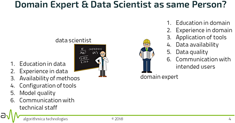
A data scientist is an expert in the analysis of data. Becoming such an expert also requires a significant amount of time spent being educated and gaining experience. Additionally, the field of data science is developing rapidly, so a data scientist must spend considerable time keeping up with innovations. This person decides which of the many available analysis methods should be used in this project and how these methods are to be parametrized. The tools of the trade (usually software) are familiar to this person, and he or she can use them effectively. Model quality and goodness-of-fit are evaluated by the data scientist. Communication with technical persons, such as mathematicians, computer scientists, and software developers, can be handled by the data scientist (Fig. 3.18).
Figure 3.18The difference in roles between a data scientist and a domain expert.
The expectation that a single individual would be capable of both roles is unrealistic, in most practical cases. Just the requirement of time spent, both in the past as well as regular upkeep of competence, prohibits dual expertise. In some areas it might be possible for a data scientist to learn enough about the domain to make a good model, but assistance would still be needed in defining the challenge and communicating with users, both of which are highly non-trivial. It may also be possible for a domain expert to learn enough data science to make a reasonable model, but probably only when standardized tools are good enough for the job (Fig. 3.19).
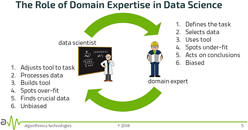
Figure 3.19A project is much more likely to succeed if a domain expert and data scientist collaborate.
If there are two individuals, they can get excellent results quickly by good communication. While the domain expert (DE) defines the problem, the data scientist (DS) chooses and configures the right toolset to solve it. The representative, significant, and available data are chosen by the DE and processed by the DS. The DS builds the tool (that might involve programming) for the task given the data, and the DE uses the tool to address the challenge. Having obtained a model, the DS can spot over-fitting, where the model has too many parameters so that it effectively memorizes the data, leading to excellent reproduction of training data, but poor ability to generalize. The DE can spot under-fitting, where the model provides too little accuracy or precision to be useful or applied in the real world. The DS can isolate the crucial data in the dataset needed to make a good model; frequently this is a small subset of all the available data. The DE then acts on the conclusions by communicating with the users of the project and makes appropriate changes. The DS approaches the project in an unbiased way, looking at data just as data. The DE approaches the project with substantial bias, as the data has significant meaning to the DE, who has pre-formed hypotheses about what the model should look like. It is important to note that bias, in this context, is not necessarily a detriment to the effort.
It is instructive to think what the outcome can be if we combine a certain amount of domain knowledge with a certain level of data science capability. The vision below is the author's personal opinion but is probably a reasonable reflection of what is possible today.
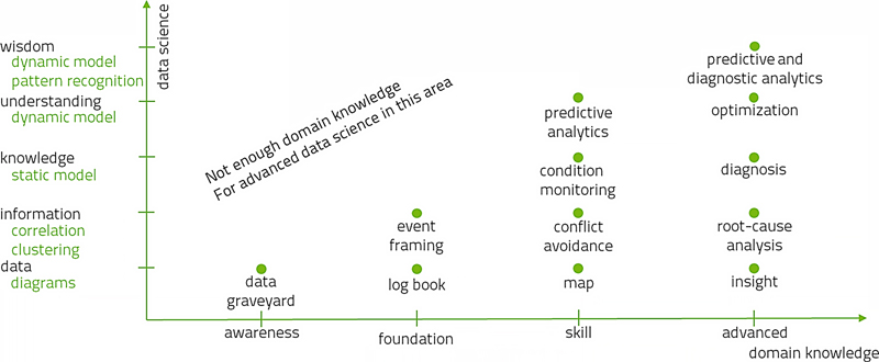
First, for the sake of this discussion, let's divide domain knowledge into four levels: (1) Awareness is the basic level where we are aware of the nature of the domain. (2) Foundation is knowing what the elements in the domain do, equivalent to a theoretical education. (3) Skill is having practical experience in the domain. (4) Advanced is the level where there is little left to learn and where skill and knowledge can be provided to other people, that is, this person is a domain expert.
Similarly, we can divide up data science into five levels: (1) Data is where we have a table or database of numbers. We can do little more than draw diagrams with this. (2) Information is where we have descriptive statistics about the available data, such as correlations and clusters. (3) Knowledge is when we have some static models. (4) Understanding is when we have dynamic models. The distinction between static and dynamic models is whether the model incorporates the all-important variable of time. A static model makes a statement about how one part of the process affects another, whereas a dynamic model makes additional statements about how the past affects the future. (5) Wisdom is when we have both dynamic models and pattern recognition, for now we can tell what will happen when.
In Fig. 3.20 are several technologies that exist today ordered by the level of data science that they represent and the amount of domain knowledge that was necessary to create them. There are no technologies in the upper left of the diagram because one cannot make such advanced data science with so little domain knowledge.
Figure 3.20More is possible if sophisticated domain knowledge is combined with deep data science expertise.
In conclusion, data science needs domain knowledge. As it is unreasonable to expect any one person to fulfill both roles, we are necessarily looking at a team effort.
3.7. Optimization using a model
We train a machine learning model by adjusting its parameters such that its performance—the least-squares difference between model output and expected output—is a minimum. Such a task is called optimization and methods that do this are called optimization algorithms. Every training algorithm for a model is an example of an optimization algorithm. Usually these algorithms are highly customized to the kind of machine learning model that they deal with. We will not treat these methods as that level of detail is beyond the scope of the book.
There are also some general-purpose optimization algorithms that work on any model. These methods can be used on the machine learning model that was just made. If we have a model for the efficiency of a gas turbine, for example, as a function of a multitude of input variables, then we can ask: How should the input variables be modified in order to achieve the maximum possible efficiency? This is a question of process optimization or advanced process control, which is also sometimes—strangely—called statistical process control (Coughanowr, 1991; Qin and Badgwell, 2003).
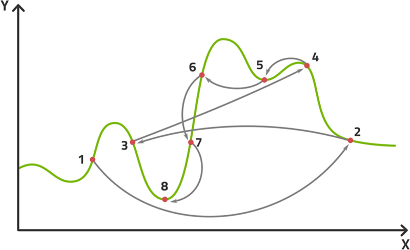
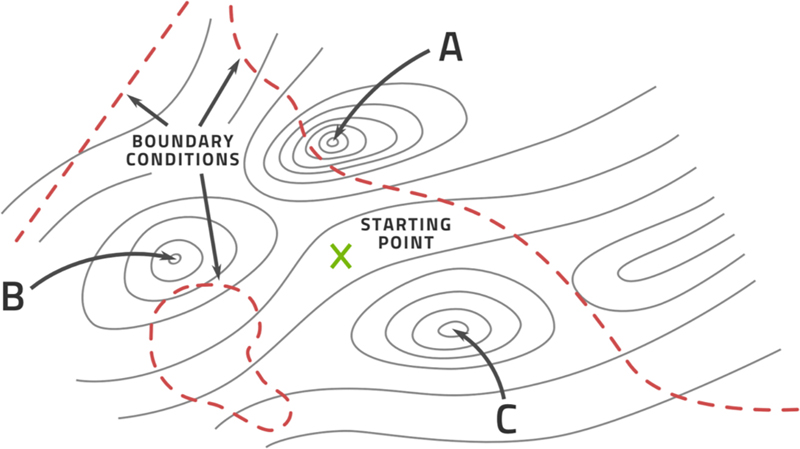
For the sake of illustration, let's say that we have only two manipulated variables that we can change in order to affect the efficiency. Fig. 3.21 is a contour plot that illustrates the situation. The horizontal and vertical directions are the two manipulated variables. The efficiency resulting from these is displayed in contour lines just like on a topographical map. The points labeled A, B, and C are the peaks in the efficiency.
Figure 3.21A contour plot for a controlled variable like efficiency in terms of two manipulated variables.
Any practical problem has boundary conditions, that is, conditions that prevent us from a particular combination of manipulated variables. These usually arise from safety concerns, physical constraints, or engineering limitations and are indicated by the dashed lines. The peak labeled A for instance is not allowed due the boundary conditions.
The starting point in the map is the current combination of manipulated variables. Whatever we do is a change away from this point. What is the best point? It is clearly either B or C. The resolution of the map does not tell us but in practice these two efficiencies may be quite close to one another. This is like a car's GSP choosing one route over another because it computes one path to be a few seconds shorter. Whichever point we choose to head for, the next task is to find the right path. In terms of efficiency this is perpendicular to the contour lines, that is, the steepest ascent.
Computing these actions in advance, with the appropriate amount of time that is needed in between variable changes, is the purpose of the optimization. Then the actions can be realized in the physical process and the efficiency should rise as a result.
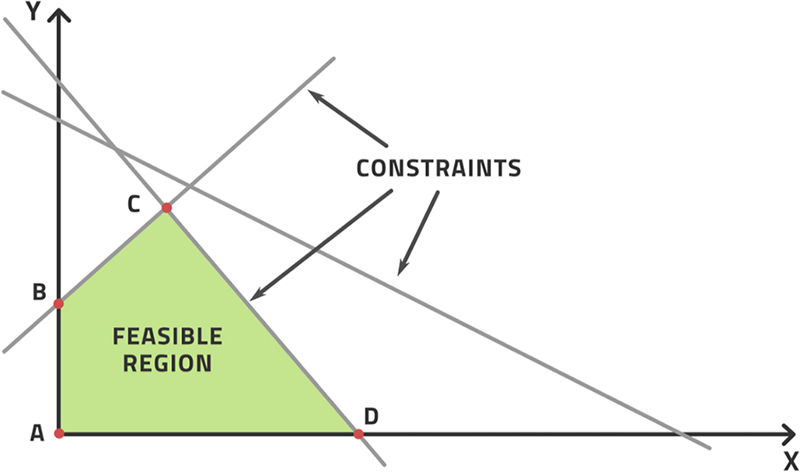
There is a special case of optimization where the objective is a linear function of all the measurable variables. This is known as linear programming and is displayed in Fig. 3.22. The boundary conditions, or constraints, define a region that contains all the points allowed. We can prove that the best solution is on the boundary of the region and solving such problems is relatively simple and fast. Linear optimization problems are routinely solved in the oil and gas industry, particularly in financial optimization, for example, how much of each refinery end product to make during any one week in a refinery.
Figure 3.22Linear optimization illustrated as a region bounded by constraints with the optimal points necessarily on the border.
So, we have a model where the function is potentially a highly complex machine learning model, is potentially a long vector of various measurements, and is the target of the optimization, that is, the quantity that we want to maximize. Of the elements of , there will be some that the operators of the facility can change at will. These are called set-points because we can set them. There will also be values that are fixed by powers that are completely beyond our control, for example, the weather, market prices, raw material qualities and other factors determined outside our facility. These are fixed by the outside world and so correspond to constraints.
Now we can ask: What are the values of the set-points, given all the boundary conditions and constrained values, that lead to the largest possible value of ? This is the central question of optimization. Let us call any setting of the set-points that satisfies all boundary conditions, a solution to the problem. We then seek the solution with the maximum outcome in .
One of the most general ways of answering this question is the method of simulated annealing. This method starts from the current setting of the set-points. We then consider a random change in the vector of set-points such that this second point is still a solution. If the new point is better than the old, we accept the change. If it is worse, we accept it with a probability that starts off being high and that gradually decreases over the course of the iterations. We keep on making random changes and going through this probabilistic acceptance scheme. Once the value of the optimization target does not change anymore over some number of iterations, we stop the process and choose the best point encountered over the entire journey. See Fig. 3.23 for an illustration of a possible sequence of points in search for the global minimum.
Figure 3.23Simulated annealing illustrated as a sequence of jumps, sometimes for the better and sometimes for the worse, eventually converging on the global minimum.
This method provably converges to the best possible point (the global optimum). Even if we cut off the method after a certain finite amount of resources (such as computation time or number of transitions) has been spent on it, we can rely on the method having produced a reasonable improvement relative to the resources spent.
There are a few fine points of simulated annealing and there is much discussion in the literature on how to calculate the probability of accepting a temporary change for the worse, how to judge if the method has converged, how to generate the new trial point and so on (Bangert, 2012).
3.8. Practical advice
If you want to perform a machine learning project in real-life, here is some advice on how to proceed.
First, all the steps outlined in Section 2.10 should be followed so that you have a clean, representative, significant dataset and you are clear on what you want as the final outcome and how measure whether it is good enough for the practical purpose.
Second, as mentioned in Section 3.6 it is a good idea to conduct such a project with more than one person. Without going into too much detail here, you may need a small team consisting of one or several of these persons: an equipment operator, a maintenance engineer, a process engineer, a process control specialist, a person from the information technology (IT) department, a sponsor from higher management, a data scientist, and a machine learner. From practical experience, it is virtually impossible to do such a project by oneself.
Third, select the right kind of mathematical modeling approach to solve your problem. Several popular ones were outlined earlier. There are more but these represent most models applied in practice. You may ask yourself the following questions:
1. Do you need to calculate values at a future time? You will probably get the best results from a recurrent neural network such as an LSTM as it is designed to model time dependencies.
2. Do you need to calculate a continuous number in terms of others? This is the standard regression problem and can be reliably solved using deep neural networks.
3. Do you need to identify the category that something belongs to? This is classification and the best general classification method is random forest.
4. Do you need to compute the likelihood that something will happen (risk analysis) or has happened (root-cause analysis)? Bayesian networks will do this very nicely.
5. Do you need to do several of these things? Then you will need to make more than one model.
Fourth, every model type and training method has settings. These are the hyperparameters as the model coefficients are usually called the parameters. Having selected the model type, you will now have to set the hyperparameters. This can be done by throwing resources at the issue and doing an automated hyperparameter tuning in which a computer tries out many of them and selects the best. If you have the time to do this, do it. If not, you will need to think the choices through carefully. The main consideration is the bias-variance-complexity trade-off that mainly concerns those hyperparameters that influence how many parameters the model has.
Fifth, perform cross-validation as described in Section 3.4 to calculate all the performance metrics you have chosen correctly. This will get you an objective assessment of how good your model is as described in Section 3.5.
Sixth, if your goal was the model itself, then you now have it. However, if your goal is to derive some action from the model, you now need to compute that action using the model and this usually requires an optimization algorithm as described in Section 3.7. Several such are available but simulated annealing has several good properties that make it an ideal candidate for practical purposes.
Seventh, communicate your results to the rest of the team and to the wider audience in a way that they can understand it. You may need the domain experts to help you do this properly. This audience may need to change their long-established ways based on your results, and they may not wish to do so. The implied change management in this communication is the most difficult challenge of the entire project. In my personal experience this is the cause of failure in almost all failed data science projects in the industry, which is why we will address this at length in other chapters of this book.

 and
and  whereas unsupervised learning consists of examples like
  and
and  . It is clear from this difference that we can expect supervised methods to be much more accurate in reproducing the outcome. Unsupervised methods are expected to learn the structure of the input data and recognize some patterns in them.
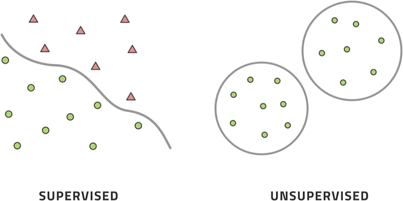
 , has no meaning, that is, the difference between the two datapoints does not necessarily belong to group 1 nor does group membership necessarily even make sense for the difference.
 and the difference is 1 ton per hour of flow, which is a meaningful quantity that we can understand.
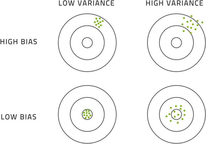
 enters the network. This is called the input layer and has several neurons equal to the number of elements in the input vector. On the right side, the output vector
  exits from the network. This is called the output layer and has several neurons equal to the number of elements in the output vector; this is the result of the calculation. In between them are several hidden layers. The number of hidden layers and the number of neurons in each are up to us to choose and is referred to as the topology of the neural network.
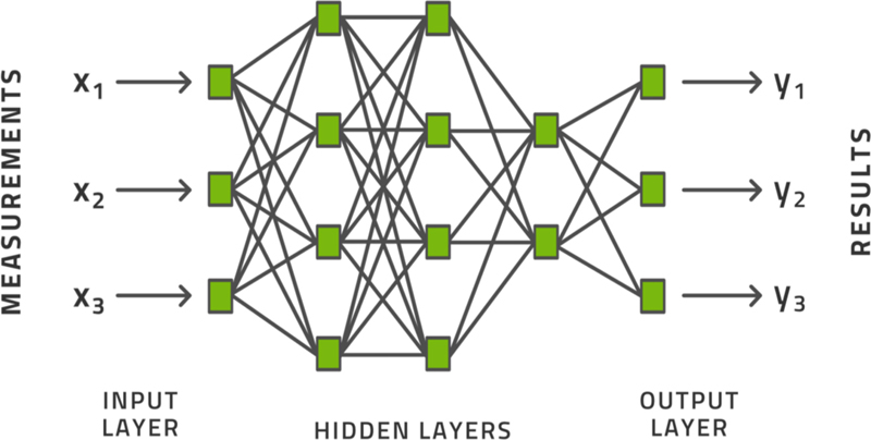

 is not learnt but decided on beforehand. Considerable research has been put into this choice. While older literature prefers
  , we now have evidence that
  performs significantly better in virtually all tasks for all layers except the outermost for which we usually choose the identity function. They are both displayed in Fig. 3.8.
 and vectors
  , the neural network becomes a specific model. The main reason it is so famous is that it has the property of universal approximation. This property states that the formula can represent any continuous function with arbitrary accuracy. There are other formulae that have this property, but neural networks were the first ones that were practically used with this feature in mind. In practice, this means that a neural network can represent your data. What the property does not do is tell us how many layers and how many neurons per layer to choose. It also does not tell us how to find the correct parameter values so that the formula does in fact represent the data. All we know is that the neural network can represent the data.
 are independent of each other. For example, if we take a manual fluid sample from a well once per day and perform a laboratory analysis on it, we can assume that today's observation is largely independent of yesterday's observation but may well depend on the pressure and temperature right now. In this context, we may use pressure and temperature as inputs and expect the neural network to represent the laboratory measurement.
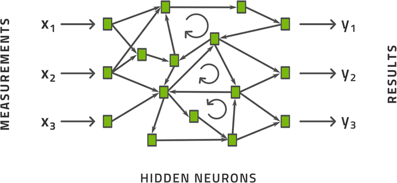

 and
and  are the weight and bias parameters of the LSTM cell. All weights and biases of the entire network must be tuned by the learning algorithm. The evolution of the internal state of the network
  is the memory of the network that can encapsulate the time dynamics of the data.
 for many successive values of time
  . The model outputs the same time-series but at a later time
  , where
  is the forecast horizon. This is the essence of how LSTM can forecast a time-series,


 folds. We now construct
  different training datasets and
  different testing datasets. The testing datasets consists of one of the folds and the training datasets consist of the rest of the data. Fig. 3.16 illustrates this division.
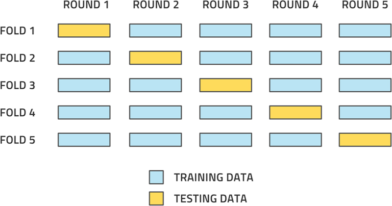
 distinct trainings, resulting in
  distinct models. Each model is tested using its own testing dataset. The performance is now estimated to be the average performance over all the trained models. Generally, only the best model is kept but its performance has been estimated in this averaged fashion. This way of assessing the performance is more independent of the dataset bias than assessing it using any one choice of testing dataset and so it is the expected performance estimation method.
 models, evaluate them all in each real case and take the average of them all to be the final output of an overarching model. This is a legitimate idea that is called an ensemble model. The ensemble model consists of several fully independent models that may or may not have different architectures and that are averaged to yield the output of the full model. These methods are known to perform better on many tasks as compared to individual models, at least in the sense of variance. However, it comes at the expense of resources as several models must not only be trained but maintained and executed in each case. Especially for industrial applications, that often require real-time model execution, this may be prohibitive.
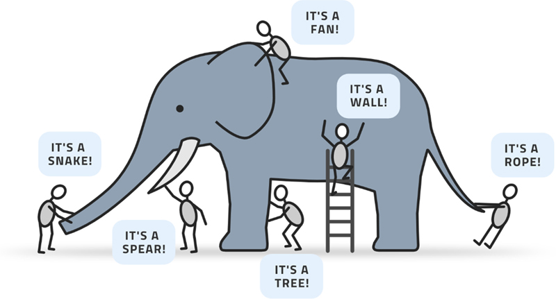
 where the function
  is potentially a highly complex machine learning model,
  is potentially a long vector of various measurements, and
  is the target of the optimization, that is, the quantity that we want to maximize. Of the elements of
  , there will be some that the operators of the facility can change at will. These are called set-points because we can set them. There will also be values that are fixed by powers that are completely beyond our control, for example, the weather, market prices, raw material qualities and other factors determined outside our facility. These are fixed by the outside world and so correspond to constraints.
 ? This is the central question of optimization. Let us call any setting of the set-points that satisfies all boundary conditions, a solution to the problem. We then seek the solution with the maximum outcome in
  .
.