
Chapter 11: Detecting Electric Submersible Pump Failures
Long Peng
Guoqing Han
Arnold Landjobo Pagou
Jin Shu China University of Petroleum, Beijing, China
Abstract
Electric Submersible Pumps (ESP) are currently widely employed to help enhance production for nonlinear-flowing wells with high production and high water cut. A broken shaft is common in the oil industry, which leads to production disruptions, resulting in significant economic losses. The objective of this chapter is to evaluate Principal Component Analysis (PCA) as an unsupervised machine learning technique to detect the cause of the breakage of the ESP shaft. This method was successfully applied in the Penglai block of the Bohai Oilfield in China to detect the ESP shaft fracture in real-time. A two-dimensional plot of the first two principal components can be used to identify different clusters in the stable region, unstable region, and failure region. In this way, potential ESP shaft fractures will be found when the cluster starts deviating away from the stable region. Moreover, a PCA diagnostic model is built to forecast the time at which the ESP shaft fracture will occur and to determine the main decision variable most responsible for the event. This paper demonstrates that the application of the PCA method performs well in monitoring the ESP system and forecasts the impending breakage of an ESP shaft with high accuracy.
Keywords
electric submersible pump
principal component analysis
broken shaft
fault diagnosis
PCA diagnostic model
unsupervised machine learning
predictive maintenance
11.1. Introduction
Electric Submersible Pumps are currently widely employed to help enhance the production for nonlinear flowing well with high production, high water cut, and offshore oil wells due to its simple structure and high efficiency (Ratcliff, Gomez, Cetkovic, & Madogwe, 2013). Among all the oil artificial lift systems, ESP is preferred because it can produce high volumes in higher temperatures and reach deeper depths. However, it is often observed that the ESP system reaches the point of service interruption. The breakage of the pump shaft is a severe issue for the operating company as it generates an estimated loss of hundreds of millions of oil barrels. Should the pump shaft break, the motor current would drop suddenly, and the production would be interrupted. The reason of the pump shaft breakage is bad pump assembly or pump aging.
The development of sensors and data acquisition systems make it possible for ESP systems to continuously record the intake pressure, intake temperature, pump head, discharge pressure, discharge temperature, motor temperature, motor current, leakage current, vibration and so on. Those data would be recorded at regular intervals and transmitted to surface Remote Terminal Units (RTUs) (Bates et al., 2004). For those broken shaft wells, statistics, or machine learning algorithms can be used for failure analysis and health monitoring.
The objective of this paper is to evaluate principal component analysis (PCA) as a monitoring tool to forecast the breakage of the ESP shaft.
11.2. ESP data analytics
ESP operation system has developed over the years and is considered as an effective means to lift crude oil under wellbore conditions. There is increased attention on ESP systems due to the fast development of ESP sensors in the oil industry. The ESP sensors gather a vast amount of data, including dynamic data, static data, and historical data (Abdelaziz, Lastra, & Xiao, 2017), as shown in Fig. 11.1. In the past few years, wells using ESP technology have been tracked by physical well site visits, which require enormous human resources to make necessary adjustments to the well operating system. The oil and gas industry has begun applicating data analytic to improve production efficiency (Stone et al., 2007; Takacs, 2017) proposed the ammeter charts as the primary diagnostic method to monitor ESP performance.

Figure 11.1 ESP data are available.
Furthermore, the emergence of the Supervisory Control and Data Acquisition (SCADA) system has provided convenience for field personnel to monitor and control the ESP well behavior (Ratcliff et al., 2013). The SCADA system can achieve the full realization of continuously recording ESP production data in real-time.
In recent years, “Big Data” collected on ESP sensors is framing the key point of how to extract the most essential information to evaluate the ESP operating system. Data-driven models coupled with machine learning, have been used to judge and optimize well production. Bravo, Rodriguez, Saputelli, & Rivas Echevarria (2014) described data analytic as an integral process of collecting and analyzing big data.
Pump shaft fracture is a common fault in the ESP operating system. Based on operation data acquired by ESP ground and downhole sensors, data-driven model analytics will play an important role in monitoring the breakage of the pump shaft. There is a need to evolve from a supervised method toward fault diagnosis to an approach according to data-driven models for predictive maintenance. PCA is widely considered as a pre-processing method for dimensionality reduction, eigenvalue extraction and data visualization (Abdelaziz et al., 2017). PCA can be used as an unsupervised machine learning technique to analyze the reason of the pump shaft breakage.
11.3. Principal Component Analysis
Jackson (2005) defines PCA as an unsupervised dimensionality reduction means, which transfers data linearly and creates a new set of parameters called “principal component”. What is known to us is that ESP data are generally highly correlated; i.e. an increase of the wellhead pressure will lead to an increase of intake and discharge pressure, which will finally cause an increase of the motor temperature. PCA makes use of the interdependence of original data to build a PCA model. This results in the reduction of the production parameters’ dimension by taking advantage of the linear combinations and by creating a new Principal Component space (PCs). This PCs can evaluate the ESP system only by several principal components, making the process much easier.
For those wells with pump shaft fracture, a PCA model can be established to analyze a few months of production data before the pump breaks. Once the robust PCA model is built, the cause of the breakage of the pump shaft will be monitored and diagnosed. The basic PCA model can be represented as follows:
 (11.1)
where  is the input matrix (
 ); it represents original parameters;
  is the loading matrix (
 ); it represents the contribution of original parameters;
  is the score matrix (
 ); it represents the relationship between original parameters;
  is the residual matrix (
 ); it represents the uncaptured variance;
  is the number of time steps (Gupta, Saputelli, & Nikolaou, 2016);
  is the number of original parameters;
  is the number of principal components.
is the input matrix (); it represents original parameters; is the loading matrix (); it represents the contribution of original parameters; is the score matrix (); it represents the relationship between original parameters; is the residual matrix (); it represents the uncaptured variance; is the number of time steps (Gupta, Saputelli, & Nikolaou, 2016); is the number of original parameters; is the number of principal components.The first principal component contains the highest variance, implying that the first principal component contains the most information. The second principal component will capture the next highest variance, which has already removed the information of the first principal component. By this means, the third, fourth, …,  th principal component can be constructed to evaluate the original system. Fig. 11.2 summarizes the comments above.
th principal component can be constructed to evaluate the original system. Fig. 11.2 summarizes the comments above.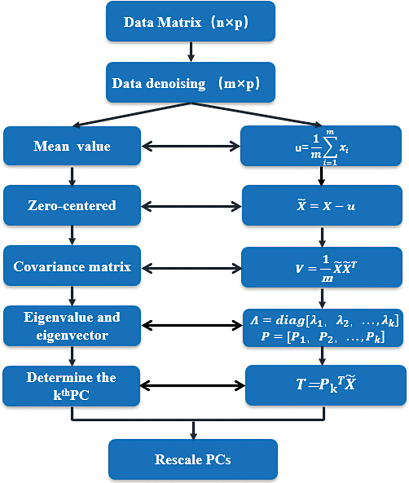
Figure 11.2 The architecture of PCA.
As is often the case, the PCA model finds  principal component to construct the PCs, which retains most of the information that belongs to the initial system. The
  th principal component is denoted in the following equation taking PC1 as an example.
principal component to construct the PCs, which retains most of the information that belongs to the initial system. The th principal component is denoted in the following equation taking PC1 as an example. (11.2)
When working with two dimensions, Ionita and Schiopu (2010) depicted this case using Fig. 11.3. PCA is used to find patterns in high-dimensional data and to transform the stable region data, which is usually characterized as a tight cluster or cloud data sets. In this way, anomalies in the ESP operation system will be detected by establishing a PCA model with a normal production dataset. The first two PCs have the highest variance, explaining most of the information in the original parameters visualized only by the first two PCs.
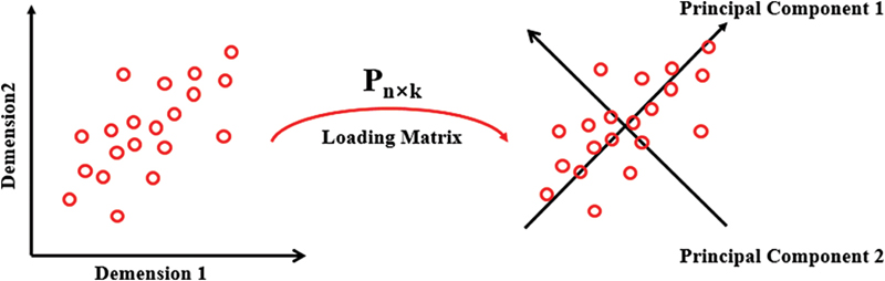
Figure 11.3 The geometric meaning of PCA with two dimensions.
11.4. PCA diagnostic model
PCA diagnostic model is applied to identify the cause and the time of pump shaft fracture. The Hotelling Tsquare statistic ( ) and Squared Prediction Error (SPE) are used to numerically visualize scalar statistics (Yue and Qin, 2001).
  is a univariate statistic that plays an important role in multivariate hypothesis testing, SPE is frequently used in multivariate statistical process control.
  and SPE are applied to analyzing whether the decision variable is satisfactory with the requirement of stable running. With this method, the contribution of each decision variable towards failure can be determined. The failure issue will ultimately be diagnosed due to the ranking of the contribution of each of the decision variables. The potential anomalies are related to the correlative higher ranking or highest decision variables.
) and Squared Prediction Error (SPE) are used to numerically visualize scalar statistics (Yue and Qin, 2001). is a univariate statistic that plays an important role in multivariate hypothesis testing, SPE is frequently used in multivariate statistical process control. and SPE are applied to analyzing whether the decision variable is satisfactory with the requirement of stable running. With this method, the contribution of each decision variable towards failure can be determined. The failure issue will ultimately be diagnosed due to the ranking of the contribution of each of the decision variables. The potential anomalies are related to the correlative higher ranking or highest decision variables.
 (11.3)
 (11.4)
where  is the
  th timestep of the input matrix;
  is the inverse of the covariance matrix (Westerhuis, Gurden, & Smilde, 2000);
  is the eigenvectors of the covariance matrix;
  is the residual loading matrix;
  is the identity matrix;
is the th timestep of the input matrix; is the inverse of the covariance matrix (Westerhuis, Gurden, & Smilde, 2000); is the eigenvectors of the covariance matrix; is the residual loading matrix; is the identity matrix; (11.5)
 (11.6)
where  and
and  donate the confidence limits for
  and SPE.
  follows an F-distribution, the F-distribution is a right-skewed distribution for studying population variances. Where
  represents the boundary that the Cumulative Distribution Function of the possible distribution is 0.99. Once it exceeds the control limit
  ,
,  is regarded as a potential anomaly. According to Jackson and Mudholkar (1979), SPE follows a Gaussian distribution, Gaussian distribution is symmetric about the mean, showing that data near the mean are more frequent in occurrence than data far from the mean. Where
  represents the boundary and
  is equal to 0.99. SPE is considered abnormal when it exceeds the control limit
  .
.
and donate the confidence limits for and SPE. follows an F-distribution, the F-distribution is a right-skewed distribution for studying population variances. Where represents the boundary that the Cumulative Distribution Function of the possible distribution is 0.99. Once it exceeds the control limit , is regarded as a potential anomaly. According to Jackson and Mudholkar (1979), SPE follows a Gaussian distribution, Gaussian distribution is symmetric about the mean, showing that data near the mean are more frequent in occurrence than data far from the mean. Where represents the boundary and is equal to 0.99. SPE is considered abnormal when it exceeds the control limit .Cho, Lee, Choi, Lee, & Lee (2005) proposed the following equation defining the contribution of each decision variable  based on
  and SPE
based on and SPE (11.7)
 (11.8)
where  represents the
  column of identity matrix
  . The higher the contribution of each decision variable, the greater the possibility of potential anomalies.
represents the column of identity matrix . The higher the contribution of each decision variable, the greater the possibility of potential anomalies.11.5. Case study: diagnosis of the ESP broken shaft
11.5.1. Selection of the ESP broken shaft variables
Production data of ten ESP wells with broken shaft are recorded at a frequency of 20 minutes by ESP downhole and ground sensors. The ESP downhole and ground sensors start to collect the production data since ten ESP wells are put into production and come to an end when the breakage of the pump shaft occurs in these wells. These ESP broken shaft wells, including E52ST1, C06ST1, B50ST2, E20ST2, A11ST1, B03ST1, B48ST1, E21ST1, E47ST1, and E42ST1 are from the Penglai block of Bohai Oilfield in China. Two different types of datasets are collected. They include:
- • Data records containing input variable parameters of casing choke, casing line pressure, casing pressure, casing gas rate, ESP intake pressure, ESP discharge pressure, flowline pressure, flowline temperature, intake temperature, motor current, motor leak current, motor power, motor temperature, motor torque current, motor vibration, motor voltage, tubing choke, and VFD frequency.
- • Data records containing information on the time when the breakage of the pump shaft occurs in each well.
11.5.2. Score of principle components
A PCA model is constructed based on the input variables obtained. Different principal components are ranked according to the decreasing order of variance captured. Taking well E52ST1, for example, it is observed that eight principal components capture more than 99% of the variance of the original input parameters, as shown in Fig. 11.4.

Figure 11.4 The captured variance of well E52ST1 by Principal Components.
The first two principal components have the highest variance and capture probably 70% variance in the original data. A two-dimensional plot of scores of Principal Component 1 and Principal Component 2 is used to observe different clusters during the stable, unstable or failure periods. The ESP operates normally, and all the input variable parameters are in normal working range during the stable periods. When it comes to the unstable periods, some of the input variable parameters are obviously abnormal, but the ESP is still operating. Furthermore, the breakage of the pump shaft occurs, and the ESP breaks down during the failure periods.
Fig. 11.5 represents the score plot of Principal Component 1 and Principal Component 2 of the historical data from well E52ST1 with pump shaft fracture. During this time frame, as the time step increases, the result clearly shows three different clusters for the stable region, unstable region and failure region. In the beginning, the ESP is put into production. It is observed that the normal operating input variable parameters form a stable region cluster. After working long hours, some of the input variable parameters start to deviate from the normal working range, but the ESP is still operating. When this abnormal behavior takes place, an unstable region deviating away from the stable region will form. The ESP continues to work for a period of unstable time. Finally, the breakage of the pump shaft occurs, and the ESP breaks down. From the plot below, we can observe that the black failure region is far away from the stable region. This two-dimensional plot of scores of Principal Component 1 and Principal Component 2 can be of great significance to monitor ESP performance in real-time against the previously normal operating zone to forewarn field engineers of potential failure if the cluster starts deviating away from the stable region.

Figure 11.5 Well E52ST1 scores plot of Principal Component 1 and Principal Component 2.
11.5.3. Pump broken shaft identification
Production data from the stable region is normalized and used as the input matrix (Xtraining) to construct the robust PCA model. Besides, historical data corresponding to an unstable or a failure region period is selected as a testing dataset (Xtesting) fed to the PCA model. This process can be repeated for the historical broken shaft events leading to a failure. Also, the PCA diagnostic model is built to predict the time at which the breakage of the pump shaft occurs, and to determine the decision variable most responsible for the pump shaft fracture.
The contribution of each of the decision variables can be calculated by the PCA diagnostic model based on Eqs. (11.7) and (11.8). The decision variables with higher ranking or highest contribution are more related to the pump shaft fracture. The decision variables are ranked based on their contribution. Taking well E52ST1 as an example, it is shown in Fig. 11.6 that the motor torque current has the highest contribution for the failure region. Therefore, this kind of contribution chart can be used to diagnose the decision variables most responsible for the breakage of the pump shaft in a real-time monitoring platform if the cluster starts deviating away from the stable region.
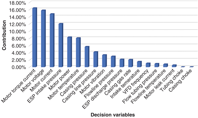
Figure 11.6 Well E52ST1’s ESP diagnostic dashboard.
Once a robust PCA model is constructed, the time at which the fracture of the pump shaft occurs could be forecasted.  and SPE equations are applied to determine the time of potential anomalies preceding the breakage of the pump shaft. Dunia and Joe Qin (1998) suggested four possible detection results under the PCA diagnostic model, those results are as follows: (1) both the
  and SPE indices exceed the control limits; (2) neither
  nor SPE indices exceed the control limits; (3) the
  index exceeds the control limit, but SPE does not; (4) the SPE index exceeds the control limit, but
  does not.
and SPE equations are applied to determine the time of potential anomalies preceding the breakage of the pump shaft. Dunia and Joe Qin (1998) suggested four possible detection results under the PCA diagnostic model, those results are as follows: (1) both the and SPE indices exceed the control limits; (2) neither nor SPE indices exceed the control limits; (3) the index exceeds the control limit, but SPE does not; (4) the SPE index exceeds the control limit, but does not.As is often the case, detection results (1) and (4) are usually regarded as potential breakage of the pump shaft. This paper contains information regarding the data of the time at which the rupture of ESP shaft occurred in each well. A detailed comparison is made between the predicted ESP’s shaft breakage time by the PCA diagnostic model and the actual ESP’s shaft breaking time.
Taking wells E52ST1, CO6ST1 and B50ST1 as examples,  and SPE indices are computed to predict the anomaly of ESP production shown in Figs. 11.7–11.9. When the ESP shaft breaks,
  and SPE are used to determine the breakage time by employing the detection results (1) and (4).
and SPE indices are computed to predict the anomaly of ESP production shown in Figs. 11.7–11.9. When the ESP shaft breaks, and SPE are used to determine the breakage time by employing the detection results (1) and (4).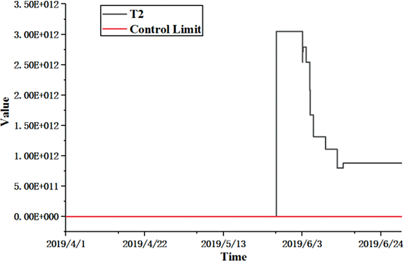
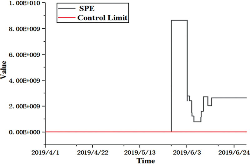
Figure 11.7 Predictions of the pump breaking time by T2 and SPE in well E52ST1.
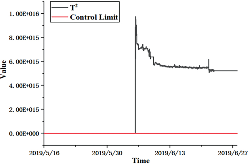
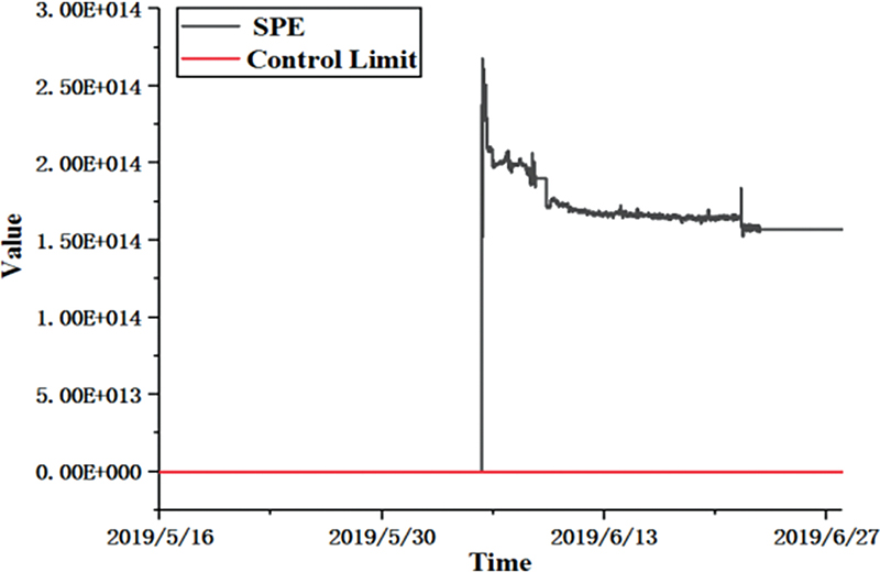
Figure 11.8 Predictions of the pump breaking time by T2 and SPE in well CO6ST1.

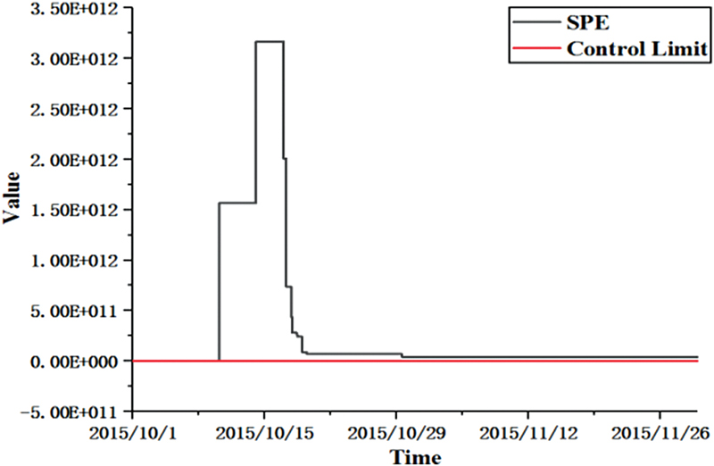
Figure 11.9 Predictions of the pump breaking time by T2 and SPE in well B48ST1.
Table 11.1 shows the comparison of the PCA diagnostic model prediction time of the pump shaft fracture and the actual ESP shaft braking time. An analysis of Table 11.1 reveals that the breakage time predicted by the PCA diagnostic model is a little earlier than the actual pump shaft breakage time. Consequently, the PCA diagnostic model has excellent accuracy in predicting the breakage time for ESP broken shaft wells and learning technique to predict the ESP broken shaft in real-time. Moreover, the PCA technique can be applied as the foundation for the development of better tools to predict ESP failure.
Table 11.1
| Wells no. | PCA model predictions | Actual breakage time |
|---|---|---|
| E52ST1 | 2019-5-26 13:40 | 2019-5-26 16:00 |
| CO6ST1 | 2019-5-27 22:20 | 2019-5-28 6:40 |
| B48ST1 | 2015-10-7 21:40 | 2015-10-8 16:20 |
| E20ST2 | 2019-9-12 10:20 | 2019-9-12 12:40 |
| B50ST2 | 2019-6-15 8:00 | 2019-6-16 15:40 |
| A11ST1 | 2015-5-10 4:40 | 2015-5-10 10:00 |
| B03ST1 | 2015-8-30 15:40 | 2015-8-31 1:00 |
| E21ST1 | 2015-8-26 10:00 | 2015-8-26 23:40 |
| E47ST1 | 2018-1-14 8:40 | 2018-1-15 9:20 |
| E42ST1 | 2018-4-24 22:40 | 2018-4-25 2:00 |
11.6. Conclusions
This paper presents a big data-driven analytical model to predict impending broken shaft in the ESP operation system. The big-data model depends on real-time data collected by ESP downhole and surface sensors. It can be concluded that PCA has the potential to be used as a recognition technique to predict dynamic changes and therefore identify the impending breakage of the ESP shaft. Key conclusions from this study can be summarized as follows:
- 1. A two-dimensional plot of scores of Principal Component 1 and Principal Component 2 can be used to identify different clusters of the stable region, unstable region, and failure region. From this two-dimensional plot, field engineers will be reminded of potential ESP shaft fracture if the cluster is far away from the stable region.
- 2. Once a robust PCA diagnostic model is built, it is of great importance that the decision variables most responsible for the breakage of the ESP shaft will be determined to explain the deviation of the cluster from the stable region.
- 3. By implementing
 and SPE equations, the PCA diagnostic model has excellent accuracy in predicting the ESP shaft breakage time.
 - 4. PCA can be used as an important pre-processing method and as an unsupervised machine learning technique to predict the developing ESP failures.
..................Content has been hidden....................
You can't read the all page of ebook, please click here login for view all page.