Search in book...
Toggle Font Controls
Create new playlist

Name your new playlist

Playlist description (optional)
Sign In

Email address

Password

Forgot Password?

or

Continue with Facebook

Continue with Google
Sign Up

Full Name

Email address

Confirm Email Address

Password

or

Continue with Facebook

Continue with Google

Chapter 12: Predictive and Diagnostic Maintenance for Rod Pumps

Patrick Bangert
Artificial Intelligence Team, Samsung SDSA, San Jose, CA, United States
algorithmica technologies GmbH, Küchlerstrasse 7, Bad Nauheim, Germany

Abstract

Approximately 20% of all oil wells in the world use a beam pump to raise crude oil to the surface. The proper maintenance of these pumps is thus an important issue in oilfield operations. We wish to know, preferably before the failure, what is wrong with the pump. Maintenance issues on the downhole part of a beam pump can be reliably diagnosed from a plot of the displacement and load on the traveling valve; a diagram known as a dynamometer card. This chapter shows that this analysis can be fully automated using machine learning techniques that teach themselves to recognize various classes of damage in advance of the failure. We use a dataset of 35292 sample cards drawn from 299 beam pumps in the Bahrain oilfield. We can detect 11 different damage classes from each other and from the normal class with an accuracy of 99.9%. This high accuracy makes it possible to automatically diagnose beam pumps in real-time and for the maintenance crew to focus on fixing pumps instead of monitoring them, which increases overall oil yield and decreases environmental impact.

Keywords

rod pumps

beam pumps

dynamometer card

oilfield operations

diagnostic maintenance

predictive maintenance

12.1. Introduction

12.1.1. Beam pumps

Of all oil wells worldwide, approximately 50% have some form of artificial lift system installed. Of those, approximately 40% make use of the beam pump, also known as the rod pump or sucker-rod pump. That accounts for approximately 500,000 beam pumps in use worldwide (Takacs, 2015). The beam pump is comprised of a standing valve at the bottom of the well, and a traveling valve attached to a rod that moves up and down the well driven by a motorized horse-head assembly on the surface, see Fig. 12.1.

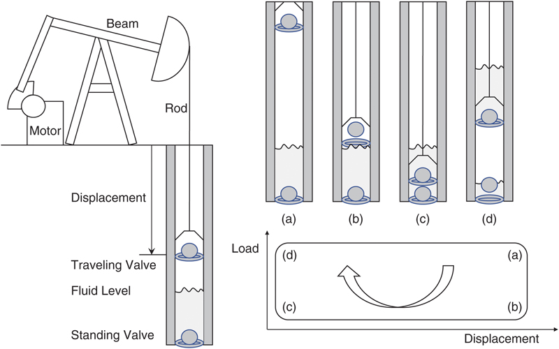
Figure 12.1 The basic schematic of a beam pump on the left with the evolution of the stroke in four stages on the right.
Plotting of displacement and load against each other over the stroke produces the dynamometer card on the bottom right.

The journey of the traveling valve from the top of the well to the bottom and back up again is called a stroke. As the pump returns to the same configuration at the start of every stroke (unless the pump breaks), the motion is inherently periodic. When the rod starts its downward journey, the standing valve closes; Fig. 12.1(a). The traveling valve opens as soon as it encounters fluid in the well and allows it to pass through; Fig. 12.1(b). At the bottom of the stroke, the traveling valve closes, and the journey is reversed at which point the standing valve opens again allowing fluid to enter the well; Fig. 12.1(c). As the closed traveling valve moves up, it transports the fluid it collected during the downstroke to the surface; Fig. 12.1(d). We can measure both the load, that is, the weight of the fluid above the traveling valve, and the displacement from the surface during one full stroke. If we graph these two variables against each other, we get a diagram known as a dynamometer card; see Fig. 12.1 bottom-right and compare with Fig. 12.2 for a real example.

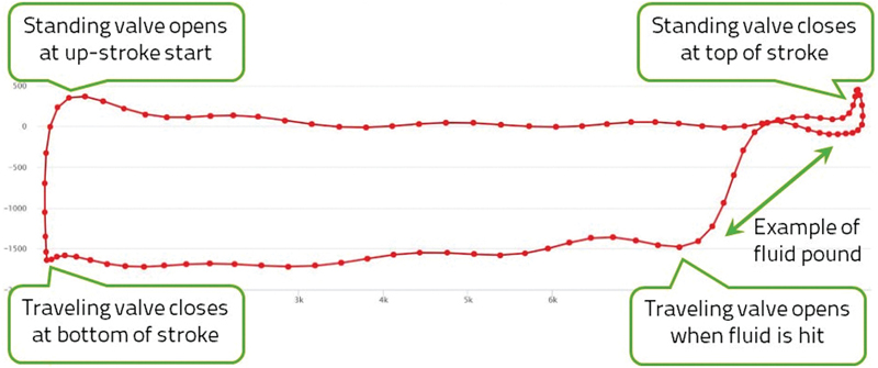
Figure 12.2 An example of a dynamometer card with the four major points labeled, see the introductory text for an explanation.

12.1.2. Beam pump problems

It was discovered by Walton Gilbert in 1936 that the shape of the dynamometer card allows an experienced person to precisely diagnose any of the typical problems that a beam pump can have downhole (Gilbert, 1936). Please see Fig. 12.3 for some examples of the various categories that are encountered. A list of typical down-hole beam pump problems follows here.

1. Normal
2. Full Pump (Fluid Friction)
3. Full Pump (Fluid Acceleration)
4. Fluid Pound (Slight)
5. Fluid Pound (Severe)
6. Pumped Off
7. Parted Tubing
8. Barrel Bent or Sticking
9. Barrel Worn or Split
10. Gas Locked
11. Gas Interference (Slight)
12. Gas Interference (Severe)
13. Traveling Valve or Plunger Leak
14. Traveling Valve Leak and Unanchored Tubing
15. Traveling and Standing Valve Balls Split in Half
16. Standing Valve Leak
17. Standing Valve Leak and Gas Interference
18. Standing Valve, Traveling Valve Leak, or Gas Interference
19. Pump Hitting Down
20. Pump Hitting Up
21. Pump Sanded Up
22. Pump Worn (Slightly)
23. Pump Worn (Severe)
24. Pump Plunger Sticking on the Upstroke
25. Pump Incomplete Fillage
26. Tubing Anchor Malfunction
27. Choked Pump
28. Hole in Barrel or Plunger Pulling out of Barrel
29. Inoperative Pump
30. Pump Hitting Up and Down
31. Inoperative Pump, Hitting Down

Figure 12.3 Some cards, obtained in the Bahrain oilfield, which illustrate that the diverse conditions of a beam pump can be visually identified.
Please see the text for a complete list of conditions. (A) Normal; (B) Fluid pound (Slight); (C) Fluid pound (Severe); (D) Pumped off; (E) Gas interference (Severe); (F) Traveling valve or plunger leak (G) Standing valve, traveling valve leak, or gas interference (H) Pump hitting down; (I) Hole in barrel or plunger pulling out of barrel (J) Inoperative pump; (K) Pump hitting up and down; (L) Inoperative pump, hitting down.

It is difficult to measure the load on the moving rod directly and so we measure it at the top of the rod and infer the downhole conditions by solving the wave equation (Bastian, 1989; Gibbs, 1963). Based on this, we can calculate several physical quantities such as a pump intake pressure without measuring them (Gibbs & Neely, 1966) and use the computed downhole card effectively to diagnose problems with the beam pump (Eickmeier, 1967). This method of determining the dynamometer card (measure at the top of the well and compute the downhole conditions) is now industry standard and relies on accurately approximating the friction laws that the moving parts experience on their journey (DaCunha and Gibbs, 2007).

12.1.3. Problem statement

The question arises: Can this diagnosis be done by a computer? If it could, then the computer would automate the diagnosis of every dynamometer card in real-time as it is measured. Depending on the stroke duration and amount of idle time, a single beam pump may produce several cards per minute. An oilfield will have hundreds or thousands of pumps. It is practically impossible for a human operator to look at them all. This automation frees up the maintenance staff to focus on fixing the pumps that need attention instead of determining which pumps need attention. It therefore decreases the environmental impact of the pump (spills, pollution, spare parts, waste, and so on) while increasing its availability and, in turn, production volume (Bangert, Tan, Zhang, & Liu, 2010).

We will demonstrate in this chapter that it is possible to reliably perform the diagnosis of a beam pump using an automatic method from machine learning that teaches itself how to distinguish the various classes of damage.

12.2. Feature engineering

Every dynamometer card in our case, has 100 load and displacement measurements over the duration of the stroke. Thus, 200 variables characterize each card and would need to be fed into whatever classification method we choose to use.

One of the first questions in every machine learning project is to determine how the available input data (in our case the 100 loads and displacements) can be transformed in order to (1) lower the number of input variables without losing any important information, and (2) bring out any quantity that we know, by expert domain knowledge, to be helpful in deciding the question at hand. This process is known as feature engineering and the resulting transformed variables are called features. Sometimes, the data obtained in the field is provided to the machine learning as it is (Sharaf, Bangert, Fardan, & Alqassab, 2019), or some of the available input variables are simply removed. This is a quite simple version of feature engineering. It is at the point of feature engineering that we have the greatest opportunity to inject domain knowledge into the machine learning task.

A model obtained by machine learning often performs significantly better on the training data for the simple reason that this data is known to it while the model is being constructed. If the model performs significantly worse on testing data, then the model cannot generalize beyond its experience to new situations and we speak of overfitting. If the model performs poorly even on training data, we speak of underfitting. Both situations are undesirable, and we look for a model that performs well on both data sets so that we may be assured that the model has learned the task that we wanted it to learn. Such a model can then be applied to new data and its conclusions become useful (Bangert, 2011).

For the problem of characterizing a dynamometer card, several papers have been published in the literature that make suggestions for suitable features. We briefly review some of these papers here and state, wherever possible, how accurately the methods performed both on the data used to construct the method (training data) and the data used to assess the method (testing data). We summarize our literature review of features in Table 12.1.

Table 12.1

A summary of the features suggested in the literature.
	Summary	Type	Cards to learn	Cards to test	Test error	References
1.	Metric is sum of differences in both dimensions	Library	—	—	—	Keating et al. (1991)
2.	Fourier series or gray level	Library	—	—	—	Dickinson and Jennings (1990)
3.	Geometric moments	Library	—	—	2.6%	Abello et al. (1993)
4.	Fourier series and geometric characteristics	Library	—	1500	13.4%	de Lima et al. (2012)
5.	Extremal points	Library	?	2166	5%	Schnitman et al. (2003)
6.	Average over segments	Model	2400	3701	2.2%	Bezerra Marco et al. (2009); Souza et al. (2009)
7.	Centroid and geometric characteristics	Model	230	100	11%	Gao et al. (2015)
8.	Fourier series	Model	102	?	5%	de Lima et al. (2009)
9.	Line angles	Segment	6132	?	24%	Reges Galdir et al. (2015)
10.	Statistical moments	Segment	88	40	2%	Li et al. (2013a)
11.	Geometric characteristics	Segment	—	—	—	Li et al. (2013a)

12.2.1. Library-based methods

A prominent idea in the older literature is that of a library. A library is a set of cards with known classification. The idea is then to compute a distance function, called a metric, between the card that we are interested in and each member of the library. The library card with the smallest distance is selected and its classification becomes the classification of the new card. This approach relies on selecting representative examples of classes for the library. It is limited by the fact that the library cannot be large if this procedure is to be carried out in real-time. The most difficult element is choosing the metric.

In one case, the library contains 37 cards and the metric is the sum of differences between the loads and displacements of the two cards being compared (Keating, Laine, & Jennings, 1991).

Another paper suggests measuring the difference between coefficients in the Fourier series representation of the card or to use a form of gray-level analysis on the image produced by a plot of the card (Dickinson and Jennings, 1990). Here the library contained 28 cards. While the authors claim that the methods performed well, we do not know the number of test cases.

Note that it makes sense to describe a dynamometer card by a Fourier series, as it is inherently periodic. If we take each measurement of displacement

x s)

and load

y s)

where

s

is a parametric variable that indexes the various measurements around one card. We can then form the complex variable

u s) = x s) + i y s)

and expand it in a Fourier series

$u s) = \sum_{n = - M}^{M} a_{n} e x p \frac{2 π i n s}{S})$

where

S

is the total card perimeter and

M

is the number of moments. The Fourier coefficients

a_{n}

are

$a_{n} = \frac{1}{S} \int_{0}^{S} u s) e x p \frac{- 2 π i n s}{S}) d s$

One may also describe the cards by geometric moments and threshold the differences to determine the most similar library member (Abello, Houang, & Russell, 1993). This approach yields a 2.6% test error on synthetically generated cards.

Geometric characteristics and Fourier series were evaluated in another study that found Fourier series to be more representative (de Lima, Guedes, Affonso, & Silva Diego, 2012). This study used 1500 cards and obtained an error of 13.4%.

An interesting approach is the attempt to extract from a card some few important points that act as local extrema and to compare them to similar points on the library cards (Schnitman, Albuquerque, Correa, Lepikson, & Bitencourt, 2003). This approach was evaluated using 2166 cards and seems to achieve an error of 5% but this is hard to quantify based on the description.

12.2.2. Model-based methods

Some features are very simplified. For instance (Bezerra Marco, Schnitman, Barreto Filho, & de Souza, 2009; Souza, Felippe, Bezerra Marco, Schnitman, & Barreto Filho, 2009) breaks the card into 32 segments and takes an average load over each segment. They had 8 different classes with 300 training examples each, 6101 manually classified cards in total and achieved a test error of 2.2%.

Another idea is to locate the centroid of the card and to compute the total area above and below the card in an extremal rectangle drawn around the card (Gao, Sun, & Liu, 2015). They then used extreme learning machines, a form of single-layer perceptron neural network, to train on 230 cards and test on 100 cards to obtain an error of 11% where we cannot be sure whether this is a total error or a test error. The centroid is

$\bar{x}, \bar{y}) = \frac{1}{N} \sum_{i = 1}^{N} x_{i}, \frac{1}{N} \sum_{i = 1}^{N} y_{i})$

Decomposing the card into a Fourier series and using the coefficients of the first moments is another idea to lower the number of dimensions. Using this, one paper reports a 5% error on 102 known cards (de Lima, Guedes, & Silva, 2009). However, it is not clear what method they used to classify the cards and how many of the cards were used for training and testing.

12.2.3. Segment-based methods

Some proposals depend upon the ability to detect the four points on a card at which the standing and traveling valves open and close, see Fig. 12.2. There are two methods to determine those points. One relies on a pure geometric interpretation called the chain code (Reges Galdir, Schnitman, & Reis, 2014) and another on a physically motivated heuristic (Hua and Xunming, 2011). Supposing that we can determine these opening and closing points, we may then proceed to compute some quantities for each of the four segments of the card.

One paper suggests three geometric quantities based on the angle between the straight lines between any two neighboring pairs of observations (Reges Galdir, Schnitman, Reis, & Mota, 2015). They then build a fuzzy logic classifier for each one of 11 classes. Having 6132 manually classified cards in total, it appears from the unclear description that the error was approximately 24%. As the paper does not break its data into training and test, the test error would be higher than that.

Another approach requiring the opening and closing points is to compute the first seven statistical moments of the data in each segment (Li, Gao Xian, Yang Wei, Dai Ying, & Tian, 2013a). They use support vector machines to learn from 88 training cards and 40 test cards to obtain a test error of 2%. Another paper uses geometric characteristics of the four segments and claims effective performance using a simple look-up table of which class has or does not have which characteristic, but the authors provide no numerical results (Li, Gao Xian, Tian & Qiu, 2013b).

12.2.4. Other methods

A completely different approach is to try to extract knowledge and experience of human experts into the form of rules, usually known as an expert system. These rules would have to be formulated in precise numerical terms, so they can be evaluated on a card in an automated computer system. This has been done for this task and the management process is discussed of how one obtains these rules (Alegre, de Rocha, & Morooka, 1993). The authors do not report on the accuracy of the system.

Notably, one paper claims to have achieved perfect classification results on 6113 manually classified cards (Reges, Schnitman, & Reis, 2013). As they do not describe their features, their classification method, or in what manner, if any, they divided the data set into a training and testing data set, it is difficult to evaluate this result.

12.2.5. Selection of features

We have attempted each of the above referenced feature methodologies. Our conclusion is that the automatic detection of the four-valve opening and closing points is numerically unstable in general and particularly for non-normal dynamometer cards that are, of course, of particular interest to this application. Thus, we have decided to exclude all the features that require this basis.

In selecting features, we must make a trade-off between bias and variance (Dong and Liu, 2018; Zheng and Casari, 2018). A high bias means that the test error is high, and a high variance means that the variance of the test error is high across several runs of the algorithm with different training and testing data sets. A smaller number of features will generally lower the test error but increase the variance while a small number of features will remove essential information from the problem and thus increase the test error. We must therefore select the right number of features to characterize the situation with enough (bias) but not too much (variance) detail.

Having several candidate features available for selection, we would hope to rank them and take the first few features that contribute most to the task at hand. Unfortunately, this simple approach is generally doomed to failure. A central result in the field of feature engineering is that a feature that is insignificant on its own can provide significant performance increases together with other features, and two features that are both insignificant individually may be significant together. Therefore, we must not select features individually but rather in groups. This is problematic in the case, as it is here, that we have many features to choose from and the number of combinations of features is too large to try in a realistic amount of computation time. For each combination, we must train the model several times as we need to know not only the performance but the variance of any selected set of features. The normal way to solve this problem is with so-called wrapper methods that train a simple model for each combination to save overall computation time. The selected feature set is then used to train the complex model (Guyon and Elisseeff, 2003).

For example, the method of representing the dynamometer card by its Fourier series leads to many numerical experiments as the number of moments in the series must be chosen. To illustrate the trade-off, we plot the bias and variance in Fig. 12.4. The plot is a standard box-and-whisker-plot for various scenarios. The vertical axis represents the number of test errors obtained with a model trained on 30000 cards and tested on 5292 cards. Each time a model is trained, the training and test examples are chosen at random. All models that went into the figure exhibited zero training errors. The vertical position of the box on the plot, the average number of test errors over 5 models, is the bias. The vertical size of the box is a representation of the variance. The first 13 boxes correspond to representing the card by the Fourier series of that many moments, starting with zero moments. The seven boxes after that, labeled S1 through S7, correspond to various other combinations,

• S1: Fourier series with 1 moment and all 5 geometrical features of (Gao et al., 2015).
• S2: The 5 geometrical features of (Gao et al., 2015).
• S3: The centroid coordinates of the card.
• S4: The centroid coordinates and the average line length.
• S5: Fourier series with 1 moment, the centroid coordinates, and the average line length.
• S6: Fourier series with 1 moment and the centroid coordinates.
• S7: Fourier series with 1 moment, the centroid coordinates, and the two area integrals.

Figure 12.4 An illustration of the bias-variance trade-off in choosing the number of moments in a Fourier series representation of a dynamometer card.
See text for an explanation.

From these experiments, we can conclude that a Fourier series of 4 moments has the least variance but this is achieved at a significant cost in bias. The Fourier series of 1 moment has the least bias but this is achieved at a cost in variance. The Fourier series of 1 moment in combination with the centroid coordinates (option S6) offers the best compromise with 12 test errors on average with a standard deviation of 4. This implies a test error rate of 0.0023 ± 0.0008 or an accuracy rate of 99.8 ± 0.1%. The best single model encountered, overall and with the S6 feature combination, only exhibited 7 test errors (accuracy of (5292 – 7)/5292 x 100% = 99.9%). It is this model that we have chosen to put into production.

In conclusion, our investigation of feature engineering yields that the best features are the Fourier series coefficients to the first moment and the coordinates of the centroid of the card. We therefore have five features. While this may be surprising due to its simplicity, it does lead to very good classification results. In comparison to the papers cited above, this study uses a far larger dataset both to train the model as well as to test its performance.

12.3. Project method to validate our model

12.3.1. Data collection

We must measure some cards in the field. This was done on 299 of the approximately 750 different beam pumps distributed in the Bahrain oilfield all of which are instrumented, and the data is relayed by a digital canopy to a central data facility where the cards can be obtained in real-time and saved to a database. In total 5,380,163 cards were collected for a first study during the fall of 2018.

12.3.2. Generation of training data

Some training data must be generated. The operating company of the Bahrain oilfield, Tatweer Petroleum, has four experts on its staff who are responsible for determining maintenance activities based on dynamometer cards. These experts were asked to look at the cards measured and to classify them into the classes mentioned above. Over a few weeks, they classified 35,292 dynamometer cards. These cards make up the dataset that can be used to both train the machine learning model and to determine its effectiveness.

12.3.3. Feature engineering

We computed the features for each dynamometer card; see the discussion of feature engineering earlier. We also divided the 35,292 known cards into two groups. 85% of the cards were used to train the model and 15% were used to assess the model after training. These two data sets are usually called the training data and the testing data.

12.3.4. Machine learning

We presented the training data set to several machine learning algorithms. Each algorithm has parameters that a human expert must tune experimentally to the task. We performed parameter tuning in each case to get the best performance out of each algorithm type. We attempted a single-layer perceptron neural network (Goodfellow, Bengio, & Courville, 2016), multiple-layer perceptron neural network (Goodfellow et al., 2016), extreme learning (Gao et al., 2015), and decision trees (Breiman, Friedman, Stone Charles, & Olshen, 1984).

The stochastic gradient-boosted decision tree is the most effective method for this task. It shows perfect performance on the training data set and 99.9% accuracy on the testing data set. The errors that it makes on the testing data set are roughly evenly distributed among the various classes, which is another desirable fact, see Table 12.2. Some other algorithms were competitive on the error rate but clustered its errors in one or other of the classes, which showed a systematic problem with detecting that class accurately.

Table 12.2

Classification performance of the best model on the test data set.
Category	Training samples	Testing samples	Incorrect
Normal	8557	1529	0
Fluid pound (Slight)	5347	955	0
Fluid pound (Severe)	93	15	0
Inoperative pump	1981	379	0
Pump hitting down	1740	303	2
Pump hitting up and down	2258	407	2
Inoperative pump, hitting down	9045	1626	1
Traveling valve or plunger leak	98	15	1
Standing valve, traveling valve leak, or gas interference	345	62	0
Pumped off	234	39	1
Hole in barrel or plunger pulling out of barrel	132	20	0
Gas interference (Severe)	101	11	0
Total	29931	5361	7

For each class, we specify how many training and testing samples were used. The model performed perfectly on all training samples but made a few errors on testing samples, as specified.

12.3.5. Summary of methodology

The entire procedure of generating and using the classification model is summarized in Fig. 12.5. The workflow on the bottom of the figure describes the production situation in which a dynamometer card is measured, its features extracted, and its classification computed by the existing classification model. The model itself is a formula that takes a card’s features as input and produces a class number as output using several parameters that have been learned. The workflow at the top of the figure produces the model, which is nothing more than computing the parameters of the formula that will be the model in the end. This learning procedure uses card features and the known classification, produced by human experts, of those cards. This schematic workflow is always the same for the general problem of classification, no matter what type of raw data, feature engineering, or model type we choose to use.

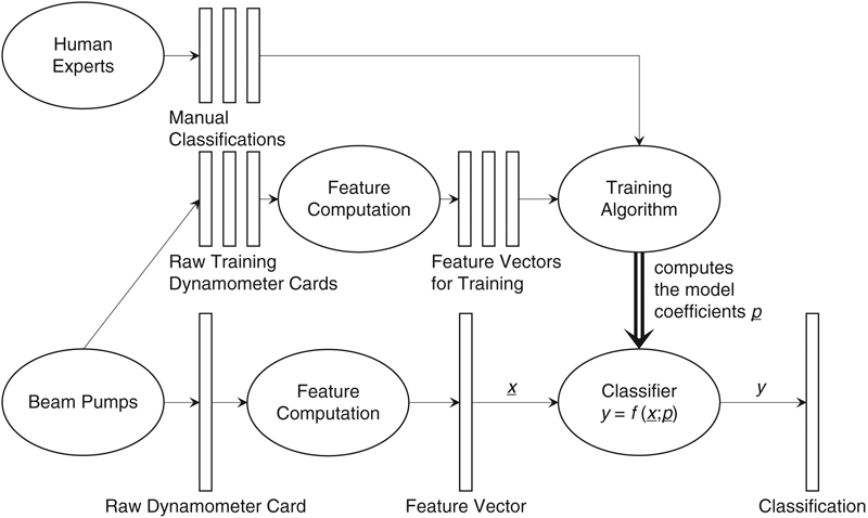
Figure 12.5 Elements of the diagnosis procedure.

12.4. Results

12.4.1. Summary and review

Based on 35292 manually classified cards, we performed feature engineering to determine that the best set of features to balance between bias and variance of the model is to take the Fourier series representation of the card to the first moment and to take the centroid coordinates of the card. We found that computationally detecting the four-valve opening and closing points of the traveling and standing valves as proposed in the literature is numerically unstable and so the features depending on this basis were not investigated. Using 85% of the data for training and 15% for testing, we obtained a model that makes no training errors and 7 test errors. This performance can be reproduced over multiple training runs, where each training run chooses the training and testing samples randomly, with a variance of 4 test errors. The distribution of test errors across the different classes is relatively even, so that we seem not to be making a systematic error, see Table 12.2.

12.4.2. Conclusion

We conclude that the classification accuracy is high enough for the model to be used practically to identify the various beam pump problems in a real oilfield. It can do this in real-time for many beam pumps simultaneously and thus offer a high degree of automation in the detection of problems. If a card is identified as non-normal, the method will release an automated alert with its diagnosis and thus generate a maintenance measure. This procedure frees up human experts from the job of monitoring and diagnosing beam pumps to the more important task of fixing them. It also alerts the experts sooner than they would have discovered the problems by themselves as the algorithm can diagnose every dynamometer card as it is measured; a volume of analysis that would be impossible for a human team of realistic size.

We note that this work can classify cards into one of 12 classes. We have identified 31 classes in principle. The existing model will not work for the remaining 19 classes, as we did not have any training samples for them. When these problems occur on real beam pumps in the field, the relevant cards should be manually classified and then the training process can be repeated to expand the model’s classification ability beyond its current domain. We estimate that about 100 samples per class are necessary to achieve reasonable results for that class. It is however clear that more data will always lead to either a more accurate or a more robust model. No matter how mature the model, feedback by manual classification is always of value.

..................Content has been hidden....................

You can't read the all page of ebook, please click here login for view all page.

Table of Contents for Chapter 12: Predictive and Diagnostic Maintenance for Rod Pumps

Create new playlist

Sign In

Sign Up