Chapter 8 Multiple Reactions

Search in book...
Toggle Font Controls
Create new playlist

Name your new playlist

Playlist description (optional)
Sign In

Email address

Password

Forgot Password?

or

Continue with Facebook

Continue with Google
Sign Up

Full Name

Email address

Confirm Email Address

Password

or

Continue with Facebook

Continue with Google

Multiple Reactions 8

Sometimes you just have to jump and build your wings on the way down.

—Carol Craig, entrepreneur

Overview. Seldom is the reaction of interest the only one that occurs in a chemical reactor. Typically multiple reactions will occur, some desired and some undesired. One of the key factors in the economic success of a chemical plant is the minimization of undesired side reactions that occur along with the desired reaction.

In this chapter, we discuss reactor selection and general mole balances, net rates, and relative rates for multiple reactions.

First, we describe the four basic types of multiple reactions:

• Series

• Parallel

• Independent

• Complex

Next, we define the selectivity parameter and discuss how it can be used to minimize unwanted side reactions by proper choice of operating conditions and reactor selection.

We then show how to modify our CRE algorithm to solve reaction engineering problems when multiple reactions are involved. The modification builds on the algorithm presented in Chapter 6 by numbering all reactions and expanding the Rates Building Block into three parts:

• Rate laws

• Relative rates

• Net rates

Finally, a number of examples are given that show how the algorithm is applied to real reactions.

8.1 Definitions

8.1.1 Types of Reactions

There are four basic types of multiple reactions: parallel, series, independent, and complex. These types of multiple reactions can occur by themselves, in pairs, or all together. When there is a combination of parallel and series reactions, they are often referred to as complex reactions.

Parallel reactions (also called competing reactions) are reactions where the reactant is consumed by two different reaction pathways to form different products:

Parallel reactions

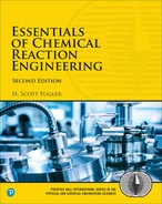
An example of an industrially significant parallel reaction is the oxidation of ethylene to ethylene oxide while avoiding complete combustion to carbon dioxide and water:

Serious chemistry

Series reactions (also called consecutive reactions) are reactions where the reactant forms an intermediate product, which reacts further to form another product:

Series reactions

A \overset{k_{1}}{\to} B \overset{k_{2}}{\to} C

$A \overset{k_{1}}{\to} B \overset{k_{2}}{\to} C$

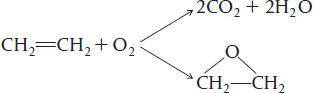
An example of a series reaction is the reaction of ethylene oxide (EO) with ammonia to form mono-, di-, and triethanolamine:

In recent years, the shift has been toward the production of diethanolamine as the desired product rather than triethanolamine.

Independent reactions are reactions that occur at the same time but neither the products nor the reactants react with themselves or one another.

Independent reactions

\begin{matrix} A \to B + C \\ D \to E + F \end{matrix}

$\begin{matrix} A \to B + C \\ D \to E + F \end{matrix}$

An example is the cracking of crude oil to form gasoline, where two of the many reactions occurring are

C₁₅H₃₂ → C₁₂C₂₆ + C₃H₆

C₈H₁₈ → C₆H₁₄ + C₂H₄

Complex reactions are multiple reactions that involve combinations of series and independent parallel reactions, such as

A + B → C + D

A + C → E

E → G

An example of a combination of parallel and series reactions is the formation of butadiene from ethanol:

C₂H₅OH → C₂ H₄ + H₂O

C₂H₅OH → CH₃CHO+H₂

C₂H₄ + CH₃CHO → C₄H₆+H₂O

8.1.2 Selectivity

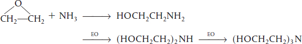
Desired and Undesired Reactions. Of particular interest are reactants that are consumed in the formation of a desired product, D, and the formation of an undesired product, U, in a competing or side reaction. In the parallel reaction sequence

\begin{matrix} A \overset{k_{D}}{\to} D \\ A \overset{k_{U}}{\to} U \end{matrix}

$\begin{matrix} A \overset{k_{D}}{\to} D \\ A \overset{k_{U}}{\to} U \end{matrix}$

or in the series reaction sequence

A \overset{k_{D}}{\to} D \overset{k_{U}}{\to} U

$A \overset{k_{D}}{\to} D \overset{k_{U}}{\to} U$

The economic incentive

we want to minimize the formation of U and maximize the formation of D because the greater the amount of undesired product formed, U, the greater the cost of separating the undesired product U from the desired product D (see Figure 8-1).

Figure shows a rightward arrow from A pointing to a reactor system that further leads to a test tube labeled "Separator." An upward arrow labeled "D" and a downward arrow labeled "U" from the separator point to the right.

Figure 8-1 Reaction-separation system producing both desired and undesired products.

Selectivity tells us how one product is favored over another when we have multiple reactions. We can quantify the formation of D with respect to U by defining the selectivity and the yield of the system. The instantaneous selectivity of D with respect to U is the ratio of the rate of formation of D to the rate of formation of U.

Instantaneous selectivity

$\begin{matrix} S_{D/U} = \frac{r_{D}}{r_{U}} = \frac{rate of formation of D}{rate of formation of U} & \begin{matrix} (8 - 1) \end{matrix} \end{matrix}$ $\begin{matrix} S_{D/U} = \frac{r_{D}}{r_{U}} = \frac{rate of formation of D}{rate of formation of U} & \begin{matrix} (8 - 1) \end{matrix} \end{matrix}$

In Section 8.3, we will see how evaluating S_D/u will guide us in the design and selection of our reaction system to maximize the selectivity.

Another definition of selectivity used in the current literature, ${\tilde{S}}_{D/U}$ ${\tilde{S}}_{D/U}$ , is given in terms of the flow rates leaving the reactor. ${\tilde{S}}_{D/U}$ ${\tilde{S}}_{D/U}$ is the overall selectivity.

Overall selectivity

$\begin{matrix} {\tilde{S}}_{D/U} = \frac{F_{D}}{F_{U}} = \frac{Exit molar flow rate of desired product}{Exit molar flow rate of undesired product} & \begin{matrix} (8 - 2 a) \end{matrix} \end{matrix}$ $\begin{matrix} {\tilde{S}}_{D/U} = \frac{F_{D}}{F_{U}} = \frac{Exit molar flow rate of desired product}{Exit molar flow rate of undesired product} & \begin{matrix} (8 - 2 a) \end{matrix} \end{matrix}$

Using a CSTR mole balance on species D and on species U, it is easily shown that for a CSTR the instantaneous and overall selectivities are identical, i.e., SD/U ⁼ ${\tilde{S}}_{D/U}$ ${\tilde{S}}_{D/U}$ See the Chapter 8 Expanded Material on the CRE Web site http://www.umich.edu/~elements/5e/08chap/expanded.html.

For a batch reactor, the overall selectivity is given in terms of the number of moles of D and U at the end of the reaction time.

$\begin{matrix} {\tilde{S}}_{D/U} = \frac{N_{D}}{N_{U}} & \begin{matrix} (8 - 2 b) \end{matrix} \end{matrix}$ $\begin{matrix} {\tilde{S}}_{D/U} = \frac{N_{D}}{N_{U}} & \begin{matrix} (8 - 2 b) \end{matrix} \end{matrix}$

Two definitions for selectivity and yield are found in the literature.

8.1.3 Yield

Reaction yield, like selectivity, has two definitions: one based on the ratio of reaction rates and one based on the ratio of molar flow rates. In the first case, the yield at a point can be defined as the ratio of the reaction rate of a given product to the reaction rate of the key reactant A, usually the basis of calculation. This yield is referred to as the instantaneous yield Y_D.

$\begin{matrix} Y_{D} = \frac{r_{D}}{- r_{A}} & \begin{matrix} (8 - 3) \end{matrix} \end{matrix}$ $\begin{matrix} Y_{D} = \frac{r_{D}}{- r_{A}} & \begin{matrix} (8 - 3) \end{matrix} \end{matrix}$

Instantaneous yield based on reaction rates

The overall yield, ${\tilde{Y}}_{D}$ ${\tilde{Y}}_{D}$ , is based on molar flow rates and defined as the ratio of moles of product formed at the end of the reaction to the number of moles of the key reactant, A, that have been consumed.

For a batch system

$\begin{matrix} {\tilde{Y}}_{_{D}} = \frac{N_{D}}{N_{A 0} - N_{A}} & (8 - 4 a) \end{matrix}$ $\begin{matrix} {\tilde{Y}}_{_{D}} = \frac{N_{D}}{N_{A 0} - N_{A}} & (8 - 4 a) \end{matrix}$

Overall yield based on moles

For a flow system

$\begin{matrix} {\tilde{Y}}_{_{D}} = \frac{F_{D}}{F_{A 0} - F_{A}} & (8 - 4 b) \end{matrix}$ $\begin{matrix} {\tilde{Y}}_{_{D}} = \frac{F_{D}}{F_{A 0} - F_{A}} & (8 - 4 b) \end{matrix}$

Overall yield based on molar flow rates

As with selectivity, the instantaneous yield and the overall yield are identical for a CSTR (i.e., ${\tilde{Y}}_{D}$ ${\tilde{Y}}_{D}$ = Y_D). From an economic standpoint, the overall selectivities, $\tilde{S}$ $\tilde{S}$ , and yields, $\tilde{Y}$ $\tilde{Y}$ , are important in determining profits, while the instantaneous selectivities give insights in choosing reactors, operating conditions, and reaction schemes that will help maximize the profit. There often is a conflict between selectivity and conversion because you want to make as much as possible of your desired product (D) and at the same time minimize the undesired product (U). However, in many instances, the greater the conversion you achieve, not only do you make more D, but you also form more U.

8.1.4 Conversion

While we will not code or solve multiple reaction problems using conversion, it sometimes gives insight to calculate it from the molar flow rates or the number of moles. However, to do this we need to give conversion X a subscript to refer to one of the reactants fed.

For Species A

$\begin{matrix} \overset{Flow}{X_{A} = \frac{F_{A0} - F_{A}}{F_{A0}}} & or & \overset{Batch}{X_{A} = \frac{N_{A0} - N_{A}}{N_{A0}}} & (8 - 5 a) \end{matrix}$ $\begin{matrix} \overset{Flow}{X_{A} = \frac{F_{A0} - F_{A}}{F_{A0}}} & or & \overset{Batch}{X_{A} = \frac{N_{A0} - N_{A}}{N_{A0}}} & (8 - 5 a) \end{matrix}$

and for Species B

$\begin{matrix} \overset{Flow}{X_{B} = \frac{F_{B0} - F_{B}}{F_{B0}}} & or & \overset{Batch}{X_{B} = \frac{N_{B0} - N_{B}}{N_{B0}}} \end{matrix}$ $\begin{matrix} \overset{Flow}{X_{B} = \frac{F_{B0} - F_{B}}{F_{B0}}} & or & \overset{Batch}{X_{B} = \frac{N_{B0} - N_{B}}{N_{B0}}} \end{matrix}$

For a semibatch reactor where B is fed to A

$\begin{matrix} X_{A} = \frac{C_{A0} V_{0} - C_{A} V}{C_{A0} V_{0}} & (8 - 5 b) \\ X_{B} = \frac{F_{B0} t - C_{B} V}{F_{B0} t}, for e .g .,t > 0 .001 s & (8 - 5 c) \end{matrix}$ $\begin{matrix} X_{A} = \frac{C_{A0} V_{0} - C_{A} V}{C_{A0} V_{0}} & (8 - 5 b) \\ X_{B} = \frac{F_{B0} t - C_{B} V}{F_{B0} t}, for e .g .,t > 0 .001 s & (8 - 5 c) \end{matrix}$

The conversion for the different species fed is easily included in the numerical software solutions.

8.2 Algorithm for Multiple Reactions

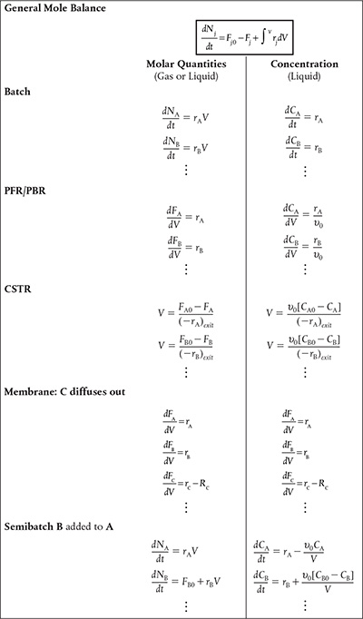
The multiple-reaction algorithm can be applied to parallel reactions, series reactions, independent reactions, and complex reactions. The availability of software packages (ODE solvers) makes it much easier to solve problems using moles Nj or molar flow rates F_;· rather than conversion. For liquid systems, concentration is usually the preferred variable used in the mole balance equations.

After numbering each and every reaction involved we carry out a mole balance on each and every species. The mole balances for the various types of reactors we have been studying are shown in Table 8-1. The rates shown Table 8-1, e.g., r_A, are the net rates of formation and are discussed in detail in Table 8-2. The resulting coupled differential mole balance equations can be easily solved using an ODE solver. In fact, this section has been developed to take advantage of the vast number of computational techniques now available on laptop computers (e.g., Polymath).

TABLE 8-1 MOLE BALANCES FOR MULTIPLE REACTIONS

Mole balances on every species

Just a very few changes to our CRE algorithm for multiple reactions

8.2.1 Modifications to the Chapter 6 CRE Algorithm for Multiple Reactions

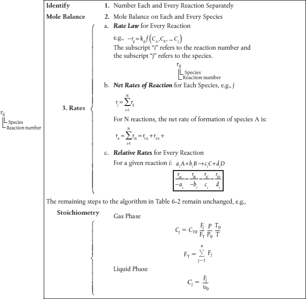
There are a few small changes to the CRE algorithm presented in Table 6-2, and changes to our CRE _we _wj|| describe these changes in detail when we discuss complex reactions in pie reactions Section 8.5. However, before discussing parallel and series reactions, it is necessary to point out some of the modifications to our algorithm. These changes are highlighted by brackets in Table 8-2. When analyzing multiple reactions, we first number every reaction. Next, we must perform a mole balance on each and every species, just as we did in Chapter 6 to analyze reactions in terms of the mole balances for different reactor types. The rates of formation shown in the mole balances in Table 6-2 (e.g., r_A, r_B, rj) are the net rates of formation. The main change in the CRE algorithm in Table 6-2 is that the Rate Law step in our algorithm has now been replaced by the step Rates, which includes three substeps:

• Rate Laws

• Net Rates

• Relative Rates

The concentrations identified in the lower bracket in Table 8-2 are the same concentrations that were discussed in Chapter 6.

TABLE 8-2 MODIFICATION TO THE CRE ALGORITHM

8.3 Parallel Reactions

8.3.1 Selectivity

In this section, we discuss various means of minimizing the undesired product, U, through the selection of reactor type and operating conditions. We also discuss the development of efficient reactor schemes.

For the competing reactions such as

\begin{matrix} (1) & A \overset{k_{D}}{\to} D & (Desired) \\ (2) & A \overset{k_{U}}{\to} U & (Undesired) \end{matrix}

$\begin{matrix} (1) & A \overset{k_{D}}{\to} D & (Desired) \\ (2) & A \overset{k_{U}}{\to} U & (Undesired) \end{matrix}$

the rate laws are

Rate laws for formation of desired and undesired products

\begin{matrix} r_{D} = k_{D} C_{A}^{α_{1}} & (8-6) \end{matrix}

$\begin{matrix} r_{D} = k_{D} C_{A}^{α_{1}} & (8-6) \end{matrix}$

\begin{matrix} r_{U} = k_{U} C_{A}^{α_{2}} & (8-7) \end{matrix}

$\begin{matrix} r_{U} = k_{U} C_{A}^{α_{2}} & (8-7) \end{matrix}$

The net rate of disappearance of A for this reaction sequence is the sum of the rates of formation of U and D:

- \begin{matrix} r_{A} = r_{D} + r_{U} & (8-8) \end{matrix}

$- \begin{matrix} r_{A} = r_{D} + r_{U} & (8-8) \end{matrix}$

- \begin{matrix} r_{A} = k_{D} C_{A}^{α_{1}} + k_{U} C_{A}^{α_{2}} & (8-9) \end{matrix}

$- \begin{matrix} r_{A} = k_{D} C_{A}^{α_{1}} + k_{U} C_{A}^{α_{2}} & (8-9) \end{matrix}$

where α₁ and α₂ are positive reaction orders. We want the rate of formation of D, r_D, to be high with respect to the rate of formation of U, r_O. Taking the ratio of these rates [i.e., Equation (8-6) to Equation (8-7)], we obtain the instantaneous selectivity, S_D/_U, which is to be maximized:

Instantaneous selectivity

\begin{matrix} S_{D/U} = \frac{r_{D}}{r_{U}} = \frac{k_{D}}{k_{U}} C_{A}^{α_{1} - α_{2}} & (8-10) \end{matrix}

$\begin{matrix} S_{D/U} = \frac{r_{D}}{r_{U}} = \frac{k_{D}}{k_{U}} C_{A}^{α_{1} - α_{2}} & (8-10) \end{matrix}$

8.3.2 Maximizing the Desired Product for One Reactant

In this section, we examine ways to maximize the instantaneous selectivity, ${\overset{}{S}}_{D/U}$ ${\overset{}{S}}_{D/U}$ , for different reaction orders of the desired and undesired products.

Case 1: α_λ > α₂. The reaction order of the desired product, α_1; is greater than the reaction order of the undesired product, α₂. Let a be a positive number that is the difference between these reaction orders (a > 0):

α₁ – α₂ = a

For α₁ > α₂ , make C_A as large as possible by using a PFR or batch reactor.

Then, upon substitution into Equation (8-10), we obtain

\begin{matrix} S_{D/U} = \frac{r_{D}}{r_{U}} = \frac{k_{D}}{k_{U}} C_{A}^{a} & (8-11) \end{matrix}

$\begin{matrix} S_{D/U} = \frac{r_{D}}{r_{U}} = \frac{k_{D}}{k_{U}} C_{A}^{a} & (8-11) \end{matrix}$

To make this ratio as large as possible, we want to carry out the reaction in a manner that will keep the concentration of reactant A as high as possible during the reaction. If the reaction is carried out in the gas phase, we should run it without inerts and at high pressures to keep C_A high. If the reaction is in the liquid phase, the use of diluents should be kept to a minimum.¹

¹ For a number of liquid-phase reactions, the proper choice of a solvent can enhance selectivity. See, for example, Ind. Eng. Chem., 62(9), 16. In gas-phase heterogeneous catalytic reactions, selectivity is an important parameter of any particular catalyst.

A batch or plug-flow reactor should be used in this case because, in these two reactors, the concentration of A starts at a high value and drops progressively during the course of the reaction. In a perfectly mixed CSTR, the concentration of reactant within the reactor is always at its lowest value (i.e., that of the outlet concentration) and therefore the CSTR should not be chosen under these circumstances.

Case 2: α₂ > α₁. The reaction order of the undesired product is greater than that of the desired product. Let b = α₂ – α₁, where b is a positive number; then

\begin{matrix} S_{D/U} = \frac{r_{D}}{r_{U}} = \frac{k_{D} C_{A}^{α 1}}{k_{U} C_{A}^{α_{2}}} = \frac{k_{D}}{k_{U} C_{A}^{α_{2} - α_{1}}} = \frac{k_{D_{}}}{k_{U} C_{A}^{b}} & (8-12) \end{matrix}

$\begin{matrix} S_{D/U} = \frac{r_{D}}{r_{U}} = \frac{k_{D} C_{A}^{α 1}}{k_{U} C_{A}^{α_{2}}} = \frac{k_{D}}{k_{U} C_{A}^{α_{2} - α_{1}}} = \frac{k_{D_{}}}{k_{U} C_{A}^{b}} & (8-12) \end{matrix}$

For the ratio r_D/r_U to be high, the concentration of A should be as low as possible.

For α₂ > α₁ use a CSTR and dilute the feed stream.

This low concentration may be accomplished by diluting the feed with inerts and running the reactor at low concentrations of species A. A CSTR should be used because the concentrations of reactants are maintained at a low level. A recycle reactor in which the product stream acts as a diluent could be used to maintain the entering concentrations of A at a low value.

Because the activation energies of the two reactions in cases 1 and 2 are not given, it cannot be determined whether the reaction should be run at high or low temperatures. The sensitivity of the rate selectivity parameter to temperature can be determined from the ratio of the specific reaction rates

\begin{matrix} S_{D/U} \sim \frac{k_{D}}{k_{U}} = \frac{A_{D}}{A_{U}} e^{- [(E_{D} - E_{U}) / RT]} & (8-13) \end{matrix}

$\begin{matrix} S_{D/U} \sim \frac{k_{D}}{k_{U}} = \frac{A_{D}}{A_{U}} e^{- [(E_{D} - E_{U}) / RT]} & (8-13) \end{matrix}$

Effect of temperature on selectivity

where A is the frequency factor and E the activation energy, and the subscripts D and U refer to desired and undesired product, respectively.

Case 3: E_D > Ε_υ. In this case, the specific reaction rate of the desired reaction fe_D (and therefore the overall rate r_D ) increases more rapidly with increasing temperature, T, than does the specific rate of the undesired reaction k_v. Consequently, the reaction system should be operated at the highest possible temperature to maximize S_D/U.

Graph shows the horizontal axis represents "T (in Kelvin), the vertical axis represents "S subscript (D over U)." An increasing concave upward curve is shown and labeled "E subscript D greater than E subscript U."

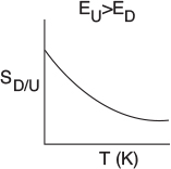
Case 4: Ε_υ > E_D. In this case, the reaction should be carried out at a low temperature to maximize S^, but not so low that the desired reaction does not proceed to any significant extent.

Graph shows the horizontal axis represents "T (in Kelvin), the vertical axis represents "S subscript (D over U)." A decreasing concave upward curve is shown and labeled "E subscript U greater than E subscript D."

Example 8-1 Maximizing the Selectivity for the Famous Trambouze Reactions

Reactant A decomposes by three simultaneous reactions to form three products, one that is desired, B, and two that are undesired, X and Y. These liquid-phase reactions, along with the appropriate rate laws, are called the Trambouze reactions (AIChE J., 5, 384).

1) $\begin{matrix} A \overset{k_{1}}{\to} X & - r_{1 A} = r_{X} = k_{1} = 0.0001 \frac{mol}{{dm}^{3} \cdot s} & (\begin{matrix} zero order \end{matrix}) \end{matrix}$ $\begin{matrix} A \overset{k_{1}}{\to} X & - r_{1 A} = r_{X} = k_{1} = 0.0001 \frac{mol}{{dm}^{3} \cdot s} & (\begin{matrix} zero order \end{matrix}) \end{matrix}$

2) $\begin{matrix} A \overset{k_{2}}{\to} B & - r_{2A} = r_{B} = k_{2} C_{A} = (0.0015 s^{- 1}) C_{A} & (\begin{matrix} first order \end{matrix}) \end{matrix}$ $\begin{matrix} A \overset{k_{2}}{\to} B & - r_{2A} = r_{B} = k_{2} C_{A} = (0.0015 s^{- 1}) C_{A} & (\begin{matrix} first order \end{matrix}) \end{matrix}$

3) $\begin{matrix} A \overset{k_{3}}{\to} Y & - r_{3A} = r_{Y} = k_{3} C_{A}^{2} = (0.008 \frac{{dm}^{3}}{mol \cdot s}) {C^{2}}_{A} & (\begin{matrix} second order \end{matrix}) \end{matrix}$ $\begin{matrix} A \overset{k_{3}}{\to} Y & - r_{3A} = r_{Y} = k_{3} C_{A}^{2} = (0.008 \frac{{dm}^{3}}{mol \cdot s}) {C^{2}}_{A} & (\begin{matrix} second order \end{matrix}) \end{matrix}$

The specific reaction rates are given at 300 K and the activation energies for reactions (1), (2), and (3) are E_l = 10,000 cal/mole, E₂ = 15,000 cal/mole, and E₃ = 20,000 cal/mole.

(a) How, and under what conditions (e.g., reactor type(s), temperature, concentrations), should the reaction be carried out to maximize the selectivity of species B for an entering concentration of species A of 0.4 M and a volumetric flow rate of 2.0 dm³/s?

(b) How could the conversion of B be increased and still keep selectivity relatively high?

Solution

Part (a)

The instantaneous selectivity of species B with respect to species X and Y is

$\begin{matrix} S_{B/XY} = \frac{r_{B}}{r_{X} + r_{Y}} = \frac{k_{2} C_{A}}{k_{1} + k_{3} C_{A}^{2}} & (E8-1 .1) \end{matrix}$ $\begin{matrix} S_{B/XY} = \frac{r_{B}}{r_{X} + r_{Y}} = \frac{k_{2} C_{A}}{k_{1} + k_{3} C_{A}^{2}} & (E8-1 .1) \end{matrix}$

When we plot S_B/XY vs. C_A, we see that there is a maximum, as shown in Figure E8-1.1.

$S_{B/XY} = \frac{r_{B}}{r_{X} + r_{Y}} = \frac{k_{2} C_{A}}{k_{1} + k_{3} C_{A}^{2}}$ $S_{B/XY} = \frac{r_{B}}{r_{X} + r_{Y}} = \frac{k_{2} C_{A}}{k_{1} + k_{3} C_{A}^{2}}$

Graph shows a curve representing selectivity as a function of the concentration of A.

Figure E8-1.1 Selectivity as a function of the concentration of A.

As we can see, the selectivity S_B/XY reaches a maximum at a concentration $C_{A}^{*}$ $C_{A}^{*}$ . Because the concentration changes down the length of a PFR, we cannot operate the PFR at this maximum. Consequently, we must use a CSTR and design it to operate at this maximum of S_B/XY. To find the maximum, $C_{A}^{*}$ $C_{A}^{*}$ , we differentiate S_B/XY with respect to C_A, set the derivative to zero, and solve for $C_{A}^{*}$ $C_{A}^{*}$ . That is

\begin{matrix} \frac{{dS}_{_{B/XY}}}{{dC}_{A}} = 0 = \frac{_{k_{2} [k_{1} + k_{3} C_{A}^{*^{2}}] - K_{2} C_{A}^{*} [2 k_{3} C_{A}^{*}]}}{[k_{1} + k_{3} C_{A}^{*^{2}}]^{2}} & (E8-1.2) \end{matrix}

$\begin{matrix} \frac{{dS}_{_{B/XY}}}{{dC}_{A}} = 0 = \frac{_{k_{2} [k_{1} + k_{3} C_{A}^{*^{2}}] - K_{2} C_{A}^{*} [2 k_{3} C_{A}^{*}]}}{[k_{1} + k_{3} C_{A}^{*^{2}}]^{2}} & (E8-1.2) \end{matrix}$

Solving for $C_{A}^{*}$ $C_{A}^{*}$

\begin{matrix} C_{A}^{*} = \sqrt{\frac{k_{1}}{k_{3}}} = \sqrt{\frac{0.0001 (mol / {dm}^{3} \cdot s)}{0.008 ({dm}^{3} / mol \cdot s)}} = 0.112 {mol/dm}^{3} & (E8-1.3) \end{matrix}

$\begin{matrix} C_{A}^{*} = \sqrt{\frac{k_{1}}{k_{3}}} = \sqrt{\frac{0.0001 (mol / {dm}^{3} \cdot s)}{0.008 ({dm}^{3} / mol \cdot s)}} = 0.112 {mol/dm}^{3} & (E8-1.3) \end{matrix}$

We see from Figure E8-1.1 that the selectivity is indeed a maximum at $C_{A}^{*}$ $C_{A}^{*}$ = 0.112 mol/dm³.

Operate at this CSTR reactant concentration: $C_{A}^{*}$ $C_{A}^{*}$ = 0.112 mol/dm3.

$C_{A}^{*} = \sqrt{\frac{k_{1}}{k_{3}}} = 0.112 {mol/dm}^{3}$ $C_{A}^{*} = \sqrt{\frac{k_{1}}{k_{3}}} = 0.112 {mol/dm}^{3}$

Therefore, to maximize the selectivity S_B/XY, we want to carry out our reaction in such a manner that the CSTR concentration of A is always at $C_{A}^{*}$ $C_{A}^{*}$ . The corresponding selectivity at $C_{A}^{*}$ $C_{A}^{*}$ is

\begin{matrix} S_{B/XY} = \frac{k_{2} C_{A}^{*}}{k_{1} + k_{3} C_{A}^{* 2}} = \frac{k_{2} \sqrt{\frac{k_{1}}{k_{3}}}}{k_{1} + k_{1}} = \frac{k_{2}}{2 \sqrt{k_{1} k_{3}}} = \frac{0.0015}{2 [(0.0001) (0.008)]^{1 / 2}} & (E8-1.4) \end{matrix}

$\begin{matrix} S_{B/XY} = \frac{k_{2} C_{A}^{*}}{k_{1} + k_{3} C_{A}^{* 2}} = \frac{k_{2} \sqrt{\frac{k_{1}}{k_{3}}}}{k_{1} + k_{1}} = \frac{k_{2}}{2 \sqrt{k_{1} k_{3}}} = \frac{0.0015}{2 [(0.0001) (0.008)]^{1 / 2}} & (E8-1.4) \end{matrix}$

$S_{B/XY} = 0.84$ $S_{B/XY} = 0.84$

We now calculate the CSTR volume when the exit concentration is $C_{A}^{*}$ $C_{A}^{*}$ . The net rate of formation of A is a sum of the reaction rates from Equations (1), (2), and (3)

\begin{matrix} r_{A} = r_{1 A} + r_{2A} + r_{3A} = - k_{1 A} - k_{2 A} C_{A} - k_{3 A} C_{A}^{2} & (E8-1.5) \\ - r_{A} = k_{1} + k_{2} C_{A} + k_{3} C_{A}^{2} \end{matrix}

$\begin{matrix} r_{A} = r_{1 A} + r_{2A} + r_{3A} = - k_{1 A} - k_{2 A} C_{A} - k_{3 A} C_{A}^{2} & (E8-1.5) \\ - r_{A} = k_{1} + k_{2} C_{A} + k_{3} C_{A}^{2} \end{matrix}$

Using Equation (E8-1.5) in the mole balance on a CSTR for this liquid-phase reaction (v = v₀) to combine it with the net rate we obtain

\begin{matrix} V= \frac{ν_{0} [C_{_{A0}} - C_{A}^{*}]}{- r_{A}^{*}} = \frac{ν_{0} [C_{_{A0}} - C_{A}^{*}]}{[k_{1} + k_{2} C_{A}^{*} + k_{3} C_{A}^{* 2}]} & (E8-1.6) \end{matrix}

$\begin{matrix} V= \frac{ν_{0} [C_{_{A0}} - C_{A}^{*}]}{- r_{A}^{*}} = \frac{ν_{0} [C_{_{A0}} - C_{A}^{*}]}{[k_{1} + k_{2} C_{A}^{*} + k_{3} C_{A}^{* 2}]} & (E8-1.6) \end{matrix}$

\begin{matrix} τ = \frac{V}{ν_{0}} = \frac{C_{_{A0}} - C_{A}^{*}}{- r_{A}^{*}} = \frac{C_{_{A0}} - C_{A}^{*}}{k_{1} + k_{2} C_{A}^{*} + k_{3} C_{A}^{* 2}} & (E8-1.7) \end{matrix}

$\begin{matrix} τ = \frac{V}{ν_{0}} = \frac{C_{_{A0}} - C_{A}^{*}}{- r_{A}^{*}} = \frac{C_{_{A0}} - C_{A}^{*}}{k_{1} + k_{2} C_{A}^{*} + k_{3} C_{A}^{* 2}} & (E8-1.7) \end{matrix}$

$\begin{matrix} τ = \frac{(0.4 - 0.112)}{(0.0001) + (0.0015) (0.112) + 0.008 {(0.112)}^{2}} = 782 s \\ V= υ_{0} τ = (2 {dm}^{3} / s) (782 s) \\ {V=1564 dm}^{3} = 1.564 m^{3} \end{matrix}$ $\begin{matrix} τ = \frac{(0.4 - 0.112)}{(0.0001) + (0.0015) (0.112) + 0.008 {(0.112)}^{2}} = 782 s \\ V= υ_{0} τ = (2 {dm}^{3} / s) (782 s) \\ {V=1564 dm}^{3} = 1.564 m^{3} \end{matrix}$

CSTR volume to maximize selectivity

{\tilde{S}}_{B/XY} = S_{B/XY}

${\tilde{S}}_{B/XY} = S_{B/XY}$

For an entering volumetric flow rate of 2 dm³/s, we must have a CSTR volume of 1564 dm³ to maximize the selectivity, S_B/_XY.

Maximize the selectivity with respect to temperature.

We now substitute $C_{A}^{*}$ $C_{A}^{*}$ in Equation (E8-1.1) and then substitute for $C_{A}^{*}$ $C_{A}^{*}$ in terms of k₁and k₃, cf. Equation (E8-1.3), to get S_B/XY. in terms of k₁, k₂, and k₃.

\begin{matrix} S_{_{B/XY}} = \frac{k_{2} C_{A}^{*}}{k_{1} + k_{3} C_{A}^{* 2}} = \frac{k_{2} \sqrt{\frac{k_{1}}{k_{3}}}}{k_{1} + k_{1}} = \frac{k_{2}}{2 \sqrt{k_{1}} k_{3}} & (E8-1.4) \end{matrix}

$\begin{matrix} S_{_{B/XY}} = \frac{k_{2} C_{A}^{*}}{k_{1} + k_{3} C_{A}^{* 2}} = \frac{k_{2} \sqrt{\frac{k_{1}}{k_{3}}}}{k_{1} + k_{1}} = \frac{k_{2}}{2 \sqrt{k_{1}} k_{3}} & (E8-1.4) \end{matrix}$

At what temperature should we operate the CSTR?

\begin{matrix} S_{_{B/XY}} = \frac{A_{2}}{2 \sqrt{A_{1} A_{3}}} \exp [\frac{\frac{E_{1} + E_{3}}{2} - E_{2}}{RT}] & (E8-1.8) \end{matrix}

$\begin{matrix} S_{_{B/XY}} = \frac{A_{2}}{2 \sqrt{A_{1} A_{3}}} \exp [\frac{\frac{E_{1} + E_{3}}{2} - E_{2}}{RT}] & (E8-1.8) \end{matrix}$

$\begin{array}{l} Case 1 : If \frac{E_{1} + E_{3}}{2} < E_{2} & {Run at as high a temperature as possible with exiting equipment and watch out for other side reaction that might occur at higher temperatures \\ Case 2 : If \frac{E_{1} + E_{3}}{2} > E_{2} & {Run at low temperature but not so low that a significant conversion is not achieved \end{array}$ $\begin{array}{l} Case 1 : If \frac{E_{1} + E_{3}}{2} < E_{2} & {Run at as high a temperature as possible with exiting equipment and watch out for other side reaction that might occur at higher temperatures \\ Case 2 : If \frac{E_{1} + E_{3}}{2} > E_{2} & {Run at low temperature but not so low that a significant conversion is not achieved \end{array}$

For the activation energies given in this example

\frac{E_{1} + E_{3}}{2} - E_{2} = \frac{10, 000 + 20, 000}{2} - 15, 000 = 0

$\frac{E_{1} + E_{3}}{2} - E_{2} = \frac{10, 000 + 20, 000}{2} - 15, 000 = 0$

So the selectivity for this combination of activation energies is independent of temperature!

What is the conversion of A in the CSTR?

$X^{*} = \frac{C_{A0} - C_{A}^{*}}{C_{A0}} = \frac{0.4 - 0.112}{0.4} = 0.72$ $X^{*} = \frac{C_{A0} - C_{A}^{*}}{C_{A0}} = \frac{0.4 - 0.112}{0.4} = 0.72$

Part (b)

If a greater than 72% conversion of A is required, say 90%, then the CSTR operated with a reactor concentration of 0.112 mol/dm³ should be followed by a PFR because the conversion will increase continuously as we move down the PFR (see Figure E8-1.2(b)). However, as can be seen in Figure E8-1.2, the concentration will decrease continuously from $C_{A}^{*}$ $C_{A}^{*}$ , as will the selectivity S_B/_XY as we move down the PFR to an exit concentration C_Ar. Consequently the system

How can we increase the conversion and still have a high selectivity S_B/XY?

[CSTR | C_{A}^{*} + PFR | \begin{matrix} \underset{*}{\begin{matrix} C_{Af} \end{matrix}} \\ C_{A} \end{matrix}]

$[CSTR | C_{A}^{*} + PFR | \begin{matrix} \underset{*}{\begin{matrix} C_{Af} \end{matrix}} \\ C_{A} \end{matrix}]$

would give a higher conversion than the single CSTR. However, the selectivity, while still high, would be less than that of a single CSTR. This CSTR and PFR arrangement would give the smallest total reactor volume when forming more of the desired product B, beyond what was formed at C_A in a single CSTR.

Figure E8-1.2 illustrates how as the conversion is increased above X* by adding the PFR reactor volume; however, the selectivity decreases.

The effect of adding a PFR to increase conversion is depicted with reactor arrangement at the top and selectivity and conversion trajectories at the bottom.

Part (a) shows the arrangement of CSTR followed by PFR in series. The entering flow rate of the CSTR (F subscript A0) equals 0.8 moles per second. A concentration of species A is indicated as C superscript asterisk subscript A. The volume V of CSTR equals 1564 cubic decimeters. The flow rate at the exit of CSTR and at the entrance of PFR (F subscript B) equals 0.26 moles per second. The exit conversion of CSTR and the entering conversion of PFR (X superscript asterisk) equal 0.72. The selectivity of species B with respect to species X and Y (tilde above S subscript (B over XY)) at the exit of CSTR equals 0.84. The volume V of PFR equals 600 cubic decimeters. Flow rate at the exit of PFR equals 0.32 moles per second; conversion X equals 0.9, and selectivity of species B with respect to species X and Y (tilde above S subscript (B over XY)) at the exit of PFR equals 0.8. Part (b) shows two schematics. The points C subscript (Af), C subscript A, and C subscript (A0) are marked on the horizontal axis and the point S subscript (B over (XY)) is marked on the vertical axis of the first graph. A curve that rises from the point C subscript (A0) rises leftward, slides, and intersects the vertical axis at the point S subscript (B over (XY)). A vertical dashed line intersects the horizontal axis and the peak of the curve. The part of the curve to the left and right of the dashed line are labeled PFR and CSTR. In the second graph, the points C subscript (Af), C subscript A asterisk, C subscript A, and C subscript (A0) are marked on the horizontal axis and the point X asterisk and X is marked on the vertical axis. A line starts from the point C subscript (A0) on the horizontal axis and rises to the left. A vertical dashed line intersects the horizontal axis at the point C subscript An asterisk and the line. The part of the line to the left and right of the dashed line are labeled PFR and CSTR.

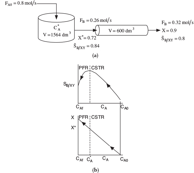
Figure E8-1.2 Effect of adding a PFR to increase conversion, (a) Reactor arrangement; (b) Selectivity and conversion trajectories.

This calculation for the PFR is carried out in the Chapter 8 Expanded Material on the CRE Web site (http://www.umich.edu/~elements/5e/08chap/expanded.html). The results of this calculation show that at the exit of the PFR, the molar flow rates are F_x = 0.22 mol/s, F_B = 0.32 mol/s, and F_Y = 0.18 mol/s corresponding to a conversion of X = 0.9. The corresponding selectivity at a conversion of 90% is

Do you really want to add the PFR?

${\tilde{S}}_{B/XY} = \frac{F_{B}}{F_{X} + F_{Y}} = 0.8$ ${\tilde{S}}_{B/XY} = \frac{F_{B}}{F_{X} + F_{Y}} = 0.8$

Analysis: One now has to make a decision as to whether adding the PFR to increase the conversion of A from 0.72 to 0.9 and the molar flow rate of the desired product B from 0.26 to 0.32 mol/s is worth not only the added cost of the PFR, but also the decrease in selectivity from 0.84 to 0.8. In this example, we used the Tram-bouze reactions to show how to optimize the selectivity to species B in a CSTR. Here, we found the optimal exit conditions (C_A = 0.112 mol/dm³), conversion (X = 0.72), and selectivity (S_B/_XY = 0.84). The corresponding CSTR volume was V = 1564 dm³. If we wanted to increase the conversion to 90%, we could use a PFR to follow the CSTR, but we would find that the selectivity decreased.

8.3.3 Reactor Selection and Operating Conditions

Next, consider two simultaneous reactions in which two reactants, A and B, are being consumed to produce a desired product, D, and an unwanted product, U, resulting from a side reaction. The rate laws for the reactions

\begin{matrix} A + B \overset{k_{1}}{\to} D \\ A + B \overset{k_{2}}{\to} U \end{matrix}

$\begin{matrix} A + B \overset{k_{1}}{\to} D \\ A + B \overset{k_{2}}{\to} U \end{matrix}$

are

\begin{matrix} r_{D} = k_{1} C_{A}^{α_{1}} C_{B}^{β_{1}} & (8-14) \end{matrix}

$\begin{matrix} r_{D} = k_{1} C_{A}^{α_{1}} C_{B}^{β_{1}} & (8-14) \end{matrix}$

\begin{matrix} r_{U} = k_{2} C_{A}^{α_{2}} C_{B}^{β_{2}} & (8-15) \end{matrix}

$\begin{matrix} r_{U} = k_{2} C_{A}^{α_{2}} C_{B}^{β_{2}} & (8-15) \end{matrix}$

The instantaneous selectivity

Instantaneous selectivity

$\begin{matrix} S_{D / U} = \frac{r_{D}}{r_{U}} = \frac{k_{1}}{k_{2}} C_{A}^{α_{1} - α_{2}} C_{B}^{β_{1} - β_{2}} & (8 - 16) \end{matrix}$ $\begin{matrix} S_{D / U} = \frac{r_{D}}{r_{U}} = \frac{k_{1}}{k_{2}} C_{A}^{α_{1} - α_{2}} C_{B}^{β_{1} - β_{2}} & (8 - 16) \end{matrix}$

is to be maximized. Shown in Figure 8-2 are various reactor schemes and conditions that might be used to maximize S_Oj_V.

The two reactors with recycle shown in (i) and 0) can also be used for highly exothermic reactions. Here, the recycle stream is cooled and returned to the reactor to dilute and cool the inlet stream, thereby avoiding hot spots and runaway reactions. The PFR with recycle is used for gas-phase reactions, and the CSTR is used for liquid-phase reactions.

Cartoon shows gas coming out of a reactor and a person scared of the gas running in full speed.

The last two reactors in Figure 8-2, (k) and (1), are used for thermodynam-ically limited reactions where the equilibrium lies far to the left (reactant side)

A + B ⇆ C + D

$A + B ⇆ C + D$

and one of the products must be removed (e.g., C) for the reaction to continue to completion. The membrane reactor (k) is used for thermodynamically limited gas-phase reactions, while reactive distillation (1) is used for liquid-phase reactions when one of the products has a higher volatility (e.g., C) than the other species in the reactor.

In making our selection of a reactor, the criteria are safety, selectivity, yield, temperature control, and cost.

Twelve illustrations show different reactors.

Illustration (a) labeled "CSTR" shows two inlets, labeled A and B, at the top left of an equipment with blades partly filled with mixture. An outlet at the bottom right is labeled D AND U. Text to the left reads: Reactor schemes to improve selectivity. Illustration (b) labeled "tubular reactor" shows two rightward arrows labeled A and B at the left and a rightward arrow labeled D and U. Illustration (c) labeled "batch" shows an equipment with blades partly filled with mixture. Illustration (d) labeled "semi-batch" shows an equipment with blades partly filled with mixture labeled Pure A initially. An arrow passes through an inlet at the top left labeled B and a closed outlet at the top right is shown. Illustration (e) labeled "semi-batch" shows an equipment with blades partly filled with mixture labeled Pure B initially. An inlet at the top left labeled A and a closed outlet at the top right is shown. Illustration (f) labeled "membrane reactor or a tubular reactor with side streams" shows two rightward arrows labeled A and B at the left, a rightward arrow labeled D AND U, and four arrows from the bottom side. Illustration (g) labeled "membrane reactor or a tubular reactor with side streams" shows two rightward arrows labeled A and B at the left, a rightward arrow labeled D AND U, and four arrows from the top side. Illustration (h) labeled "Series of small CSTRs" shows three small CSTRs with two outlets at the top left and an outlet at the right. Arrows labeled B pass through the second inlet of each equipment. An arrow labeled A passes through the first inlet of the first equipment with blades partly filled with a mixture. An outlet at the right of the first container is connected to the first inlet of the second equipment. An outlet at the right is connected to the first inlet of the third equipment. An outlet at the right is labeled D and U. Illustration (i) labeled "Tubular reactor with recycle" shows an equipment with blades partly filled with a mixture. Two arrows labeled A and B linked to the left and a rightward arrow labeled D and U. From the right, a leftward arrow with a squatter's symbol connects to the second inlet at the top left. Illustration (j) labeled "CSTR with recycle" shows arrows from A and B connected to the first inlet and an outlet labeled D AND U from the outlet. From the right, a leftward arrow with a squatter's symbol connects to the second inlet at the top left. Illustration (k) labeled "membrane reactor" shows two arrows labeled A and B linked to the left and a rightward arrow labeled D AND U. Arrows from the reactor, toward the sides are labeled C. Illustration (l) labeled "Reactive distillation" shows arrows from A and B connected to the first inlet and an outlet labeled D AND U from the outlet. An upward arrow from the second inlet is labeled C.

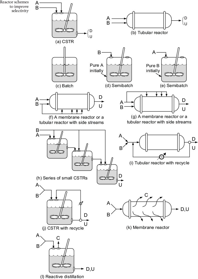
Figure 8-2 Different reactors and schemes for maximizing S_D|u in Equation 8-16. Note unreacted A and B also exit the reactor along with D and U.

Reactor Selection

Criteria:

• Safety

• Selectivity

• Yield

• Temperature control

• Cost

Example 8-2 Chowe of Reactor and Conditions to Minimize Unwanted Products

For the parallel reactions

\begin{matrix} A + B \to D: & r_{D} = k_{1} C_{A}^{α_{1}} C_{B}^{β_{1}} \\ A + B \to U : & r_{U} = k_{2} C_{A}^{α_{2}} C_{B}^{β_{2}} \end{matrix}

$\begin{matrix} A + B \to D: & r_{D} = k_{1} C_{A}^{α_{1}} C_{B}^{β_{1}} \\ A + B \to U : & r_{U} = k_{2} C_{A}^{α_{2}} C_{B}^{β_{2}} \end{matrix}$

consider all possible combinations of reaction orders and select the reaction scheme that will maximize S_D/_U .

Solution

Case 1: α₁ > α₂, β₁ > β₂ . Let a = α₁ — α₂ and b = β₁ — β₂ , where a and b are positive constants. Using these definitions, we can write Equation (8-16) in the form

$\begin{matrix} S_{D/U} = \frac{r_{D}}{r_{U}} = \frac{k_{1}}{k_{2}} C_{A}^{a} C_{B}^{b} & (E8-2 .1) \end{matrix}$ $\begin{matrix} S_{D/U} = \frac{r_{D}}{r_{U}} = \frac{k_{1}}{k_{2}} C_{A}^{a} C_{B}^{b} & (E8-2 .1) \end{matrix}$

To maximize the ratio r_O/r_v, maintain the concentrations of both A and B as high as possible. To do this, use

• A tubular reactor, Figure 8-2 (b).

• A batch reactor, Figure 8-2(c).

• High pressures (if gas phase), and reduce inerts.

Case 2: α₁ > α₂ , β₁ < β₂ . Let a = α₁ — α₂ and b = β₂ — β₁, where a and b are positive constants. Using these definitions, we can write Equation (8-16) in the form

\begin{matrix} S_{D/U} = \frac{r_{D}}{r_{U}} = \frac{k_{1} C_{A}^{a}}{k_{2} C_{B}^{b}} & (E8-2.2) \end{matrix}

$\begin{matrix} S_{D/U} = \frac{r_{D}}{r_{U}} = \frac{k_{1} C_{A}^{a}}{k_{2} C_{B}^{b}} & (E8-2.2) \end{matrix}$

To make S_D/_U as large as possible, we want to make the concentration of A high and the concentration of B low. To achieve this result, use

• A semibatch reactor in which B is fed slowly into a large amount of A as in Figure 8-2 (d).

• A membrane reactor or a tubular reactor with side streams of B continually fed to the reactor as in Figure 8-2 (f).

• A series of small CSTRs with A fed only to the first reactor and small amounts of B fed to each reactor. In this way, B is mostly consumed before the CSTR exit stream flows into the next reactor as in Figure 8-2(h).

Case 3: α₁ < α₂ , β₁ < β₂ . Let a = α₂ — α₁ and b = β₂ — β₁, where a and b are positive constants. Using these definitions, we can write Equation (8-16) in the form

\begin{matrix} S_{D/U} = \frac{r_{D}}{r_{U}} = \frac{k_{1}}{k_{2} C_{A}^{a} C_{B}^{b}} & (E8-2.3) \end{matrix}

$\begin{matrix} S_{D/U} = \frac{r_{D}}{r_{U}} = \frac{k_{1}}{k_{2} C_{A}^{a} C_{B}^{b}} & (E8-2.3) \end{matrix}$

To make S_D/U as large as possible, the reaction should be carried out at low concentrations of A and of B. Use

• A CSTR as in Figure 8-2(a).

• A tubular reactor in which there is a large recycle ratio as in Figure 8-2(i).

• A feed diluted with inerts.

• Low pressure (if gas phase).

Case 4: α₁< α₂ , β₁ > β₂. Let a = α₂ — α₁ and b = ß₁ — β₂, where a and b are positive constants. Using these definitions, we can write Equation (8-16) in the form

\begin{matrix} S_{D/U} = \frac{r_{D}}{r_{U}} = \frac{k_{1} C_{B}^{b}}{k_{2} C_{A}^{a}} & (E8-2.4) \end{matrix}

$\begin{matrix} S_{D/U} = \frac{r_{D}}{r_{U}} = \frac{k_{1} C_{B}^{b}}{k_{2} C_{A}^{a}} & (E8-2.4) \end{matrix}$

To maximize S_D/U, run the reaction at high concentrations of B and low concentrations of A. Use

• A semibatch reactor with A slowly fed to a large amount of B as in Figure 8-2(e).

• A membrane reactor or a tubular reactor with side streams of A as in Figure 8-2 (g).

• A series of small CSTRs with fresh A fed to each reactor.

Analysis: In this very important example we showed how to use the instantaneous selectivity, S_D_/_U, to guide the initial selection of the type of reactor and reactor system to maximize the selectivity with respect to the desired species D. The final selection should be made after one calculates the overall selectivity ${\tilde{S}}_{D/U}$ ${\tilde{S}}_{D/U}$ for the reactors and operating conditions chosen.

8.4 Reactions in Series

In Section 8.1, we saw that the undesired product could be minimized by adjusting the reaction conditions (e.g., concentration, temperature) and by choosing the proper reactor. For series (i.e., consecutive) reactions, the most important variable is time: space time for a flow reactor and real time for a batch reactor. To illustrate the importance of the time factor, we consider the sequence

Graph shows the horizontal axis represents t and the vertical axis represents C subscript i. A bell-shaped curve labeled "B." Two curves labeled "A and B" intersect the bell curve.

A \overset{k_{1}}{\to} B \overset{k_{2}}{\to} C

$A \overset{k_{1}}{\to} B \overset{k_{2}}{\to} C$

in which species B is the desired product.

If the first reaction is slow and the second reaction is fast, it will be extremely difficult to produce a significant amount of species B. If the first reaction (formation of B) is fast and the reaction to form C is slow, a large yield of B can be achieved. However, if the reaction is allowed to proceed for a long time in a batch reactor, or if the tubular flow reactor is too long, the desired product B will be converted to the undesired product C. In no other type of reaction is exactness in the calculation of the time needed to carry out the reaction more important than in series reactions.

Example 8-3 Series Reactions in a Batch Reactor

The elementary liquid-phase series reaction

A \overset{k_{1}}{\to} B \overset{k_{2}}{\to} C

$A \overset{k_{1}}{\to} B \overset{k_{2}}{\to} C$

is carried out in a batch reactor. The reaction is heated very rapidly to the reaction temperature, where it is held at this temperature until the time it is quenched by rapidly lowering the temperature.

(a) Plot and analyze the concentrations of species A, B, and C as a function of time.

(b) Calculate the time to quench the reaction when the concentration of B will be a maximum.

Additional Information

C_A0 = 2M, k₁=0.5h^-1, k₂ =0.2h^-1

Solution

Part (a)

0. Number the Reactions:

The preceding series reaction can be written as two reactions

\begin{matrix} (1) Reaction 1 & A \overset{k_{1}}{\to} B & - r_{1 A} = k_{1} C_{A} \\ (2) Reaction 2 & A \overset{k_{2}}{\to} C & - r_{2B} = k_{2} C_{B} \end{matrix}

$\begin{matrix} (1) Reaction 1 & A \overset{k_{1}}{\to} B & - r_{1 A} = k_{1} C_{A} \\ (2) Reaction 2 & A \overset{k_{2}}{\to} C & - r_{2B} = k_{2} C_{B} \end{matrix}$

1. Mole Balances:

1A. Mole Balance on A:

\frac{d N_{A}}{dt} = r_{A} V

$\frac{d N_{A}}{dt} = r_{A} V$

a. Mole balance in terms of concentration for V = V₀ becomes

\begin{matrix} \frac{d C_{A}}{dt} = r_{A} & (E8-3.1) \end{matrix}

$\begin{matrix} \frac{d C_{A}}{dt} = r_{A} & (E8-3.1) \end{matrix}$

b. Rate law for Reaction 1: Reaction is elementary

\begin{matrix} r_{A} = r_{1 A} = - k_{1} C_{A} & (E8-3.2) \end{matrix}

$\begin{matrix} r_{A} = r_{1 A} = - k_{1} C_{A} & (E8-3.2) \end{matrix}$

c. Combining the mole balance and rate law

\begin{matrix} \frac{{dC}_{_{A}}}{dt} = - k_{1} C_{A} & (E8-3.3) \end{matrix}

$\begin{matrix} \frac{{dC}_{_{A}}}{dt} = - k_{1} C_{A} & (E8-3.3) \end{matrix}$

Integrating with the initial condition C_A = C_A0 at t = 0

\begin{matrix} In \frac{C_{_{A}}}{C_{A0}} = - k_{1} t & (E8-3.4) \end{matrix}

$\begin{matrix} In \frac{C_{_{A}}}{C_{A0}} = - k_{1} t & (E8-3.4) \end{matrix}$

Solving for C_A

$\begin{matrix} C_{A} = C_{A0} e^{- k_{1} t} & (E8-3 .5) \end{matrix}$ $\begin{matrix} C_{A} = C_{A0} e^{- k_{1} t} & (E8-3 .5) \end{matrix}$

IB. Mole Balance on B:

a. Mole balance for a constant-volume batch reactor becomes

\begin{matrix} \frac{{dC}_{B}}{dt} = r_{B} & (E8-3.6) \end{matrix}

$\begin{matrix} \frac{{dC}_{B}}{dt} = r_{B} & (E8-3.6) \end{matrix}$

b. Rates:

Rate Laws

Elementary reactions

\begin{matrix} r_{2 B} = - k_{2} C_{B} & (E8-3.7) \end{matrix}

$\begin{matrix} r_{2 B} = - k_{2} C_{B} & (E8-3.7) \end{matrix}$

Relative Rates

Rate of formation of B in Reaction 1 equals the rate of disappearance of A in Reaction 1.

\begin{matrix} r_{1B} = - r_{1 A} = k_{1} C_{A} & (E8-3.8) \end{matrix}

$\begin{matrix} r_{1B} = - r_{1 A} = k_{1} C_{A} & (E8-3.8) \end{matrix}$

Net Rates

The net rate of reaction of B will be the rate of formation of B in reaction (1) plus the rate of formation of B in reaction (2).

\begin{matrix} r_{B} = r_{1 B} + r_{2 B} & (E8-3.9) \end{matrix}

$\begin{matrix} r_{B} = r_{1 B} + r_{2 B} & (E8-3.9) \end{matrix}$

\begin{matrix} r_{B} = k_{1} C_{A} - k_{2} C_{B} & (E8-3.10) \end{matrix}

$\begin{matrix} r_{B} = k_{1} C_{A} - k_{2} C_{B} & (E8-3.10) \end{matrix}$

c. Combining the mole balance and rate law

\begin{matrix} \frac{{dC}_{B}}{dt} = k_{1} C_{A} - k_{2} C_{B} & (E8-3.11) \end{matrix}

$\begin{matrix} \frac{{dC}_{B}}{dt} = k_{1} C_{A} - k_{2} C_{B} & (E8-3.11) \end{matrix}$

Rearranging and substituting for C_A

\begin{matrix} \frac{{dC}_{B}}{dt} + k_{2} C_{B} = k_{1} C_{{A0}^{e}} - k_{1} t & (E8-3.12) \end{matrix}

$\begin{matrix} \frac{{dC}_{B}}{dt} + k_{2} C_{B} = k_{1} C_{{A0}^{e}} - k_{1} t & (E8-3.12) \end{matrix}$

Using the integrating factor gives

There is a tutorial on the integrating factor in Appendix A and on the CRE Web site.

\begin{matrix} \frac{d ({C_{B^{e}}}^{k_{2} t})}{dt} = k_{1} {C_{{A0}^{e}}}^{(k_{2} - k_{1}) t} & (E8-3.13) \end{matrix}

$\begin{matrix} \frac{d ({C_{B^{e}}}^{k_{2} t})}{dt} = k_{1} {C_{{A0}^{e}}}^{(k_{2} - k_{1}) t} & (E8-3.13) \end{matrix}$

At time t = 0, C_B = 0. Solving Equation (E8-3.13) gives

$\begin{matrix} C_{B} = k_{1} C_{A0} [\frac{e^{- k_{1} t} - e^{- k_{2} t}}{k_{2} - k_{1}}] & (E8-3 .14) \end{matrix}$ $\begin{matrix} C_{B} = k_{1} C_{A0} [\frac{e^{- k_{1} t} - e^{- k_{2} t}}{k_{2} - k_{1}}] & (E8-3 .14) \end{matrix}$

1C. Mole Balance on C:

The mole balance on C is similar to Equation (E8-3.1).

\begin{matrix} \frac{{dC}_{c}}{dt} = r_{c} & (E8-3.15) \end{matrix}

$\begin{matrix} \frac{{dC}_{c}}{dt} = r_{c} & (E8-3.15) \end{matrix}$

The rate of formation of C is just the rate of disappearance of B in reaction (2), i.e., r_c = -r_2B = k₂C_B

\begin{matrix} \frac{{dC}_{c}}{dt} = k_{2} C_{B} & (E8-3.16) \end{matrix}

$\begin{matrix} \frac{{dC}_{c}}{dt} = k_{2} C_{B} & (E8-3.16) \end{matrix}$

Substituting for C_B

\begin{matrix} \frac{{dC}_{c}}{dt} = \end{matrix} \frac{k_{1} k_{2} C_{A0}}{k_{2} - k_{1}} (e^{- k_{1} t} - e^{- k_{2} t})

$\begin{matrix} \frac{{dC}_{c}}{dt} = \end{matrix} \frac{k_{1} k_{2} C_{A0}}{k_{2} - k_{1}} (e^{- k_{1} t} - e^{- k_{2} t})$

and integrating with C_c = 0 at t = 0 gives

$\begin{matrix} C_{C} = \frac{C_{A0}}{k_{2} - k_{1}} [k_{2} [1 - e^{- k_{1} t}] - k_{1} [1 - e^{- k_{2} t}]] & (E8-3 .17) \end{matrix}$ $\begin{matrix} C_{C} = \frac{C_{A0}}{k_{2} - k_{1}} [k_{2} [1 - e^{- k_{1} t}] - k_{1} [1 - e^{- k_{2} t}]] & (E8-3 .17) \end{matrix}$

Note that as t —>∞ then C_c = C_A0 as expected. We also note the concentration of C, C_c, could have been obtained more easily from an overall balance.

Calculating the concentration of C the easy way

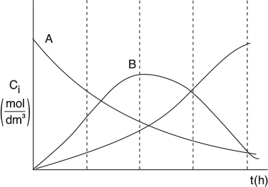
$\begin{matrix} C_{C} = C_{A0} - C_{A} - C_{B} & (E8-3 .18) \end{matrix}$ $\begin{matrix} C_{C} = C_{A0} - C_{A} - C_{B} & (E8-3 .18) \end{matrix}$

The concentrations of A, B, and C are shown as a function of time in Figure E8-3.1.

Graph shows the horizontal axis represents "t (in height)" and the vertical axis represents "C subscript i (in moles per cubic decimeter)." A bell-shaped curve labeled "B." Two curves labeled "A and B" intersect the bell curve. Four vertical dashed lines are also shown.

Figure E8-3.1 Concentration trajectories in a batch reactor.

Part (b)

1. Concentration and Time at the Maximum

We note from Figure E8-3.1 that the concentration of B goes through a maximum. Consequently, to find the maximum we need to differentiate Equation E8-3.14 and set it to zero.

\begin{matrix} \begin{matrix} \frac{{dC}_{B}}{dt} = 0 = \end{matrix} \frac{k_{1} C_{A0}}{k_{2} - k_{1}} [- k_{1} e^{- k_{1} t} + k_{2} e^{- k_{2} t}] & (E8-3.19) \end{matrix}

$\begin{matrix} \begin{matrix} \frac{{dC}_{B}}{dt} = 0 = \end{matrix} \frac{k_{1} C_{A0}}{k_{2} - k_{1}} [- k_{1} e^{- k_{1} t} + k_{2} e^{- k_{2} t}] & (E8-3.19) \end{matrix}$

Solving for t_max gives

$\begin{matrix} t_{\max} = \frac{1}{k_{2} - k_{1}} In \frac{k_{2}}{k_{1}} & (E8-3 .20) \end{matrix}$ $\begin{matrix} t_{\max} = \frac{1}{k_{2} - k_{1}} In \frac{k_{2}}{k_{1}} & (E8-3 .20) \end{matrix}$

Substituting Equation (E8-3.20) into Equation (E8-3.5), we find the concentration of A at the maximum for C_R is

Series Reaction

\begin{matrix} C_{A} = {C_{{A0}^{e}}}^{- k_{1} (\frac{1}{k_{2} - k_{1}} in \frac{k_{2}}{k_{1}})} & (E8-3.21) \end{matrix}

$\begin{matrix} C_{A} = {C_{{A0}^{e}}}^{- k_{1} (\frac{1}{k_{2} - k_{1}} in \frac{k_{2}}{k_{1}})} & (E8-3.21) \end{matrix}$

$\begin{matrix} C_{A} = C_{A0} {[\frac{k_{1}}{k_{2}}]}^{\frac{k_{1}}{k_{2} - k_{1}}} & (E8-3 .22) \end{matrix}$ $\begin{matrix} C_{A} = C_{A0} {[\frac{k_{1}}{k_{2}}]}^{\frac{k_{1}}{k_{2} - k_{1}}} & (E8-3 .22) \end{matrix}$

Similarly, the concentration of B at the maximum is

$\begin{matrix} C_{B} = \frac{k_{1} C_{A0}}{k_{2} - k_{1}} [{(\frac{k_{1}}{k_{2}})}^{^{\frac{k_{1}}{k_{2} - k_{1}}}} - {(\frac{k_{1}}{k_{2}})}^{^{\frac{k_{2}}{k_{2} - k_{1}}}}] & (E8-3 .23) \end{matrix}$ $\begin{matrix} C_{B} = \frac{k_{1} C_{A0}}{k_{2} - k_{1}} [{(\frac{k_{1}}{k_{2}})}^{^{\frac{k_{1}}{k_{2} - k_{1}}}} - {(\frac{k_{1}}{k_{2}})}^{^{\frac{k_{2}}{k_{2} - k_{1}}}}] & (E8-3 .23) \end{matrix}$

2. Evaluate: Substituting for C_A0 = 2 mol/dm³, k₁ = 0.5h^-1, and k₂ ⁼ 0.2h^-1 in Equations (E8-3.5), (E8-3.14), and (E8-3.18), the concentrations as a function of time are

\begin{matrix} C_{A} = 2 mol / {dm}^{3} (e^{- 0.5 t}) \\ C_{B} = \frac{2 (mol / {dm}^{3})}{(0.2–0.5)} (0.5) (e^{- 0.5 t} - e^{- 0.2 t}) \\ C_{B} = 3.33 (mol / {dm}^{3}) [e^{- 0.2 t} - e^{- 0.5 t}] \\ C_{c} = 2 mol / {dm}^{3} - 2 (mol / {dm}^{3}) e^{- 0.5 t} - 3.33 {mol/dm}^{3} [e^{- 0.2 t} - e^{- 0.5 t}] \end{matrix}

$\begin{matrix} C_{A} = 2 mol / {dm}^{3} (e^{- 0.5 t}) \\ C_{B} = \frac{2 (mol / {dm}^{3})}{(0.2–0.5)} (0.5) (e^{- 0.5 t} - e^{- 0.2 t}) \\ C_{B} = 3.33 (mol / {dm}^{3}) [e^{- 0.2 t} - e^{- 0.5 t}] \\ C_{c} = 2 mol / {dm}^{3} - 2 (mol / {dm}^{3}) e^{- 0.5 t} - 3.33 {mol/dm}^{3} [e^{- 0.2 t} - e^{- 0.5 t}] \end{matrix}$

Substituting in Equation (E8-3.20)

t_{max} = \frac{1}{0.2–0.5} in \frac{0.2}{0.5} = \frac{1}{0.3} in \frac{0.5}{0.2}

$t_{max} = \frac{1}{0.2–0.5} in \frac{0.2}{0.5} = \frac{1}{0.3} in \frac{0.5}{0.2}$

$\begin{matrix} t_{max} = 3.05 h \end{matrix}$ $\begin{matrix} t_{max} = 3.05 h \end{matrix}$

The time to quench the reaction is at 3.05 h.

At t_max = 3.05 h, the concentrations of A, B, and C are

\begin{matrix} C_{A} = 2 \frac{mol}{{dm}^{3}} [(\frac{0.5}{0.2})^{(\frac{(0.5)}{0.2–0.5})}] = 0.43 \frac{mol}{{dm}^{3}} \\ C_{B} = 2 \frac{mol (0.5)}{{dm}^{3} (0.2–0.5)} [(\frac{0.5}{0.2})^{(\frac{(0.5)}{0.2–0.5})} - (\frac{0.5}{0.2})^{(\frac{0.2}{0.2–0.5})}] \\ C_{B} = 1.09 \frac{mol}{{dm}^{3}} \end{matrix}

$\begin{matrix} C_{A} = 2 \frac{mol}{{dm}^{3}} [(\frac{0.5}{0.2})^{(\frac{(0.5)}{0.2–0.5})}] = 0.43 \frac{mol}{{dm}^{3}} \\ C_{B} = 2 \frac{mol (0.5)}{{dm}^{3} (0.2–0.5)} [(\frac{0.5}{0.2})^{(\frac{(0.5)}{0.2–0.5})} - (\frac{0.5}{0.2})^{(\frac{0.2}{0.2–0.5})}] \\ C_{B} = 1.09 \frac{mol}{{dm}^{3}} \end{matrix}$

The concentration of C at the time we quench the reaction is

C_c = C_A0 - C_A - C_B = 2 - 0.44 - 1.07 = 0.48 mol/dm³

Part (c) Calculate the overall selectivity and yield at the reaction quench time. The selectivity is

S_{B/ C} = \frac{C_{B}}{C_{C}} = \frac{1.09}{0.48} = 2.3

$S_{B/ C} = \frac{C_{B}}{C_{C}} = \frac{1.09}{0.48} = 2.3$

The yield is

Y_{B} = \frac{C_{B}}{C_{A0} - C_{A}} = \frac{1.09}{2–0.48} = 0.69

$Y_{B} = \frac{C_{B}}{C_{A0} - C_{A}} = \frac{1.09}{2–0.48} = 0.69$

Analysis: In this example, we applied our CRE algorithm for multiple reactions to the series reaction A —> B —> C. Here, we obtained an analytical solution to find the time at which the concentration of the desired product B was a maximum and, consequently, the time to quench the reaction. We also calculated the concentrations of A, B, and C at this time, along with the selectivity and yield.

We will now carry out this same series reaction in a CSTR.

Example 8-4 Series Reaction in a CSTR

The reactions discussed in Example 8-3 are now to be carried out in a CSTR.

\begin{matrix} A \overset{k_{1}}{\to} B \\ B \overset{k_{2}}{\to} C \end{matrix}

$\begin{matrix} A \overset{k_{1}}{\to} B \\ B \overset{k_{2}}{\to} C \end{matrix}$

(a) Determine the exit concentrations from the CSTR.

(b) Find the value of the space time τ that will maximize the concentration of B.

Solution

Part (a)

1. a. Mole Balance on A:

IN	-	OUT	+	GENERATION	=
F_A0	-	F_A	+	r_AV	=
u⁰ C^A0	-	v₀ C^A	+	r_A V	=

Dividing by υ₀, rearranging and recalling that τ=ν/υ₀, we obtain

\begin{matrix} C_{A0} - C_{A} + r_{A} τ = 0 & (E8-4.1) \end{matrix}

$\begin{matrix} C_{A0} - C_{A} + r_{A} τ = 0 & (E8-4.1) \end{matrix}$

b. Rates

The laws and net rates are the same as in Example 8-3.

\begin{matrix} Reaction 1: & r_{A} = - k_{1} C_{A} & (E8-4.2) \end{matrix}

$\begin{matrix} Reaction 1: & r_{A} = - k_{1} C_{A} & (E8-4.2) \end{matrix}$

C. Combining the mole balance of A with the rate of disappearance of A

\begin{matrix} C_{A0} - C_{A} - k_{1} C_{A} τ = 0 & (E8-4.3) \end{matrix}

$\begin{matrix} C_{A0} - C_{A} - k_{1} C_{A} τ = 0 & (E8-4.3) \end{matrix}$

Solving for C_A

$\begin{matrix} C_{A} = \frac{C_{A0}}{1 + τ k_{1}} & (E8-4 .4) \end{matrix}$ $\begin{matrix} C_{A} = \frac{C_{A0}}{1 + τ k_{1}} & (E8-4 .4) \end{matrix}$

We now use the same algorithm for species B we did for species A to solve for the concentration of B.

2. a. Mole Balance on B:

IN	-	OUT	+	GENERATION	=
0	-	F_b	+	r_BV	=
	-	v₀ C_B	+	r_BV	=

Dividing by v₀ and rearranging

\begin{matrix} - C_{B} + r_{B} τ = 0 & (E8-4.5) \end{matrix}

$\begin{matrix} - C_{B} + r_{B} τ = 0 & (E8-4.5) \end{matrix}$

b. Rates

The laws and net rates are the same as in Example 8-3.

Net Rates

\begin{matrix} r_{_{B}} = k_{1} C_{A} - k_{2} C_{B} & (E8-4.6) \end{matrix}

$\begin{matrix} r_{_{B}} = k_{1} C_{A} - k_{2} C_{B} & (E8-4.6) \end{matrix}$

c. Combine

- C_{B} + (k_{1} C_{A} - k_{2} C_{B}) τ = 0

$- C_{B} + (k_{1} C_{A} - k_{2} C_{B}) τ = 0$

\begin{matrix} C_{B} = \frac{k_{1} C_{A} τ}{1 + k_{2} τ} & (E8-4.7) \end{matrix}

$\begin{matrix} C_{B} = \frac{k_{1} C_{A} τ}{1 + k_{2} τ} & (E8-4.7) \end{matrix}$

Substituting for C_A

$\begin{matrix} C_{B} = \frac{τ k_{1} C_{A0}}{(1 + k_{1} τ) (1 + k_{2} τ)} & (E8-4 .8) \end{matrix}$ $\begin{matrix} C_{B} = \frac{τ k_{1} C_{A0}}{(1 + k_{1} τ) (1 + k_{2} τ)} & (E8-4 .8) \end{matrix}$

3. Mole Balance on C:

\begin{matrix} 0 - ν_{0} C_{C} + r_{C} V = 0 \\ - C_{C} + r_{C} τ = 0 & (E8-4.9) \end{matrix}

$\begin{matrix} 0 - ν_{0} C_{C} + r_{C} V = 0 \\ - C_{C} + r_{C} τ = 0 & (E8-4.9) \end{matrix}$

Rates

\begin{matrix} r_{c} = - r_{2 B} = k_{2} C_{B} \\ C_{C} = r_{C} τ = k_{2} C_{B} τ \end{matrix}

$\begin{matrix} r_{c} = - r_{2 B} = k_{2} C_{B} \\ C_{C} = r_{C} τ = k_{2} C_{B} τ \end{matrix}$

$\begin{matrix} C_{C} = \frac{τ^{2} k_{1} k_{2} C_{A0}}{(1 + k_{1} τ) (1 + k_{2} τ)} & (E8-4 .10) \end{matrix}$ $\begin{matrix} C_{C} = \frac{τ^{2} k_{1} k_{2} C_{A0}}{(1 + k_{1} τ) (1 + k_{2} τ)} & (E8-4 .10) \end{matrix}$

Part (b) Optimum Concentration of B

To find the maximum concentration of B, we set the differential of Equation (E8-4.8) with respect to τ equal to zero

\frac{{dC}_{B}}{dτ} = \frac{k_{1} C_{A0} (1 + {τk}_{1}) (1 + {τk}_{2}) - {τk}_{1} C_{A0} (k_{1} + k_{2} + 2 {τk}_{1} k_{2})}{[(1 + k_{1} τ) (1 + k_{2} τ)]^{2}} = 0

$\frac{{dC}_{B}}{dτ} = \frac{k_{1} C_{A0} (1 + {τk}_{1}) (1 + {τk}_{2}) - {τk}_{1} C_{A0} (k_{1} + k_{2} + 2 {τk}_{1} k_{2})}{[(1 + k_{1} τ) (1 + k_{2} τ)]^{2}} = 0$

Solving for τ at which the concentration of B is a maximum at

$\begin{matrix} τ_{\max} = \frac{1}{\sqrt{k_{1} k_{2}}} & (E8-4 .11) \end{matrix}$ $\begin{matrix} τ_{\max} = \frac{1}{\sqrt{k_{1} k_{2}}} & (E8-4 .11) \end{matrix}$

The exiting concentration of B at the optimum value of τ is

\begin{matrix} C_{_{B}} = \frac{τ_{\max} k_{1} C_{A 0}}{(1 + τ_{\max} k_{1}) (1 + τ_{\max} k_{2})} = \frac{τ_{\max} k_{1} C_{A 0}}{1 + τ_{\max} k_{1} + τ_{\max} k_{2} + τ_{\max}^{2} k_{1} k_{2})} & (E8-4.12) \end{matrix}

$\begin{matrix} C_{_{B}} = \frac{τ_{\max} k_{1} C_{A 0}}{(1 + τ_{\max} k_{1}) (1 + τ_{\max} k_{2})} = \frac{τ_{\max} k_{1} C_{A 0}}{1 + τ_{\max} k_{1} + τ_{\max} k_{2} + τ_{\max}^{2} k_{1} k_{2})} & (E8-4.12) \end{matrix}$

Substituting Equation (E8-4.11) for τ_max in Equation (E8-4.12)

\begin{matrix} C_{B} = \frac{C_{A0} \frac{k_{1}}{\sqrt{k_{1} k_{2}}}}{1 + \frac{k_{1}}{\sqrt{k_{1} k_{2}}} + \frac{k_{2}}{\sqrt{k_{1} k_{2}}} + 1} & (E8-4.13) \end{matrix}

$\begin{matrix} C_{B} = \frac{C_{A0} \frac{k_{1}}{\sqrt{k_{1} k_{2}}}}{1 + \frac{k_{1}}{\sqrt{k_{1} k_{2}}} + \frac{k_{2}}{\sqrt{k_{1} k_{2}}} + 1} & (E8-4.13) \end{matrix}$

Rearranging, we find the concentration of B at the optimum space time is

$\begin{matrix} C_{B} = \frac{C_{A0} k_{1}}{2 \sqrt{k_{1} k_{2}} + k_{1} + k_{2}} & (E8-4 .14) \end{matrix}$ $\begin{matrix} C_{B} = \frac{C_{A0} k_{1}}{2 \sqrt{k_{1} k_{2}} + k_{1} + k_{2}} & (E8-4 .14) \end{matrix}$

Evaluation

τ_{\max} = \frac{1}{\sqrt{(0.5) (0.2)}} = 3.16 h

$τ_{\max} = \frac{1}{\sqrt{(0.5) (0.2)}} = 3.16 h$

At τ_max, the concentrations of A, B, and C are

C_{A} = \frac{C_{A0}}{1 + τ_{\max} k_{1}} = \frac{2 \frac{mol}{{dm}^{3}}}{1 + (3.16 h) (\frac{0.5}{h})} = 0.78 \frac{mol}{{dm}^{3}}

$C_{A} = \frac{C_{A0}}{1 + τ_{\max} k_{1}} = \frac{2 \frac{mol}{{dm}^{3}}}{1 + (3.16 h) (\frac{0.5}{h})} = 0.78 \frac{mol}{{dm}^{3}}$

C_{B} = 2 \frac{mol}{{dm}^{3}} \frac{0.5}{2 \sqrt{(0.2) (0.5)} + 0.2 + 0.5} = 0.75 \frac{mol}{{dm}^{3}}

$C_{B} = 2 \frac{mol}{{dm}^{3}} \frac{0.5}{2 \sqrt{(0.2) (0.5)} + 0.2 + 0.5} = 0.75 \frac{mol}{{dm}^{3}}$

C_{C} = C_{A0} - C_{A} - C_{B} = (2–0.78–0.75 \frac{mol}{{dm}^{3}}) = 0.47 \frac{mol}{{dm}^{3}}

$C_{C} = C_{A0} - C_{A} - C_{B} = (2–0.78–0.75 \frac{mol}{{dm}^{3}}) = 0.47 \frac{mol}{{dm}^{3}}$

The conversion is

X = \frac{C_{A0} - C_{A}}{C_{A0}} = \frac{2–0.78}{2} = 0.61

$X = \frac{C_{A0} - C_{A}}{C_{A0}} = \frac{2–0.78}{2} = 0.61$

The selectivity is

S_{B/C} = \frac{C_{B}}{C_{C}} = \frac{0.75}{0.47} = 1.60

$S_{B/C} = \frac{C_{B}}{C_{C}} = \frac{0.75}{0.47} = 1.60$

The yield is

Y_{B} = \frac{C_{B}}{C_{A0} - C_{A}} = \frac{0.75}{2–0.78} = 0.61

$Y_{B} = \frac{C_{B}}{C_{A0} - C_{A}} = \frac{0.75}{2–0.78} = 0.61$

Real data compared with real theory.

SUMMARY TABLE

	Time	${\tilde{S}}_{B/C}$ ${\tilde{S}}_{B/C}$	${\tilde{Y}}_{B}$ ${\tilde{Y}}_{B}$
Batch	t_max = 3.05 h	2.3	0.69
CSTR	τ_max = 3.16 h	1.6	0.61

Analysts: The CRE algorithm for multiple reactions was applied to the series reaction A —» B —» C in a CSTR to find the CSTR space time necessary to maximize the concentration of B, i.e., τ = 3.16 h. The conversion at this space time is 61%, the selectivity, S_B/C , is 1.60, and the yield, Y"_B , is 0.63. The conversion and selectivity are less for the CSTR than those for the batch reactor at the time of quenching.

PFR

If the series reaction were carried out in a PFR, the results would essentially be those of a batch reactor where we replaced the time variable “t” with the space time, “τ". Data for the series reaction

Ethanol \overset{k_{1}}{\to} Aldehyde \overset{k_{2}}{\to} Products

$Ethanol \overset{k_{1}}{\to} Aldehyde \overset{k_{2}}{\to} Products$

is compared for different values of the specific reaction rates, k₁ and k₂, in Figure 8-3.

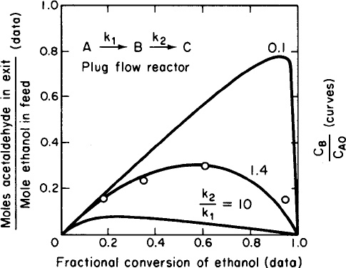
$Graph shows the fractional conversion of ethanol (data).$

Figure 8-3 Yield of acetaldehyde as a function of ethanol conversion. Data were obtained at 518 K. Data points (in order of increasing ethanol conversion) were obtained at space velocities of 26,000, 52,000,104,000, and 208,000 h^-1. The curves were calculated for a first-order series reaction in a plug-flow reactor and show yield of the intermediate species B as a function of the conversion of reactant for various ratios of rate constants k₂ and fe_a. (McCabe, Robert, W., and Patricia J. Mitchell. Oxidation of ethanol and acetaldehyde over alumina-supported catalysts. Industrial & Engineering Chemistry Product Research and Development 1983 22(2), 212-217. Copyright © 1963, American Chemical Society. Reprinted by permission.)

A complete analysis of this reaction carried out in a PFR is given on the CRE Web site.

Living Example Problem

Side Note: Blood Clotting

Many metabolic reactions involve a large number of sequential reactions, such as those that occur in the coagulation of blood.

Cut → Blood → Clotting

Blood coagulation (see Figure A) is part of an important host defense mechanism called hemostasis, which causes the cessation of blood loss from a damaged vessel. The clotting process is initiated when a nonenzymatic lipo-protein (called the tissue factor) contacts blood plasma because of cell damage. The tissue factor (TF) is normally not in contact with plasma (see Figure B) because of an intact endothelium. The rupture (e.g., cut) of the endothe-lium exposes the plasma to TF and a cascade* of series reactions proceeds (Figure C). These series reactions ultimately result in the conversion of fibrinogen (soluble) to fibrin (insoluble), which produces the clot. Later, as wound healing occurs, mechanisms that restrict formation of fibrin clots, necessary to maintain the fluidity of the blood, start working.

Ouch!

Photograph shows two vials of blood samples.

Figure A Normal clot coagulation of blood. (Dietrich Mebs, Venomous and Poisonous Animals, Stuttgart: Medpharm, (2002), p. 305. Reprinted by permission of the author.)

Plasma contacting tissue factor is depicted.

Figure B Schematic of separation of TF (A) and plasma (B) before cut occurs.

Figure C Cut allows contact of plasma to initiate coagulation. (A + B → Cascade)

* Platelets provide procoagulant, phospholipids-equivalent surfaces upon which the complex-dependent reactions of the blood coagulation cascade are localized.

An abbreviated form (1) of the initiation and following cascade metabolic reactions that can capture the clotting process is

Reaction involved in clotting process is shown.

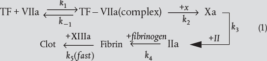
In order to maintain the fluidity of the blood, the clotting sequence (2) must be moderated. The reactions that attenuate the clotting process are

\begin{matrix} {ATIII+X}_{a} & \overset{k_{6}}{\to} & {Xa}_{inactive} \\ {ATIII+II}_{a} & \overset{k_{7}}{\to} & {IIa}_{inactive} & (2) \\ ATIII+TF-VII a & \overset{k_{8}}{\to} & {TF-VIIa}_{inactive} \end{matrix}

$\begin{matrix} {ATIII+X}_{a} & \overset{k_{6}}{\to} & {Xa}_{inactive} \\ {ATIII+II}_{a} & \overset{k_{7}}{\to} & {IIa}_{inactive} & (2) \\ ATIII+TF-VII a & \overset{k_{8}}{\to} & {TF-VIIa}_{inactive} \end{matrix}$

where TF = tissue factor, VIIa = factor novoseven, X = Stuart Prower factor, Xa = Stuart Prower factor activated, II = prothrombin, Ha = thrombin, ATIII = antithrombin, and XIIIa = factor XIIa.

Symbolically, the clotting equations can be written as

Cut → A + B → C → D → E → F → Clot

One can model the clotting process in a manner identical to the series reactions by writing a mole balance and rate law for each species, such as

\begin{matrix} \frac{{dC}_{TF}}{dt} = - k_{1} \cdot C_{TF} \cdot C_{VII a} + k_{- 1} \cdot C_{TF - VII a} \\ \frac{{dC}_{VIIa}}{dt} = - k_{1} \cdot C_{TF} \cdot C_{VII a} + k_{- 1} \cdot C_{TF - VII a} \end{matrix}

$\begin{matrix} \frac{{dC}_{TF}}{dt} = - k_{1} \cdot C_{TF} \cdot C_{VII a} + k_{- 1} \cdot C_{TF - VII a} \\ \frac{{dC}_{VIIa}}{dt} = - k_{1} \cdot C_{TF} \cdot C_{VII a} + k_{- 1} \cdot C_{TF - VII a} \end{matrix}$

etc.

The next time you have to go to the emergency room for a serious cut, discussing the clotting mechanism should impress the doctor as you are stitched up.

and then using Polymath to solve the coupled equations to predict the thrombin (shown in Figure D) and other species concentration as a function of time, as well as to determine the clotting time. Laboratory data are also shown below for a TF concentration of 5 pM. One notes that when the complete set of equations is used, the Polymath output is identical to Figure E. The complete set of equations, along with the Polymath Living Example Problem LEP code (http://www.umich.edu/~elements/5e/08chap/live.html) is given in the Solved Problems on the CRE Web site (http://www.umich.edu/~elements/5e/08chap/pdf/BloodCoagulation.pdf). You can load the program directly and vary some of the parameters.

Graph shows the total thrombin as a function of time for the abbreviated blood-clotting cascade.

Figure D Total thrombin as a function of time with an initiating TF concentration of 25 pM (after running Polymath) for the abbreviated blood-clotting cascade.

Graph shows the total thrombin as a function of time for the full blood clotting cascade.

Figure E Total thrombin as a function of time with an initiating TF concentration of 25 pM. Full blood clotting cascade. (Enzyme Catalysis and Regulation: Mathew F. Hockin, Kenneth C. Jones, Stephen J. Everse, and Kenneth G. Maan. A Model for the Stoichiometric Regulation of Blood Coagulation. J. Biol. Chem. 2002 277: 18322-18333. First published on March 13, 2002. Copyright © 2002, by the American Society for Biochemistry and Molecular Biology.)

8.5 Complex Reactions

A complex reaction system consists of a combination of interacting series and parallel reactions. Overall, this algorithm is very similar to the one given in Chapter 6 for writing the mole balances in terms of molar flow rates and concentrations (i.e., Figure 6-1). After numbering each reaction, we write a mole balance on each species, similar to those in Figure 6-1. The major difference between the two algorithms is in the rate-law step. As shown in Table 8-2, we have three steps (3, 4, and 5) to find the net rate of reaction for each species in terms of the concentration of the reacting species. As an example, we shall study the following complex reactions

In business, it is usually important to keep your reactions proprietary.

\begin{matrix} A+2 B \to C \\ 2 A+3C \to D \end{matrix}

$\begin{matrix} A+2 B \to C \\ 2 A+3C \to D \end{matrix}$

This industrially important complex reaction, which has been coded as A, B, C, and D for propriety and security reasons, embodies virtually all the nuances needed to gain a thorough understanding of multiple reactions occurring in common industrial reactors. The following three examples model this reaction in a PBR, a CSTR, and a semibatch reactor, respectively.

8.5.1 Complex Gas-Phase Reactions in a PBR

We now apply the algorithms in Tables 8-1 and 8-2 to a very important complex reaction carried out in a PBR. To protect the confidential nature of this reaction the chemicals have been given the names A, B, C, and D.

Example 8-5 Multiple Gas-Phase Reactions in a PBR

The following complex gas-phase reactions follow elementary rate laws

\begin{matrix} (1) & A + 2 B \to C & - r_{1 A}^{'} = k_{1 A} C_{_{A}} C_{B}^{2} \\ (2) & 2 A + 3 C \to D & - r_{2 C}^{'} = k_{2 C} C_{A}^{2} C_{C}^{3} \end{matrix}

$\begin{matrix} (1) & A + 2 B \to C & - r_{1 A}^{'} = k_{1 A} C_{_{A}} C_{B}^{2} \\ (2) & 2 A + 3 C \to D & - r_{2 C}^{'} = k_{2 C} C_{A}^{2} C_{C}^{3} \end{matrix}$

and take place isothermally in a PBR. The feed is equimolar in A and B with F_A0 = 10 mol/min and the volumetric flow rate is 100 dm³/min. The catalyst weight is 1,000 kg, the pressure drop is α = 0.0019 kg^-1, and the total entering concentration is C_T0 = 0.2 mol/dm³.

k_{1 A} = 100 (\frac{{dm}^{9}}{{mol}^{2} \cdot kg - cat \cdot \min}) and k_{2 C} = 1, 500 (\frac{{dm}^{15}}{{mol}^{4} \cdot kg - cat \cdot \min})

$k_{1 A} = 100 (\frac{{dm}^{9}}{{mol}^{2} \cdot kg - cat \cdot \min}) and k_{2 C} = 1, 500 (\frac{{dm}^{15}}{{mol}^{4} \cdot kg - cat \cdot \min})$

Plot and analyze F_A, F_B, F_c, F_D, y, and S_C/D as a function of catalyst weight, W.

Solution

Following the algorithm in Table 8-2 and having numbered our reactions, we now proceed to carry out a mole balance on each and every species in the reactor.

Gas-Phase PBR

1. Mole Balances

(1) $\begin{matrix} \frac{{dF}_{A}}{dw} = r_{A}^{'} & (\begin{matrix} F_{A0} = 10 \frac{mol}{\min} \end{matrix}) & W_{f} = 1, 000 kg & (E8-5.1) \end{matrix}$ $\begin{matrix} \frac{{dF}_{A}}{dw} = r_{A}^{'} & (\begin{matrix} F_{A0} = 10 \frac{mol}{\min} \end{matrix}) & W_{f} = 1, 000 kg & (E8-5.1) \end{matrix}$

(2) $\begin{matrix} \frac{{dF}_{B}}{dw} = r_{B}^{'} & (\begin{matrix} F_{B 0} = 10 \frac{mol}{\min} \end{matrix}) & (E8-5.2) \end{matrix}$ $\begin{matrix} \frac{{dF}_{B}}{dw} = r_{B}^{'} & (\begin{matrix} F_{B 0} = 10 \frac{mol}{\min} \end{matrix}) & (E8-5.2) \end{matrix}$

(3) $\begin{matrix} \frac{{dF}_{C}}{d W} = r_{C}^{'} & (E8-5.3) \end{matrix}$ $\begin{matrix} \frac{{dF}_{C}}{d W} = r_{C}^{'} & (E8-5.3) \end{matrix}$

(4) $\begin{matrix} \frac{{dF}_{D}}{d W} = r_{D}^{'} & (E8-5.4) \end{matrix}$ $\begin{matrix} \frac{{dF}_{D}}{d W} = r_{D}^{'} & (E8-5.4) \end{matrix}$

Following the Algorithm

2. Rates

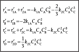
Net Rates

(5) $\begin{matrix} r_{A}^{'} = r_{1 A}^{'} + r_{2A}^{'} & (E8-5.5) \end{matrix}$ $\begin{matrix} r_{A}^{'} = r_{1 A}^{'} + r_{2A}^{'} & (E8-5.5) \end{matrix}$

(6) $\begin{matrix} r_{B}^{'} = r_{1 B}^{'} & (E8-5.6) \end{matrix}$ $\begin{matrix} r_{B}^{'} = r_{1 B}^{'} & (E8-5.6) \end{matrix}$

(7) $\begin{matrix} r_{C}^{'} = r_{1 C}^{'} + r_{2C}^{'} & (E8-5.7) \end{matrix}$ $\begin{matrix} r_{C}^{'} = r_{1 C}^{'} + r_{2C}^{'} & (E8-5.7) \end{matrix}$

(8) $\begin{matrix} r_{D}^{'} = r_{2 D}^{'} & (E8-5.8) \end{matrix}$ $\begin{matrix} r_{D}^{'} = r_{2 D}^{'} & (E8-5.8) \end{matrix}$

Rate Laws

(9) $\begin{matrix} r_{1 A}^{'} = - k_{_{1A}} C_{A} C_{B}^{2} & (E8-5.9) \end{matrix}$ $\begin{matrix} r_{1 A}^{'} = - k_{_{1A}} C_{A} C_{B}^{2} & (E8-5.9) \end{matrix}$

(10) $\begin{matrix} r_{2 C}^{'} = - k_{_{2 C}} C_{A}^{2} C_{C}^{3} & (E8-5.10) \end{matrix}$ $\begin{matrix} r_{2 C}^{'} = - k_{_{2 C}} C_{A}^{2} C_{C}^{3} & (E8-5.10) \end{matrix}$

Relative Rates

\begin{matrix} Reaction 1: & A+2B \to C & \frac{r_{1 A}^{'}}{- 1} = \frac{r_{1 B}^{'}}{- 2} = \frac{r_{1 C}^{'}}{1} \end{matrix}

$\begin{matrix} Reaction 1: & A+2B \to C & \frac{r_{1 A}^{'}}{- 1} = \frac{r_{1 B}^{'}}{- 2} = \frac{r_{1 C}^{'}}{1} \end{matrix}$

(11) $\begin{matrix} r_{1 B}^{'} = 2 r_{1 A}^{'} & (E8-5.11) \end{matrix}$ $\begin{matrix} r_{1 B}^{'} = 2 r_{1 A}^{'} & (E8-5.11) \end{matrix}$

(12) $\begin{matrix} r_{1 C}^{'} = r_{1 A}^{'} & (E8-5.12) \end{matrix}$ $\begin{matrix} r_{1 C}^{'} = r_{1 A}^{'} & (E8-5.12) \end{matrix}$

\begin{matrix} Reaction 2 : & 2 A+3C \to D & \frac{r_{2A}^{'}}{- 2} = \frac{r_{2 C}^{'}}{- 3} = \frac{r_{2 D}^{'}}{1} \end{matrix}

$\begin{matrix} Reaction 2 : & 2 A+3C \to D & \frac{r_{2A}^{'}}{- 2} = \frac{r_{2 C}^{'}}{- 3} = \frac{r_{2 D}^{'}}{1} \end{matrix}$

(13) $\begin{matrix} r_{2 A}^{'} = \frac{2}{3} r_{2 C}^{'} & (E8-5.13) \end{matrix}$ $\begin{matrix} r_{2 A}^{'} = \frac{2}{3} r_{2 C}^{'} & (E8-5.13) \end{matrix}$

(14) $\begin{matrix} r_{2 D}^{'} = - \frac{1}{3} r_{2 C}^{'} & (E8-5.14) \end{matrix}$ $\begin{matrix} r_{2 D}^{'} = - \frac{1}{3} r_{2 C}^{'} & (E8-5.14) \end{matrix}$

The net rates of reaction for species A, B, C, and D are

Selectivity

S_{C/D} = \frac{F_{C}}{F_{D}}

$S_{C/D} = \frac{F_{C}}{F_{D}}$

Tricks of the Trade

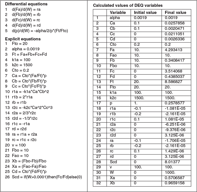
One observes that at W = 0, F_D = 0 causing S_C/D to go to infinity, Therefore, we set S_C/D = 0 between W = 0 and a very small number, W = 0.0001 kg, to prevent Polymath, as well as other ODE solvers such as MATLAB and Excel, from crashing. In Polymath, this condition is written

(15)

\begin{matrix} S_{C/D} = if (W > 0.0001) then (\frac{F_{C}}{F_{D}}) else (0) & (E8-5.15) \end{matrix}

$\begin{matrix} S_{C/D} = if (W > 0.0001) then (\frac{F_{C}}{F_{D}}) else (0) & (E8-5.15) \end{matrix}$

3. Stoichiometry Isothermal T = T₀

(16)

\begin{matrix} C_{A} = C_{T0} (\frac{F_{A}}{F_{T}}) p & (E8-5.16) \end{matrix}

$\begin{matrix} C_{A} = C_{T0} (\frac{F_{A}}{F_{T}}) p & (E8-5.16) \end{matrix}$

(17)

\begin{matrix} C_{B} = C_{T0} (\frac{F_{B}}{F_{T}}) p & (E8-5.17) \end{matrix}

$\begin{matrix} C_{B} = C_{T0} (\frac{F_{B}}{F_{T}}) p & (E8-5.17) \end{matrix}$

(18)

\begin{matrix} C_{C} = C_{T0} (\frac{F_{C}}{F_{T}}) p & (E8-5.18) \end{matrix}

$\begin{matrix} C_{C} = C_{T0} (\frac{F_{C}}{F_{T}}) p & (E8-5.18) \end{matrix}$

(19)

\begin{matrix} C_{D} = C_{T0} (\frac{F_{D}}{F_{T}}) p & (E8-5.19) \end{matrix}

$\begin{matrix} C_{D} = C_{T0} (\frac{F_{D}}{F_{T}}) p & (E8-5.19) \end{matrix}$

(20)

\begin{matrix} \frac{dp}{dW} = - \frac{α}{2 p} (\frac{F_{T}}{F_{T0}}) & (E8-5.20) \end{matrix}

$\begin{matrix} \frac{dp}{dW} = - \frac{α}{2 p} (\frac{F_{T}}{F_{T0}}) & (E8-5.20) \end{matrix}$

(21)

\begin{matrix} F_{T} = F_{A} + F_{B} + F_{C} + F_{D} & (E8-5.21) \end{matrix}

$\begin{matrix} F_{T} = F_{A} + F_{B} + F_{C} + F_{D} & (E8-5.21) \end{matrix}$

(22)

\begin{matrix} X_{A} = \frac{F_{A0} - F_{A}}{F_{A0}} & (E8-5.22A) \end{matrix}

$\begin{matrix} X_{A} = \frac{F_{A0} - F_{A}}{F_{A0}} & (E8-5.22A) \end{matrix}$

(23)

\begin{matrix} X_{B} = \frac{F_{B 0} - F_{B}}{F_{B 0}} & (E8-5.22B) \end{matrix}

$\begin{matrix} X_{B} = \frac{F_{B 0} - F_{B}}{F_{B 0}} & (E8-5.22B) \end{matrix}$

4. Parameters

(24) C_T0=0.2mol/dm³

(25) α = 0.0019 kg^-1

(26) u₀=100dm³/min

(27) k_1A = 100 (dm³/mol)²/min/kg-cat

(28) k_2C = 1,500 (dm¹⁵/mol⁴)/min/kg-cat

(29) F_T0 =20mol min

(30) F_A0 = 10

(31) F_BO = 10

Entering the above equations into Polymath’s ODE solver, we obtain the following results in Table E8-5.1 and Figures E8-5.1 and E8-5.2.

Analysis: This example is a very important one as it shows, step by step, how to handle isothermal complex reactions. For complex reactions occurring in any of the reactors shown in Figure 8-2, a numerical solution is virtually always required. The Polymath program and sample results are shown below. This problem is a Living Example Problem, LEV, so the reader can download the Polymath code and vary the reaction parameters (e.g., k_1A, α, k_2c, ν_o) to learn how Figures E8-5.1 and E8-5.2 change (http://vmriv.umich.edu/~elements/5e/08chap/live.html).

In looking at the solution we note from Figure E8-5.2 that the selectivity reaches a maximum very close to the entrance (W ≈ 60 kg) and then drops rapidly. However, 90% of A is not consumed until 200 kg, the catalyst weight at which the desired product C reaches its maximum flow rate. If the activation energy for reaction (1) is greater than that for reaction (2), try increasing the temperature to increase the molar flow rate of C and selectivity. However, if that does not help, then one has to decide which is more important, selectivity or the molar flow rate of the desired product. In the former case, the PBR catalyst weight will be 60 kg. In the latter case, the PBR catalyst weight will be 200 kg.

TABLE E8-5.1 POLYMATH PROGRAM AND OUTPUT

Graph shows four curves representing molar flow rate profiles.

Figure E8-5.1 Molar flow rate profiles.

Figure E8-5.2 Selectivity profile.

Figure shows sliders for k1a, k2c, Cto, v, alpha, and Fto. At the bottom, the Molar Flow Rates button (selected), Conversion/Pressure drop button, and Selectivity button are shown.

Figure E8-5.3 Wolfram sliders.

Graph shows Wolfram conversion profiles.

Figure E8-5.4 Wolfram conversion profiles.

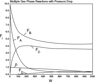
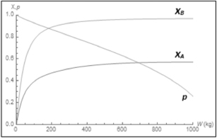
The molar flow rate profiles are shown in Figure E8-5.1, while the selectivity and conversion profiles are shown in Figures E8-5.2 and E8-5.4, respectively.

8.5.2 Complex Liquid-Phase Reactions in a CSTR

For a CSTR, a coupled set of algebraic equations analogous to the PFR differential equations must be solved. These equations are arrived at from a mole balance on CSTR for every species coupled with the rates step and stoichiometry. For q liquid-phase reactions occurring where N different species are present, we have the following set of algebraic equations:

\begin{matrix} F_{10} - F_{1} = - r_{1} V = V \sum_{i = 1}^{q} - r_{i 1} = V \cdot f_{1} (C_{1}, \dots, C_{N}) & (8 - 17) \\ ⋮ \\ F_{j 0} - F_{j} = - r_{j} V = V \cdot f_{j} (C_{1}, \dots, C_{N}) & (8 - 18) \\ ⋮ \\ F_{N 0} - F_{N} = - r_{N} V = V \cdot f_{N} (C_{1}, \dots, C_{N}) & (8 - 19) \end{matrix}

$\begin{matrix} F_{10} - F_{1} = - r_{1} V = V \sum_{i = 1}^{q} - r_{i 1} = V \cdot f_{1} (C_{1}, \dots, C_{N}) & (8 - 17) \\ ⋮ \\ F_{j 0} - F_{j} = - r_{j} V = V \cdot f_{j} (C_{1}, \dots, C_{N}) & (8 - 18) \\ ⋮ \\ F_{N 0} - F_{N} = - r_{N} V = V \cdot f_{N} (C_{1}, \dots, C_{N}) & (8 - 19) \end{matrix}$

We can use a nonlinear algebraic equation solver (NLE) in Polymath or a similar program to solve Equations (8-17) through (8-19).

..................Content has been hidden....................

You can't read the all page of ebook, please click here login for view all page.

Table of Contents for Chapter 8 Multiple Reactions

Create new playlist

Sign In

Sign Up

Multiple Reactions 8

8.1 Definitions

8.1.1 Types of Reactions

8.1.2 Selectivity

8.1.3 Yield

8.1.4 Conversion

8.2 Algorithm for Multiple Reactions

8.2.1 Modifications to the Chapter 6 CRE Algorithm for Multiple Reactions

8.3 Parallel Reactions

8.3.1 Selectivity

8.3.2 Maximizing the Desired Product for One Reactant

8.3.3 Reactor Selection and Operating Conditions

8.4 Reactions in Series

8.5 Complex Reactions

8.5.1 Complex Gas-Phase Reactions in a PBR

8.5.2 Complex Liquid-Phase Reactions in a CSTR

Table of Contents for
Chapter 8 Multiple Reactions