
10.3.7 Temperature Dependence of the Rate Law
Consider a surface-reaction-limited irreversible isomerization
in which both A and B are adsorbed on the surface, and the rate law is
The specific reaction rate, k, will usually follow an Arrhenius temperature dependence and increase exponentially with temperature. However, the adsorption of all species on the surface is exothermic. Consequently, the higher the temperature, the smaller the adsorption equilibrium constant. That is, as the temperature increases, KA and KB decrease resulting in less coverage of the surface by A and B. Therefore, at high temperatures, the denominator of catalytic rate laws approaches 1. That is, at high temperatures (low coverage)
1 ≫ (PAKA + PBKB)
The rate law could then be approximated as
Neglecting the adsorbed species at high temperatures
or for a reversible isomerization we would have
The algorithm we can use as a start in postulating a reaction mechanism and rate-limiting step is shown in Table 10-4. Again, we can never really prove a mechanism to be correct by comparing the derived rate law with experimental data. Independent spectroscopic experiments are usually needed to confirm the mechanism. We can, however, prove that a proposed mechanism is inconsistent with the experimental data by following the algorithm in Table 10-4. Rather than taking all the experimental data and then trying to build a model from the data, Box et al. describe techniques of sequential data collection and model building.14
14 G. E. P. Box, J. S. Hunter, and W. G. Hunter, Statistics for Experimenters: Design, Innovation, and Discovery, 2nd ed. (Hoboken, New Jersey: Wiley, 2005).
Algorithm
Deduce
Rate law
Find
Mechanism
Evaluate
Rate-law
parameters
Design
PBR
CSTR
10.4 Heterogeneous Data Analysis for Reactor Design
In this section we focus on four operations that chemical reaction engineers need to be able to accomplish:
(1) Developing an algebraic rate law consistent with experimental observations,
(2) Analyzing the rate law in such a manner that the rate-law parameters (e.g., k, KA) can readily be determined from the experimental data,
(3) Finding a mechanism and rate-limiting step consistent with the experimental data, and
(4) Designing a catalytic reactor to achieve a specified conversion

We shall use the hydrodemethylation of toluene to illustrate these four operations.
Hydrogen and toluene are reacted over a solid mineral catalyst containing clinoptilolite (a crystalline silica-alumina) to form methane and benzene15
15 J. Papp, D. Kallo, and G. Schay, J. Catal., 23, 168.
We wish to design a packed-bed reactor and a “fluidized bed” CSTR to process a feed consisting of 30% toluene, 45% hydrogen, and 25% inerts. Toluene is fed at a rate of 50 mol/min at a temperature of 640 C and a pressure of 40 atm (4052 kPa). To design the PBR, we must first determine the rate law from the differential reactor data presented in Table 10-6. In this table, we are given the rate of reaction of toluene as a function of the partial pressures of hydrogen (H2), toluene (T), benzene (B), and methane (M). In the first two runs, methane was introduced into the feed together with hydrogen and toluene, while the other product, benzene, was fed to the reactor together with the reactants only in runs 3, 4, and 6. In runs 5 and 16, both methane and benzene were introduced in the feed. In the remaining runs, none of the products was present in the feedstream. Because the conversion was less than 1% in the differential reactor, the partial pressures of the products, methane and benzene, formed in these runs were essentially zero, and the reaction rates were equivalent to initial rates of reaction.
10.4.1 Deducing a Rate Law from the Experimental Data
To unscramble the data let’s first look at run 3. In run 3, there is no possibility of the reverse reaction taking place because the concentration of methane is zero, i.e., PM = 0, whereas in run 5 the reverse reaction could take place because all products are present. Comparing runs 3 and 5, we see that the initial rate is essentially the same for both runs, and we can assume that the reaction is virtually irreversible.
TABLE 10-6 DATA FROM A DIFFERENTIAL REACTOR
Partial Pressure (atm) |
|||||
Run |
Toluene (T), PT |
Hydrogen P(H2), PH2 |
Methane (M), PM |
Benzene (B), PB |
|
Set A |
|||||
1 |
71.0 |
1 |
1 |
1 |
0 |
2 |
71.3 |
1 |
1 |
4 |
0 |
Set B |
|||||
3 |
41.6 |
1 |
1 |
0 |
1 |
4 |
19.7 |
1 |
1 |
0 |
4 |
5 |
42.0 |
1 |
1 |
1 |
1 |
6 |
17.1 |
1 |
1 |
0 |
5 |
Set C |
|||||
7 |
71.8 |
1 |
1 |
0 |
0 |
8 |
142.0 |
1 |
2 |
0 |
0 |
9 |
284.0 |
1 |
4 |
0 |
0 |
Set D |
|||||
10 |
47.0 |
0.5 |
1 |
0 |
0 |
11 |
71.3 |
1 |
1 |
0 |
0 |
12 |
117.0 |
5 |
1 |
0 |
0 |
13 |
127.0 |
10 |
1 |
0 |
0 |
14 |
131.0 |
15 |
1 |
0 |
0 |
15 |
133.0 |
20 |
1 |
0 |
0 |
16 |
41.8 |
1 |
1 |
1 |
1 |
Unscramble the data to find the rate law
We now ask what qualitative conclusions can be drawn from the data about the dependence of the rate of disappearance of toluene, , on the partial pressures of toluene, hydrogen, methane, and benzene.
1. Dependence on the product methane. If methane were adsorbed on the surface, the partial pressure of methane would appear in the denominator of the rate expression and the rate would vary inversely with methane concentration†
† You probably noticed that Equations (10-58) to (10-66) are missing. The reason for this is multiple choice: (a) The equations are redundant, (b) there were errors and they had to be sent to the Internet Cloud to be fixed, or (c) the author simply misnumbered the equations and is now trying to cover it up.
However, comparing runs 1 and 2 we observe that a fourfold increase in the pressure of methane has little effect on Consequently, we assume that methane is either very weakly adsorbed (i.e., or goes directly into the gas phase in a manner similar to propylene in the cumene decomposition previously discussed.


2. Dependence on the product benzene. In runs 3 and 4, we observe that, for fixed concentrations (partial pressures) of hydrogen and toluene, the rate decreases with increasing concentration of benzene. A rate expression in which the benzene partial pressure appears in the denominator could explain this dependency
The type of dependence of on PB given by Equation (10-68) suggests that benzene is adsorbed on the clinoptilolite surface.
If it is in the denominator, it is probably on the surface.
3. Dependence on toluene. At low concentrations of toluene (runs 10 and 11), the rate increases with increasing partial pressure of toluene, while at high toluene concentrations (runs 14 and 15), the rate is virtually independent of the toluene partial pressure. A form of the rate expression that would describe this behavior is
A combination of Equations (10-68) and (10-69) suggests that the rate law may be of the form

4. Dependence on hydrogen. When we compare runs 7, 8, and 9 in Table 10-6, we see that the rate increases linearly with increasing hydrogen concentration, and we conclude that the reaction is first order in H2. In light of this fact, hydrogen is either not adsorbed on the surface or its coverage of the surface is extremely low for the pressures used. If H2 were adsorbed, would have a dependence on analogous to the dependence of on the partial pressure of toluene, PT [see Equation (10-69)]. For first-order dependence on H2,
Combining Equations (10-67) through (10-71), we find that the rate law
is in qualitative agreement with the data shown in Table 10-6.
10.4.2 Finding a Mechanism Consistent with Experimental Observations
We now propose a mechanism for the hydrodemethylation of toluene. We assume that the reaction follows an Eley-Rideal mechanism where toluene is adsorbed on the surface and then reacts with hydrogen in the gas phase to produce benzene adsorbed on the surface and methane in the gas phase. Benzene is then desorbed from the surface. Because approximately 75% to 80% of all heterogeneous reaction mechanisms are surface-reaction-limited rather than adsorption- or desorption-limited, we begin by assuming the reaction between adsorbed toluene and gaseous hydrogen to be reaction-rate-limited. Symbolically, this mechanism and associated rate laws for each elementary step are
Approximately 75% of all heterogeneous reaction mechanisms are surface-reaction limited.
Proposed Mechanism
Eley–Rideal mechanism
The rate law for the surface-reaction step is
For surface-reaction-limited mechanisms we see that we need to replace CT·S and CB·S in Equation (10-73) by quantities that we can measure, e.g., concentration or partial pressure.
For surface-reaction-limited mechanisms, we use the adsorption rate Equation (10-72) for toluene to obtain CT·S16, i.e.,
16 See footnote 10 on page 444.
Then
and we use the desorption rate Equation (10-74) for benzene to obtain CB·S:
Then
The total concentration of sites is
Perform a site balance to obtain Cv.
Substituting Equations (10-75) and (10-76) into Equation (10-77) and re-arranging, we obtain
Next, substitute for CT·S and CB·S, and then substitute for Cυ in Equation (10-73) to obtain the rate law for the case when the reaction is surface-reaction-rate-limited
We have shown by comparing runs 3 and 5 that we can neglect the reverse reaction, i.e., the thermodynamic equilibrium constant KP is very, very large. Consequently, we obtain
Rate law for Eley–Rideal surface-reaction limited mechanism
Again we note that the adsorption equilibrium constant of a given species is exactly the reciprocal of the desorption equilibrium constant of that species.
10.4.3 Evaluation of the Rate-Law Parameters
In the original work on this reaction by Papp et al.,17 over 25 models were tested against experimental data, and it was concluded that the preceding mechanism and rate-limiting step (i.e., the surface reaction between adsorbed toluene and H2 gas) is the correct one. Assuming that the reaction is essentially irreversible, the rate law for the reaction on clinoptilolite is
17 Ibid.
We now wish to determine how best to analyze the data to evaluate the rate-law parameters, k, KT, and KB. This analysis is referred to as parameter estimation.18 We now rearrange our rate law to obtain a linear relationship between our measured variables. For the rate law given by Equation (10-80), we see that if both sides of Equation (10-80) are divided by PH2 PT and the equation is then inverted
18 See the Supplementary Reading for Chapter 10 (page 514) for a variety of techniques for estimating the rate-law parameters.
Linearize the rate quation to extract the rate-law parameters.
The regression techniques described in Chapter 7 could be used to determine the rate-law parameters by using the equation
One can use the linearized least-squares analysis (PRS 7.3) to obtain initial estimates of the parameters k, KT, KB, in order to obtain convergence in nonlinear regression. However, in many cases it is possible to use a nonlinear regression analysis directly, as described in Sections 7.5 and 7.6, and in Example 10-1.
A linear least-squares analysis of the data shown in Table 10-6 is presented on the CRE Web site.
Example 10-1 Nonlinear Regression Analysis to Determine the Model Parameters k, KB, and KT
(a) Use nonlinear regression, as discussed in Section 7.5, along with the data in Table 10-6, to find the best estimates of the rate-law parameters k, KB, and KT in Equation (10-80).
(b) Write the rate law solely as a function of the partial pressures.
(c) Find the ratio of the sites occupied by toluene, CT•S, to those occupied by benzene, CB•S, at 40% conversion of toluene.
Solution
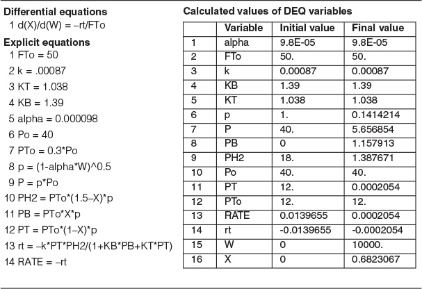
The data from Table 10-6 were entered into the Polymath nonlinear least-squares program with the following modification. The rates of reaction in column 1 were multiplied by 1010, so that each of the numbers in column 1 was entered directly (i.e., 71.0, 71.3, …). The model equation was
Following the step-by-step regression procedure in Chapter 7 and on the CRE Web site Summary Notes, we arrive at the following parameter values shown in Table E10-1.1.

Living Example Problem
(a) The best estimates are shown in the upper-right-hand box of Table E10-1.1.
(b) Converting the rate law to kilograms of catalyst and minutes,
we have
(c) After we have the adsorption constants, KT and KB, we can calculate the ratio of sites occupied by the various adsorbed species. For example, taking the ratio of Equation (10-75) to Equation (10-76), the ratio of toluene-occupied sites to benzene-occupied sites at 40% conversion is
We see that at 40% conversion there are approximately 12% more sites occupied by toluene than by benzene. This fact is common knowledge to every chemical engineering student at Jofostan University, Riça, Jofostan.
Analysis: This example shows once again how to determine the values of rate-law parameters from experimental data using Polymath regression. It also shows how to calculate the different fraction of sites, both vacant and occupied, as a function of conversion.
10.4.4 Reactor Design
Our next step is to express the partial pressures PT, PB, and PH2 as a function of X, combine the partial pressures with the rate law, , as a function of conversion, and carry out the integration of the packed-bed design equation
Example 10-2 Catalytic Reactor Design
The hydrodemethylation of toluene is to be carried out in a PBR catalytic reactor.
Living Example Problem
The molar feed rate of toluene to the reactor is 50 mol/min, and the reactor inlet is at 40 atm and 640°C. The feed consists of 30% toluene, 45% hydrogen, and 25% inerts. Hydrogen is used in excess to help prevent coking. The pressure-drop parameter, α, is 9.8 × 10⁻⁵ kg–1.
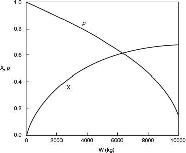
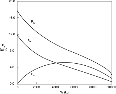
(a) Plot and analyze the conversion, the pressure ratio, p, and the partial pressures of toluene, hydrogen, and benzene as a function of PBR catalyst weight.
(b) Determine the catalyst weight in a fluidized CSTR with a bulk density of 400 kg/m3 (0.4 g/cm3) to achieve 65% conversion.
(a) PBR with pressure drop
1. Mole Balance:
Balance on toluene (T), the limiting reactant
2. Rate Law: From Equation (E10-1.1) we have
with k 0.00087 mol/atm2/kg-cat/min, KB = 1.39 atm–1, and KT = 1.038 atm–1.
3. Stoichiometry:
Relating Toluene (T) Benzene (B) Hydrogen (H2)
Because ε = 0, we can use the integrated form of the pressure-drop term.
P0 total pressure at the entrance
Note that PT0 designates the inlet partial pressure of toluene. In this example, the inlet total pressure is designated P0 to avoid any confusion. The inlet mole fraction of toluene is 0.3 (i.e., yT0 0.3), so that the inlet partial pressure of toluene is
PT0 = (0.3)(40) = 12 atm
We now calculate the maximum catalyst weight we can have, such that the exiting pressure will not fall below atmospheric pressure (i.e., 1.0 atm) for the specified feed rate. This weight is calculated by substituting the entering pressure of 40 atm and the exiting pressure of 1 atm into Equation (5-33), i.e.,
Pressure drop in PBRs is discussed in Section 5.5.
4. Evaluate: Consequently, we will set our final weight at 10,000 kg and determine the conversion profile as a function of catalyst weight up to this value. Equations (E10-2.1) through (E10-2.5) are shown in the Polymath program in Table E10-2.1. The conversion is shown as a function of catalyst weight in Figure E10-2.1, and profiles of the partial pressures of toluene, hydrogen, and benzene are shown in Figure E10-2.2. We note that the pressure drop causes (cf. Equation E10-2.5) the partial pressure of benzene to go through a maximum as one traverses the reactor.
Living Example Problem
Conversion profile down the packed bed

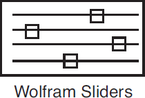
Wolfram Sliders
Note the partial pressure of benzene goes through a maximum. Why?
PBR Analysis: For the case of no pressure drop, the conversion that would have been achieved with 10,000 kg of catalyst would have been 79%, compared with 68.2% when there is pressure drop in the reactor. To carry out this calculation, for the case of no pressure drop, we use the Polymath Living Example Program (LEP) on the CRE Web site and simply multiply the pressure-drop parameter by zero, i.e., line (5) would read α = 0.00098*0. For the feed rate given, eliminating or minimizing pressure drop would increase the production of benzene by up to 61 million pounds per year! Finally, we note in Figure E10-2.2 that the partial pressure of benzene (PB) goes through a maximum. This maximum can be explained by recalling that PB is just the product of the benzene mole fraction (yB) times the total pressure (P) [i.e., PB = yBPT]. Near the middle to end of the bed, benzene is no longer being formed so that yB stops increasing. However, because of the pressure drop, the total pressure decreases and, as a result, so does PB.
If one had neglected ΔP it could have been very embarrassing.
See YouTube video, “Reaction Engineering Gone Wrong,” accessible from the CRE Web site home page.
(b) Fluidized CSTR
We will now calculate the fluidized CSTR catalyst weight necessary to achieve the same (ca.) conversion as in the packed-bed reactor at the same operating conditions. The bulk density in the fluidized reactor is 0.4 g/cm3. The design equation is
1. Mole Balance:
Rearranging

2. Rate Law and 3. Stoichiometry same as in part (a) PBR calculation
4. Combine and Evaluate: Writing Equation (E10-2.2) in terms of conversion (E10-2.3) and then substituting X = 0.65 and PT0 = 12 atm, we have
The corresponding reactor volume is
This volume would correspond to a cylindrical reactor 2 meters in diameter and 10 meters high.
Analysis: This example used real data and the CRE algorithm to design a PBR and CSTR. An important point is that it showed how one could be embarrassed by not including pressure drop in the design of a packed-bed reactor. We also note that for both the PBR and fluidized CSTR, the values of the catalyst weight and reactor volume are quite high, especially for the low feed rates given. Consequently, the temperature of the reacting mixture should be increased to reduce the catalyst weight, provided that side reactions and catalyst decay do not become a problem at higher temperatures.
How can the weight of catalyst be reduced? Raise the temperature?
Example 10-2 illustrated the major activities pertinent to catalytic reactor design described earlier in Figure 10-6. In this example, the rate law was extracted directly from the data and then a mechanism was found that was consistent with experimental observation. Conversely, developing a feasible mechanism may guide one in the synthesis of the rate law.
10.5 Reaction Engineering in Microelectronic Fabrication
10.5.1 Overview
We now extend the principles of the preceding sections to one of the newer technologies in chemical engineering. Chemical engineers are now playing an important role in the electronics industry. Specifically, they are becoming more involved in the manufacture of electronic and photonic devices, recording materials, and especially medical lab-on-a-chip devices.
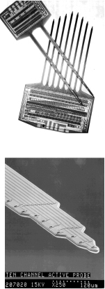
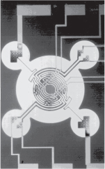
Surface reactions play an important role in the manufacture of microelectronic devices. One of the single most important developments of the twentieth century was the invention of the integrated circuit. Advances in the development of integrated circuitry have led to the production of circuits that can be placed on a single semiconductor chip the size of a pinhead and perform a wide variety of tasks by controlling the electron flow through a vast network of channels. These channels, which are made from semiconductors such as silicon, gallium arsenide, indium phosphide, and germanium, have led to the development of a multitude of novel microelectronic devices. Examples of microelectronic sensing devices manufactured using chemical reaction engineering principles are shown in the left-hand margin.
The manufacture of an integrated circuit requires the fabrication of a network of pathways for electrons. The principal reaction engineering steps of the fabrication process include depositing material on the surface of a material called a substrate (e.g., by chemical vapor deposition, abbreviated as CVD), changing the conductivity of regions of the surface (e.g., by boron doping or ion inplantation), and removing unwanted material (e.g., by etching). By applying these steps systematically, miniature electronic circuits can be fabricated on very small semiconductor chips. The fabrication of microelectronic devices may include as few as 30 or as many as 200 individual steps to produce chips with up to 109 elements per chip.
An abbreviated schematic of the steps involved in producing a typical metal-oxide, semiconductor, field-effect transistor (MOSFET) device is shown in Figure 10-20. Starting from the upper left, we see that single-crystal silicon ingots are grown in a Czochralski crystallizer, sliced into wafers, and chemically and physically polished. These polished wafers serve as starting materials for a variety of microelectronic devices. A typical fabrication sequence is shown for processing the wafer, beginning with the formation of an SiO2 layer on top of the silicon. The SiO2 layer may be formed either by oxidizing a silicon layer or by laying down a layer of SiO2 by chemical vapor deposition (CVD). Next, the wafer is masked with a polymer photoresist, a template with the pattern to be etched onto the SiO2 layer is placed over the photoresist, and the wafer is exposed to ultraviolet irradiation. If the mask is a positive photoresist, the light will cause the exposed areas of the polymer to dissolve when the wafer is placed in the developer. On the other hand, when a negative photoresist mask is exposed to ultraviolet irradiation, cross-linking of the polymer chains occurs, and the unexposed areas dissolve in the developer. The undeveloped portion of the photoresist (in either case) will protect the covered areas from etching.
Chemical engineering principles are involved in virtually every step!
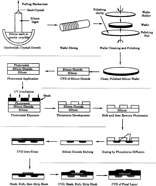
After the exposed areas of SiO2 are etched to form trenches (either by wet etching or by plasma etching), the remaining photoresist is removed. Next, the wafer is placed in a furnace containing gas molecules of the desired dopant, which then diffuse into the exposed silicon. After diffusion of dopant to the desired depth in the wafer, the wafer is removed and then SiO2 is removed by etching. The sequence of masking, etching, CVD, and metallization continues until the desired device is formed. A schematic of a final chip is shown in the lower-right-hand corner of Figure 10-20. In Section 10.5.2, we discuss one of the key processing steps, CVD.
10.5.2 Chemical Vapor Deposition
The mechanisms by which CVD occurs are very similar to those of heterogeneous catalysis discussed earlier in this chapter. The reactant(s) adsorbs on the surface and then reacts on the surface to form a new surface. This process may be followed by a desorption step, depending on the particular reaction.
Ge used in solar cells
The growth of a germanium epitaxial film as an interlayer between a gallium arsenide layer and a silicon layer has received attention in the microelectronics industry.19 Epitaxial germanium is also an important material in the fabrication of tandem solar cells. The growth of germanium films can be accomplished by CVD. A proposed mechanism is
Mechanism
19 H. Ishii and Y. Takahashi, J. Electrochem. Soc., 135, p. 1539.
At first it may appear that a site has been lost when comparing the right- and left-hand sides of the surface reaction step. However, the newly formed germanium atom on the right-hand side is a site for the future adsorption of H2(g) or GeCl2(g), and there are three sites on both the right- and left-hand sides of the surface reaction step. These sites are shown schematically in Figure 10-21.
The surface reaction between adsorbed molecular hydrogen and germanium dichloride is believed to be rate-limiting. The reaction follows an elementary rate law with the rate being proportional to the fraction of the surface covered by GeCl2 times the square of the fraction of the surface covered by molecular hydrogen.

where
The deposition rate (film growth rate) is usually expressed in nanometers per second and is easily converted to a molar rate (mol/m2 s) by multiplying by the molar density of solid germanium (mol/m3).
The difference between developing CVD rate laws and rate laws for catalysis is that the site concentration (e.g., Cυ ) is replaced by the fractional surface area coverage (e.g., the fraction of the surface that is vacant, fv). The total fraction of surface available for adsorption should, of course, add up to 1.0.
Area balance
We will first focus our attention on the adsorption of GeCl2. The rate of jumping on to the surface is proportional to the partial pressure of GeCl2, PGeCl2, and the fraction of the surface that is vacant, fv. The net rate of GeCl2 adsorption is
Since the surface reaction is rate-limiting, in a manner analogous to catalysis reactions, we have for the adsorption of GeCl2
Adsorption of GeCl2 not rate-limiting
Solving Equation (10-84) for the fractional surface coverage of GeCl2 gives
For the dissociative adsorption of hydrogen on the Ge surface, the equation analogous to Equation (10-84) is
Since the surface reaction is rate-limiting Then
Adsorption of H2 is not rate-limiting
Then
Recalling the rate of deposition of germanium, we substitute for and fH in Equation (10-82) to obtain
We solve for fv in an identical manner to that for Cv in heterogeneous catalysis. Substituting Equations (10-85) and (10-87) into Equation (10-83) gives
Rearranging yields
Finally, substituting for fv in Equation (10-88), we find that
and lumping KA, KH, and kS into a specific reaction rate k′ yields
Rate of deposition of Ge
We now need to relate the partial pressure of GeCl2 to the partial pressure of GeCl4 in order to calculate the conversion of GeCl4. If we assume that the gas-phase reaction
Equilibrium in gas phase
is in equilibrium, we have
and if hydrogen is weakly adsorbed , we obtain the rate of deposition as
We now can use stoichiometry to express each of the species’ partial pressures in terms of conversion and the entering partial pressure of GeCl4, , and then proceed to calculate the conversion.
It should also be noted that it is possible that GeCl2 may also be formed by the reaction of GeCl4 and a Ge atom on the surface, in which case a different rate law would result.
Rate of deposition of Ge when H2 is weakly adsorbed
10.6 Model Discrimination
We have seen that for each mechanism and each rate-limiting step we can derive a rate law. Consequently, if we had three possible mechanisms and three rate-limiting steps for each mechanism, we would have nine possible rate laws to compare with the experimental data. We will use the regression techniques discussed in Chapter 7 to identify which model equation best fits the data by choosing the one with the smaller sums of squares and/or carrying out an F-test. We could also compare the nonlinear regression residual plots for each model, which not only show the error associated with each data point but also show if the error is randomly distributed or if there is a trend in the error. If the error is randomly distributed, this result is an additional indication that the correct rate law has been chosen.

Regression
We need to raise a caution here about choosing the model with the smallest sums of squares. The caution is that the model parameter values that give the smallest sum must be realistic. In the case of heterogeneous catalysis, all values of the adsorption equilibrium constants must be positive. In addition, if the temperature dependence is given, because adsorption is exothermic, the adsorption equilibrium constant must decrease with increasing temperature. To illustrate these principles, let’s look at the following example.

Example 10-3 Hydrogenation of Ethylene to Ethane
The hydrogenation (H) of ethylene (E) to form ethane (EA),
is carried out over a cobalt molybdenum catalyst [Collect. Czech. Chem. Commun., 51, 2760 (1988)]. Carry out a nonlinear regression analysis to determine which of the following rate laws best describes the data in Table E10-3.1.
(a)
(b)
(c)
(d)
TABLE E10-3.1 DIFFERENTIAL REACTOR DATA
| Run Number | Reaction Rate (mol/kg-cat.s) | PE (atm) | PEA (atm) | PH (atm) |
1 |
1.04 |
1 |
1 |
1 |
2 |
3.13 |
1 |
1 |
3 |
3 |
5.21 |
1 |
1 |
5 |
4 |
3.82 |
3 |
1 |
3 |
5 |
4.19 |
5 |
1 |
3 |
6 |
2.391 |
0.5 |
1 |
3 |
7 |
3.867 |
0.5 |
0.5 |
5 |
8 |
2.199 |
0.5 |
3 |
3 |
9 |
0.75 |
0.5 |
5 |
1 |
Procedure
• Enter data
• Enter model
• Make initial estimates of parameters
• Run regression
• Examine parameters and variance
• Observe error distribution
• Choose model
Solution
Polymath was chosen as the software package to solve this problem. The data in Table E10-3.1 were entered into the program. A screen-shot-by-screen-shot set of instructions on how to carry out the regression is given on the CRE Web site, at the end of the Summary Notes for Chapter 7 (http://www.umich.edu/~elements/5e/07chap/summary.html). After entering the data and following the step-by-step procedures, the results shown in Table E10-3.2 were obtained.


TABLE E10-3.2 RESULTS OF THE POLYMATH NONLINEAR REGRESSION

Model (a) Single site, surface-reaction, rate-limited with hydrogen weakly adsorbed
From Table E10-3.2 we can obtain
We now examine the sums of squares (variance) and range of variables themselves. The sums of squares is reasonable and, in fact, the smallest of all the models at 0.0049. However, let’s look at KEA. We note that the value for the 95% confidence limit of ±0.0636 is greater than the nominal value of KEA = 0.043 atm–1 itself (i.e., KEA = 0.043 ± 0.0636). The 95% confidence limit means that if the experiment were run 100 times and then 95 times it would fall within the range (–0.021) < KEA < (0.1066). Because KEA can never be negative, we are going to reject this model. Consequently, we set KEA = 0 and proceed to Model (b).
Model (b) Single site, surface-reaction, rate-limited with ethane and hydrogen weakly adsorbed
From Table E10-3.2 we can obtain
The value of the adsorption constant KE = 2.1 atm–1 is reasonable and is not negative within the 95% confidence limit. Also, the variance is small at = 0.0061.
Model (c) Dual site, surface-reaction, rate-limited with hydrogen and ethane weakly adsorbed
From Table E10-3.2 we can obtain
While KE is small, it never goes negative within the 95% confidence interval. The variance of this model at is much larger than the other models. Comparing the variance of model (c) with model (b)
We see that the is an order of magnitude greater than , and therefore we eliminate model (c).20
20 See G. F. Froment and K. B. Bishoff, Chemical Reaction Analysis and Design, 2nd ed. (New York: Wiley, 1990), p. 96.
Model (d) Empirical
Similarly for the power law model, we obtain from Table E10-3.2
As with model (c), the variance is quite large compared to model (b)
So we also eliminate model (d). For heterogeneous reactions, Langmuir-Hinshel-wood rate laws are preferred over power-law models.
Analysis: Choose the Best Model. In this example, we were presented with four rate laws and were asked which law best fits the data. Because all the parameter values are realistic for model (b) and the sums of squares are significantly smaller for model (b) than for the other models, we choose model (b). We note again that there is a caution we need to point out regarding the use of regression! One cannot simply carry out a regression and then choose the model with the lowest value of the sums of squares. If this were the case, we would have chosen model (a), which had the smallest sums of squares of all the models with σ2 = 0.0049. However, one must consider the physical realism of the parameters in the model. In model (a) the 95% confidence interval was greater than the parameter itself, thereby yielding negative values of the parameter, KAE, which is physically impossible.
10.7 Catalyst Deactivation
In designing fixed and ideal fluidized-bed catalytic reactors, we have assumed up to now that the activity of the catalyst remains constant throughout the catalyst’s life. That is, the total concentration of active sites, Ct, accessible to the reaction does not change with time. Unfortunately, Mother Nature is not so kind as to allow this behavior to be the case in most industrially significant catalytic reactions. One of the most insidious problems in catalysis is the loss of catalytic activity that occurs as the reaction takes place on the catalyst. A wide variety of mechanisms have been proposed by Butt and Petersen, to explain and model catalyst deactivation.21, 22, 23
21 J. B. Butt and E. E. Petersen, Activation, Deactivation and Poisoning of Catalysts (New York: Academic Press, 1988).
22 D. T. Lynch and G. Emig, Chem. Eng. Sci., 44(6), 1275–1280 (1989).
23 R. Hughes, Deactivation of Catalysts (San Diego: Academic Press, 1984).
Catalytic deactivation adds another level of complexity to sorting out the reaction rate law parameters and pathways. In addition, we need to make adjustments for the decay of the catalysts in the design of catalytic reactors. However, please don’t worry, this adjustment is usually made by a quantitative specification of the catalyst’s activity, a(t). In analyzing reactions over decaying catalysts, we divide the reactions into two categories: separable kinetics and non-separable kinetics. In separable kinetics, we separate the rate law and activity
Separable kinetics: = a (Past history) × (Fresh catalyst)
When the kinetics and activity are separable, it is possible to study catalyst decay and reaction kinetics independently. However, nonseparability
Nonseparable kinetics: = (Past history, fresh catalyst)
must be accounted for by assuming the existence of a nonideal surface or by describing deactivation by a mechanism composed of several elementary steps.22
We shall consider only separable kinetics and define the activity of the catalyst at time t, a(t), as the ratio of the rate of reaction on a catalyst that has been used for a time t to the rate of reaction on a fresh catalyst (t = 0):
Because of the catalyst decay, the activity decreases with time and a typical curve of the activity as a function of time is shown in Figure 10-22.

Combining Equations (10-92) and (3-2), the rate of disappearance of reactant A on a catalyst that has been utilized for a time t is
where a(t) |
= catalytic activity, time-dependent |
k(T) |
= specific reaction rate, temperature-dependent |
Ci |
= gas-phase concentration of reactants, products, or contaminant |
Reaction rate law accounting for catalyst activity
The rate of catalyst decay, rd, can be expressed in a rate law analogous to Equation (10-93)
Catalyst decay rate law
e.g., p[a(t)] = [a(t)]2
where p[a(t)] is some function of the catalyst activity, kd is the specific decay constant, and h(Ci) is the functionality of rate of decay, rd, on the species concentrations in the reacting mixture. For the cases presented in this chapter, this functionality either will be independent of concentration (i.e., h = 1) or will be a linear function of species concentration (i.e., h = Ci).
The functionality of the activity term, p[a(t)], in the decay law can take a variety of forms. For example, for a first-order decay
and for a second-order decay
The particular function, p(a), will vary with the gas catalytic system being used and the reason or mechanism for catalytic decay.
10.7.1 Types of Catalyst Deactivation
There are three categories into which the loss of catalytic activity can traditionally be divided: sintering or aging, fouling or coking, and poisoning.
• Sintering
• Fouling
• Poisoning
Deactivation by Sintering (Aging).24 Sintering, also referred to as aging, is the loss of catalytic activity due to a loss of active surface area resulting from the prolonged exposure to high gas-phase temperatures. The active surface area may be lost either by crystal agglomeration and growth of the metals deposited on the support or by narrowing or closing of the pores inside the catalyst pellet. A change in the surface structure may also result from either surface recrystallization or the formation or elimination of surface defects (active sites). The reforming of heptane over platinum on alumina is an example of catalyst deactivation as a result of sintering.
24 See G. C. Kuczynski, ed., Sintering and Catalysis, vol. 10 of Materials Science Research (New York: Plenum Press, 1975).
Figure 10-23 shows the loss of surface area resulting from the flow of the solid porous catalyst support at high temperatures to cause pore closure. Figure 10-24 shows the loss of surface area by atomic migration and agglomeration of small metal sites deposited on the surface into a larger site where the interior atoms are not accessible to the reaction. Sintering is usually negligible at temperatures below 40% of the melting temperature of the solid.25
The catalyst support becomes soft and flows, resulting in pore closure.
25 R. Hughes, Deactivation of Catalysts (San Diego: Academic Press, 1984).
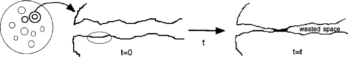

Figure 10-24 Decay by sintering: agglomeration of deposited metal sites; loss of reactive surface area.
The atoms move along the surface and agglomerate.
Deactivation by sintering may in some cases be a function of the mainstream gas concentration. Although other forms of the sintering decay rate laws exist, one of the most commonly used decay laws is second order with respect to the present activity
Integrating, with a = 1 at time t = 0, yields
Sintering: second-order decay
The amount of sintering is usually measured in terms of the active surface area of the catalyst Sa
The sintering decay constant, kd, follows the Arrhenius equation
The decay activation energy, Ed, for the reforming of heptane on Pt/Al2O3 is on the order of 70 kcal/mol, which is rather high. As mentioned earlier, sintering can be reduced by keeping the temperature below 0.3 to 0.4 times the metal’s melting point temperature, i.e., (T < 0.3 Tmelting).
Minimizing sintering
We will now stop and consider reactor design for a fluid–solid system with decaying catalyst. To analyze these reactors, we only add one step to our algorithm; that is, determine the catalyst decay law. The sequence is shown here.
The algorithm
Example 10-4 Calculating Conversion with Catalyst Decay in Batch Reactors
The first-order isomerization
A → B
is being carried out isothermally in a batch reactor on a catalyst that is decaying as a result of aging. Derive an equation for conversion as a function of time.
Solution
1. Mol Balance:
where Xd is the conversion of A when the catalyst is decaying.
2. Reaction-Rate Law:
3. Decay Law: For second-order decay by sintering:
One extra step (number 3) is added to the algorithm.
5. Combining gives us
Let k = k’W/V. Substituting for catalyst activity a, we have
where Xd is the conversion when there is decay. We want to compare the conversion with and without catalyst decay.
For no decay kd = 0
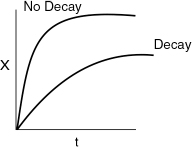
The Polymath program and a comparison of the conversion with decay Xd and without decay X are shown below.

Analytical Solution
One can also obtain an analytical solution for this reaction order and low decay. Separating variables and integrating yields
6. Solving for the conversion Xd at any time, t, in a decaying catalyst we find that
the analytical solution without decay
Parameters
E = 20,000cal/mol
k1 = 0.01S−1
T1 = 300K
k1d = 0.1
T2 = 300
Ed = 75,000cal/mol
R = 1.987
Analysis: One observes that for long times the conversion in reactors with catalyst decay approaches a rather flat plateau and reaches conversion of about 30%. This is the conversion that will be achieved in a batch reactor for a first-order reaction when the catalyst decay law is second order. By comparison, we obtain virtually complete conversion in 500 minutes when there is no decay. The purpose of this example was to demonstrate the algorithm for isothermal catalytic reactor design for a decaying catalyst. In problem P10-1B(d) you are asked to sketch the temperature–time trajectories for various values of k and kd.
Deactivation by Coking or Fouling This mechanism of decay (see Figures 10-25 and 10-26) is common to reactions involving hydrocarbons. It results from a carbonaceous (coke) material being deposited on the surface of a catalyst. The amount of coke on the surface after a time t has been found to obey the following empirical relationship
where CC is the concentration of carbon on the surface (g/m2) and n and A are empirical fouling parameters, which can be functions of the feed rate. This expression was originally developed by Voorhies and has been found to hold for a wide variety of catalysts and feed streams.26 Representative values of A and n for the cracking of East Texas light gas oil yield27
26 A. Voorhies, Ind. Eng. Chem., 37, 318 (1945).
27 C. O. Prater and R. M. Lago, Adv. Catal., 8, 293 (1956).
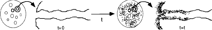
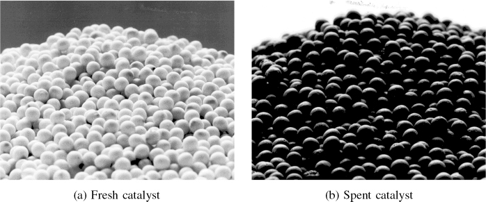
Figure 10-26 Decay by coking. (Photos courtesy of Engelhard catalyst, copyright by Michael Gaffney Photographer, Mendham, NJ.)
Different functionalities between the activity and amount of coke on the surface have been observed. One commonly used form is
or, in terms of time, we combine Equations (10-101) and (10-102)
For light Texas gas oil being cracked at 750°F over a synthetic catalyst for short times, the decay law is
where t is in seconds.
Other commonly used forms are
Activity for deactivation by coking
and
A dimensionless fouling correlation has been developed by Pacheco and Petersen.28
28 M. A. Pacheco and E. E. Petersen, J. Catal., 86, 75 (1984).
When possible, coking can be reduced by running at elevated pressures (2000 to 3000 kPa) and hydrogen-rich streams. A number of other techniques for minimizing fouling are discussed by Bartholomew.29 Catalysts deactivated by coking can usually be regenerated by burning off the carbon.
29 R. J. Farrauto and C. H. Bartholomew, Fundamentals of Industrial Catalytic Processes, 2nd edition (New York: Blackie Academic and Professional, 2006). This book is one of the most definitive resources on catalyst decay.
Minimizing coking
Deactivation by Poisoning. Deactivation by this mechanism occurs when the poisoning molecules become irreversibly chemisorbed to active sites, thereby reducing the number of sites available for the main reaction. The poisoning molecule, P, may be a reactant and/or a product in the main reaction, or it may be an impurity in the feed stream.
It’s going to cost you.
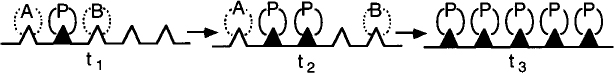
Poison in the Feed. Many petroleum feed stocks contain trace impurities such as sulfur, lead, and other components that are too costly to remove, yet poison the catalyst slowly over time. For the case of an impurity, P, in the feed stream, such as sulfur, for example, in the reaction sequence
the surface sites would change with time as shown in Figure 10-27.
Progression of sites being poisoned
If we assume the rate of removal of the poison, rP⋅S, from the reactant gas stream onto the catalyst sites is proportional to the number of sites that are unpoisoned (Ct0 – CP . S) and the concentration of poison in the gas phase is CP then
where CP˙S is the concentration of poisoned sites and Ct0 is the total number of sites initially available. Because every molecule that is adsorbed from the gas phase onto a site is assumed to poison the site, this rate is also equal to the rate of removal of total active sites (Ct) from the surface
Dividing through by Ct0 and letting f be the fraction of the total number of sites that have been poisoned yields
The fraction of sites available for adsorption (1 − f) is essentially the activity a(t). Consequently, Equation (10-108) becomes
A number of examples of catalysts with their corresponding catalyst poisons are given by Farrauto and Bartholomew.30
30 Ibid.
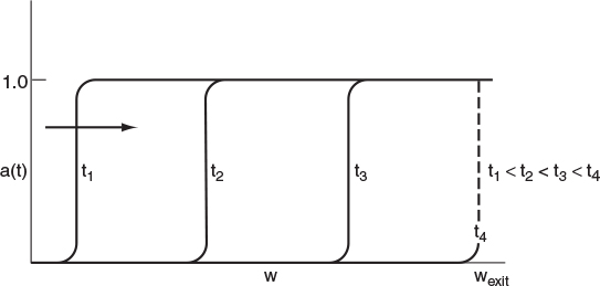
Packed-Bed Reactors. In packed-bed reactors where the poison is removed from the gas phase by being adsorbed on the specific catalytic sites, the deactivation process can move through the packed bed as a wave front. Here, at the start of the operation, only those sites near the entrance to the reactor will be deactivated because the poison (which is usually present in trace amounts) is removed from the gas phase by the adsorption; consequently, the catalyst sites farther down the reactor will not be affected. However, as time continues, the sites near the entrance of the reactor become saturated, and the poison must travel farther downstream before being adsorbed (removed) from the gas phase and attaching to a site to deactivate it. Figure 10-28 shows the corresponding activity profile for this type of poisoning process. We see in Figure 10-28 that by time t4 the entire bed has become deactivated. The corresponding overall conversion at the exit of the reactor might vary with time as shown in Figure 10-29. The partial differential equations that describe the movement of the reaction front shown in Figure 10-28 are derived and solved in an example on the CRE Web site, at the very end of the Summary Notes for Chapter 10 (http://www.umich.edu/~elements/5e/10chap/summary.html).


Poisoning by Either Reactants or Products. For the case where the main reactant also acts as a poison, the rate laws are
An example where one of the reactants acts as a poison is in the reaction of CO and H2 over ruthenium to form methane, with
Similar rate laws can be written for the case when the product B acts as a poison.
For separable deactivation kinetics resulting from contacting a poison at a constant concentration and no spatial variation
Separable deactivation kinetics
where . The solution to this equation for the case of first-order decay, n = 1
is
Empirical Decay Laws. Table 10-7 gives a number of empirical decay laws along with the reaction systems to which they apply.
One should also see Fundamentals of Industrial Catalytic Processes, by Farrauto and Bartholomew, which contains rate laws similar to those in Table 10-7, and also gives a comprehensive treatment of catalyst deactivation.31
31 Ibid.
Key resource for catalyst deactivation
Functional Form of Activity |
Decay Reaction Order |
Differential Form |
Integral Form |
Examples |
Linear |
0 |
Conversion of para-hydrogen on tungsten when poisoned with oxygena |
||
Exponential |
1 |
Ethylene hydrogenation on Cu poisoned with COb |
||
|
|
|
|
Paraffin dehydrogenation on Cr? Al2O3c |
Hyperbolic |
2 |
Vinyl chloride monomer formationf |
||
Reciprocal power |
Cracking of gas oil and gasoline on clayi |
|||
|
Cyclohexane aromatization on NiAlj |
a D. D. Eley and E. J. Rideal, Proc. R. Soc. London, A178, 429 (1941).
b R. N. Pease and L. Y. Steward, J. Am. Chem. Soc., 47, 1235 (1925).
c E. F. K. Herington and E. J. Rideal, Proc. R. Soc. London, A184, 434 (1945).
d V. W. Weekman, Ind. Eng. Chem. Process Des. Dev., 7, 90 (1968).
e A. F. Ogunye and W. H. Ray, Ind. Eng. Chem. Process Des. Dev., 9, 619 (1970).
f A. F. Ogunye and W. H. Ray, Ind. Eng. Chem. Process Des. Dev., 10, 410 (1971).
g H. V. Maat and L. Moscou, Proc. 3rd lnt. Congr. Catal. (Amsterdam: North-Holland, 1965), p. 1277.
h A. L. Pozzi and H. F. Rase, Ind. Eng. Chem., 50, 1075 (1958).
i A. Voorhies, Jr., Ind. Eng. Chem., 37, 318 (1945); E. B. Maxted, Adv. Catal., 3, 129 (1951).
j C. G. Ruderhausen and C. C. Watson, Chem. Eng. Sci., 3, 110 (1954).
Source: J. B. Butt, Chemical Reactor Engineering–Washington, Advances in Chemistry Series 109 (Washington, D.C.: American Chemical Society, 1972), p. 259. Also see CES 23, 881(1968).
Examples of reactions with decaying catalysts and their decay laws
10.8 Reactors That Can Be Used to Help Offset Catalyst Decay
We will now consider three reaction systems that can be used to handle systems with decaying catalyst. We will classify these systems as those having slow, moderate, and rapid losses of catalytic activity. To offset the decline in chemical reactivity of decaying catalysts in continuous-flow reactors, the following three methods are commonly used:
Matching the reactor type with speed of catalyst decay
• Slow decay – Temperature–Time Trajectories (10.8.1)
• Moderate decay – Moving-Bed Reactors (10.8.2)
• Rapid decay – Straight-Through Transport Reactors (10.8.3)
10.8.1 Temperature–Time Trajectories
In many large-scale reactors, such as those used for hydrotreating, and reaction systems where deactivation by poisoning occurs, the catalyst decay is relatively slow. In these continuous flow systems, constant conversion is usually necessary in order that subsequent processing steps (e.g., separation) are not upset. One way to maintain a constant conversion with a decaying catalyst in a packed or fluidized bed is to increase the reaction rate by steadily increasing the feed temperature to the reactor. Operation of a “fluidized” bed in this manner is shown in Figure 10-30.

We are going to increase the feed temperature, T, in such a manner that the reaction rate remains constant with time:
For a first-order reaction we have
Slow rate of catalyst decay
We will neglect any variations in concentration so that the product of the activity (a) and specific reaction rate (k) is constant and equal to the specific reaction rate, k0 at time t = 0 and temperature T0; that is
Gradually raising the temperature can help offset effects of catalyst decay.
The goal is to find how the temperature should be increased with time (i.e., the temperature–time trajectory) to maintain constant conversion. Using the Arrhenius equation to substitute for k in terms of the activation energy, EA, gives
Solving for 1/T yields
The decay law also follows an Arrhenius-type temperature dependence
where kd0 |
= decay constant at temperature T0, s-1 |
EA |
= activation energy for the main reaction (e.g., A → B), kJ/mol |
Ed |
= activation energy for catalyst decay, kJ/mol |
Substituting Equation (10-115) into (10-116) and rearranging yields
Integrating with a = 1 at t = 0 for the case n ≠ (1 + Ed/EA), we obtain
Solving Equation (10-114) for a and substituting in (10-118) gives
Equation (10-119) tells us how the temperature of the catalytic reactor should be increased with time in order for the reaction rate to remain constant. However one would first want to solve this equation for temperature, T, as a function of time, t, in order to correctly operate the preheater shown in Figure 10-30.
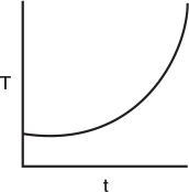
In many industrial reactions, the decay rate law changes as temperature increases. In hydrocracking, the temperature–time trajectories are divided into three regimes. Initially, there is fouling of the acidic sites of the catalyst followed by a linear regime due to slow coking and, finally, accelerated coking characterized by an exponential increase in temperature. The temperature–time trajectory for a deactivating hydrocracking catalyst is shown in Figure 10-31.
For a first-order decay, Krishnaswamy and Kittrell’s expression, Equation (10-119), for the temperature–time trajectory reduces to
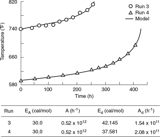
Figure 10-31 Temperature–time trajectories for deactivating hydrocracking catalyst, runs 3 and 4. (Krishnaswamy, S., and J. R. Kittrell. Analysis of Temperature–Time Data for Deactivating Catalysts. Industry and Engineering Chemistry Process Design and Development, 1979, 18(3), 399–403. Copyright © 1979, American Chemical Society. Reprinted by permission.)
Comparing theory and experiment