12. Generative Adversarial Networks
Back in Chapter 3, we introduced the idea of deep learning models that can create novel and unique pieces of visual imagery—images that we might even be able to call art. In this chapter, we combine the high-level theory from Chapter 3 with the convolutional networks from Chapter 10, the Keras Model class from Chapter 11, and a couple of new layer types, enabling you to code up a generative adversarial network (GAN) that outputs images in the style of sketches hand drawn by humans.
Essential GAN Theory
At its highest level, a GAN involves two deep learning networks pitted against each other in an adversarial relationship. As depicted by the trilobites in Figure 3.4, one network is a generator that produces forgeries of images, and the other is a discriminator that attempts to distinguish the generator’s fakes from the real thing. Moving from trilobites to slightly more-technical schematic sketches, the generator is tasked with receiving a random noise input and turning this into a fake image, as shown on the left in Figure 12.1. The discriminator—a binary classifier of real versus fake images—is shown in Figure 12.1 on the right. (The schematics in this figure are highly simplified for illustrative purposes, but we’ll go into more detail shortly.) Over several rounds of training, the generator becomes better at producing more-convincing forgeries, and so too the discriminator improves its capacity for detecting the fakes. As training continues, the two models battle it out, trying to outdo one another, and, in so doing, both models become more and more specialized at their respective tasks. Eventually this adversarial interplay can culminate in the generator producing fakes that are convincing not only to the discriminator network but also to the human eye.

Figure 12.1 Highly simplified schematic diagrams of the two models that make up a typical GAN: the generator (left) and the discriminator (right)
Training a GAN consists of two opposing (adversarial!) processes:
Discriminator training: As mapped out in Figure 12.2, in this process the generator produces fake images—that is, it performs inference only1—while the discriminator learns to tell the fake images from real ones.
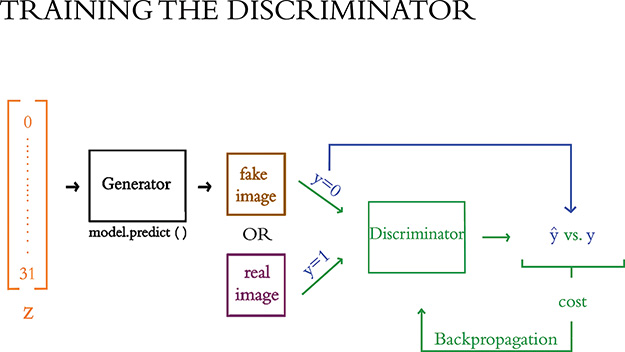
Figure 12.2 This is an outline of the discriminator training loop. Forward propagation through the generator produces fake images. These are mixed into batches with real images from the dataset and, together with their labels, are used to train the discriminator. Learning paths are shown in green, while non-learning paths are shown in black and the blue arrow calls attention to the image labels, y.
Generator training: As depicted in Figure 12.3, in this process the discriminator judges fake images produced by the generator. Here, it is the discriminator that performs inference only, whereas it’s the generator that uses this information to learn—in this case, to learn how to better fool the discriminator into classifying fake images as real ones.

Figure 12.3 An outline of the generator training loop. Forward propagation through the generator produces fake images, and inference with the discriminator scores these images. The generator is improved through backpropagation. As in Figure 12.2, learning paths are shown in green, and non-learning paths are shown in black. The blue arrow calls attention to the relationship between the image and its label y which, in the case of generator training, is always equal to 1.
1. Inference is forward propagation alone. It does not involve model training (via, e.g., backpropagation).
Thus, in each of these two processes, one of the models creates its output (either a fake image or a prediction of whether the image is fake) but is not trained, and the other model uses that output to learn to perform its task better.
During the overall process of training a GAN, discriminator training alternates with generator training. Let’s dive into both training processes in a bit more detail, starting with discriminator training (see Figure 12.2):
The generator produces fake images (by inference; shown in black) that are mixed in with batches of real images and fed into the discriminator for training.
The discriminator outputs a prediction (ŷ) that corresponds to the likelihood that the image is real.
The cross-entropy cost is evaluated for the discriminator’s ŷ predictions relative to the true y labels.
Via backpropagation tuning the discriminator’s parameters (shown in green), the cost is minimized in order to train the model to better distinguish real images from fake ones.
Note well that during discriminator training, it is only the discriminator network that is learning; the generator network is not involved in the backpropagation, so it doesn’t learn anything.
Now let’s turn our focus to the process that discriminator training alternates with: the training of the generator (shown in Figure 12.3):
The generator receives a random noise vector z as input2 and produces a fake image as an output.
The fake images produced by the generator are fed directly into the discriminator as inputs. Crucially to this process, we lie to the discriminator and label all of these fake images as real (y = 1).
The discriminator (by inference; shown in black) outputs ŷ predictions as to whether a given input image is real or fake.
Cross-entropy cost here is used to tune the parameters of the generator network (shown in green). More specifically, the generator learns how convincing its fake images are to the discriminator network. By minimizing this cost, the generator will learn to produce forgeries that the discriminator mistakenly labels as real—forgeries that may even appear to be real to the human eye.
2. This random noise vector z corresponds to the latent-space vector introduced in Chapter 3 (see Figure 3.4), and it is unrelated to the z variable that has been used since Figure 6.8 to represent w · x + b. We cover this in more detail later on in this chapter.
So, during generator training, it is only the generator network that is learning. Later in this chapter, we show you how to freeze the discriminator’s parameters so that backpropagation can tune the generator’s parameters without influencing the discriminator in any way.
At the onset of GAN training, the generator has no idea yet what it’s supposed to be making, so—being fed random noise as inputs—the generator produces images of random noise as outputs. These poor-quality fakes contrast starkly with the real images—which contain combinations of features that blend to form actual images—and therefore the discriminator initially has no trouble at all learning to distinguish real from fake. As the generator trains, however, it gradually learns how to replicate some of the structure of the real images. Eventually, the generator becomes crafty enough to fool the discriminator, and thus in turn the discriminator learns more-complex and nuanced features from the real images such that outwitting the discriminator becomes trickier. Back and forth, alternating between generator training and discriminator training in this way, the generator learns to forge ever-more-convincing images. At some point, the two adversarial models arrive at a stalemate: They reach the limits of their architectures, and learning stalls on both sides.3
3. More-complex generator and discriminator networks would learn more-complex features and produce more-realistic images. However, in some cases we don’t need that complexity, and of course these models would be harder to train.
At the conclusion of training, the discriminator is discarded and the generator is our final product. We can feed in random noise, and it will output images that match the style of the images the adversarial network was trained on. In this sense, the generative capacity of GANs could be considered creative. If provided with a large training dataset of photos of celebrity faces, a GAN can produce convincing photos of “celebrities” that have never existed. As in Figure 3.4, by passing specific z values into this generator, we would be specifying particular coordinates within the GAN’s latent space, enabling us to output a celebrity face with whatever attributes we desire—such as a particular age, gender, or type of eyeglasses. In the GAN that you’ll train in this chapter, you’ll use a training dataset consisting of sketches hand drawn by humans, so our GAN will learn to produce novel drawings—ones that no human mind has conceived of before. Hold tight for that section, where we discuss the specific architectures of the generator and discriminator in more detail. First, though, we describe how to download and process these sketch data.
The Quick, Draw! Dataset
At the conclusion of Chapter 1, we encouraged you to play a round of the Quick, Draw! game.4 If you did, then you contributed to the world’s largest dataset of sketches. At the time of this writing, the Quick, Draw! dataset consists of 50 million drawings across 345 categories. Example drawings from 12 of these categories are provided in Figure 12.4, including from the categories of ant, anvil, and apple. The GAN we’ll build in this chapter will be trained on images from the apple category, but you’re welcome to choose any category you fancy. You could even train on several categories simultaneously if you’re feeling adventurous!5
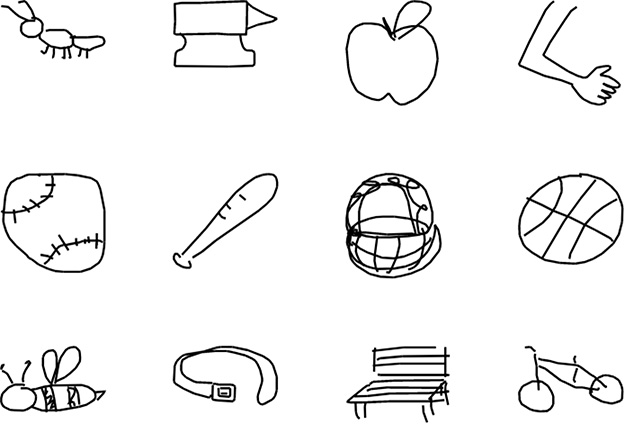
Figure 12.4 Example of sketches drawn by humans who have played the Quick, Draw! game. Baseballs, baskets, and bees—oh my!
5. If you have a lot of compute resources available to you (we’d recommend multiple GPUs), you could train a GAN on the data from all 345 sketch categories simultaneously. We haven’t tested this, so it really would be an adventure.
The GitHub repository of the Quick, Draw! game dataset can be accessed via bit.ly/QDrepository. The data are available in several formats there, including as raw and unmoderated images. In the interest of having relatively uniform data, we recommend using preprocessed data, which are centered and scaled doodles, among other more-technical adjustments. Specifically, for the simplicity of working with the data in Python, we recommend selecting the NumPy-formatted bitmaps of the preprocessed data.6
6. These particular data are available at bit.ly/QDdata for you to download.
We downloaded the apple.npy file, but you could pick any category that you desire for your own GAN. The contents of our Jupyter working directory are shown in Figure 12.5 with the data file stored here:
/deep-learning-illustrated/quickdraw_data/apples.npy

Figure 12.5 The directory structure inside the Docker container that is running Jupyter. We put our quickdraw_data directory (for storing Quick, Draw! NumPy bitmaps) at the same level as our notebooks directory (which contains all of the Jupyter notebooks we’ve been running in this book).
You’re welcome to store the data elsewhere, and you’re welcome to change the filename (especially if you downloaded a category other than apples); if you do, however, be mindful that you’ll need to update your data-loading code (coming up in Example 12.2) accordingly.
The first step, as you should be used to by now, is to load the package dependencies. For our Generative Adversarial Network notebook, these dependencies are provided in Example 12.1.7
7. Our GAN architecture is based on Rowel Atienza’s, which you can check out in GitHub via bit.ly/mnistGAN.
Example 12.1 Generative adversarial network dependencies
# for data input and output:
import numpy as np
import os

# for deep learning:
import keras
from keras.models import Model
from keras.layers import Input, Dense, Conv2D, Dropout
from keras.layers import BatchNormalization, Flatten
from keras.layers import Activation
from keras.layers import Reshape # new!
from keras.layers import Conv2DTranspose, UpSampling2D # new!
from keras.optimizers import RMSprop # new!

# for plotting:
import pandas as pd
from matplotlib import pyplot as plt
%matplotlib inline
All of these dependencies have popped up previously in this book except for three new layers and the RMSProp optimizer,8 which we’ll go over as we design our model architecture.
8. We introduced RMSProp in Chapter 9. Skip back to the section “Fancy Optimizers” if you’d like a refresher.
Okay, now back to loading the data. Assuming you set up your directory structure the same as ours and downloaded the apple.npy file, you can load these data in using the command in Example 12.2.
Example 12.2 Loading the Quick, Draw! data
input_images = "../quickdraw_data/apple.npy"
data = np.load(input_images)
Again, if your directory structure is different from ours or you selected a different category of NumPy images from the Quick, Draw! dataset, then you’ll need to amend the input_images path variable to your particular circumstance.
Running data.shape outputs the two dimensions of your training data. The first dimension is the number of images. At the time of this writing, the apples category had 145,000 images, but there are likely to be more by the time you’re reading this. The second dimension is the pixel count of each image. This value is 784, which should be familiar because—like the MNIST digits—these images have a 28×28-pixel shape.
Not only do these Quick, Draw! images have the same dimensions as the MNIST digits, but they are also represented as 8-bit integers, that is, integers ranging from 0 to 255. You can examine one—say, the 4,243rd image—by executing data[4242]. Because the data are still in a one-dimensional array, this doesn’t show you much. You should reformat the data as follows:
data = data/255
data = np.reshape(data,(data.shape[0],28,28,1))
img_w,img_h = data.shape[1:3]
Let’s examine this code line by line:
We divide by
255to scale our pixels to be in the range of 0 to 1, just as we did for the MNIST digits.9The first hidden layer of our discriminator network will consist of two-dimensional convolutional filters, so we convert the images from 1 × 784-pixel arrays to 28 × 28-pixel matrices. The NumPy
reshape()method does this for us. Note that the fourth dimension is1because the images are monochromatic; it would be3if the images were full-color.We store the image width (
img_w) and height (img_h) for use later.
9. See the footnote near Example 5.4 for an explanation as to why we scale in this way.
Figure 12.6 provides an example of what our reformatted data look like. We printed that example—a bitmap of the 4,243rd sketch from the apple category—by running this code:
plt.imshow(data[4242,:,:,0], cmap='Greys')

Figure 12.6 This example bitmap is the 4,243rd sketch from the apple category of the Quick, Draw! dataset.
The Discriminator Network
Our discriminator is a fairly straightforward convolutional network, involving the Conv2D layers detailed in Chapter 10 and the Model class introduced at the end of Chapter 11. See the code in Example 12.3.
Example 12.3 Discriminator model architecture
def build_discriminator(depth=64, p=0.4):

    # Define inputs
    image = Input((img_w,img_h,1))

    # Convolutional layers
    conv1 = Conv2D(depth*1, 5, strides=2,
                   padding='same', activation='relu')(image)
    conv1 = Dropout(p)(conv1)

    conv2 = Conv2D(depth*2, 5, strides=2,
               padding='same', activation='relu')(conv1)
    conv2 = Dropout(p)(conv2)

    conv3 = Conv2D(depth*4, 5, strides=2,
                   padding='same', activation='relu')(conv2)
    conv3 = Dropout(p)(conv3)

    conv4 = Conv2D(depth*8, 5, strides=1,
               padding='same', activation='relu')(conv3)
    conv4 = Flatten()(Dropout(p)(conv4))

    # Output layer
    prediction = Dense(1, activation='sigmoid')(conv4)

    # Model definition
    model = Model(inputs=image, outputs=prediction)

    return model
For the first time in this book, rather than create a model architecture directly we instead define a function (build_discriminator) that returns the constructed model object. Considering the schematic of this model in Figure 12.7 and the code in Example 12.3, let’s break down each piece of the model:
The input images are 28×28 pixels in size. This is passed to the input layer by the variables
img_wandimg_h.There are four hidden layers, and all of them are convolutional.
The number of convolutional filters per layer doubles layer-by-layer such that the first hidden layer has 64 convolutional filters (and therefore outputs an activation map with a depth of 64), whereas the fourth hidden layer has 512 convolutional filters (corresponding to an activation map with a depth of 512).10
The filter size is held constant at 5 × 5.11
The stride length for the first three convolutional layers is 2 × 2, which means that the activation map’s height and width are roughly halved by each of these layers (recall Equation 10.3). The stride length for the last convolutional layer is 1 × 1, so the activation map it outputs has the same height and width as the activation map input into it (4 × 4).
Dropout of 40 percent (
p=0.4) is applied to every convolutional layer.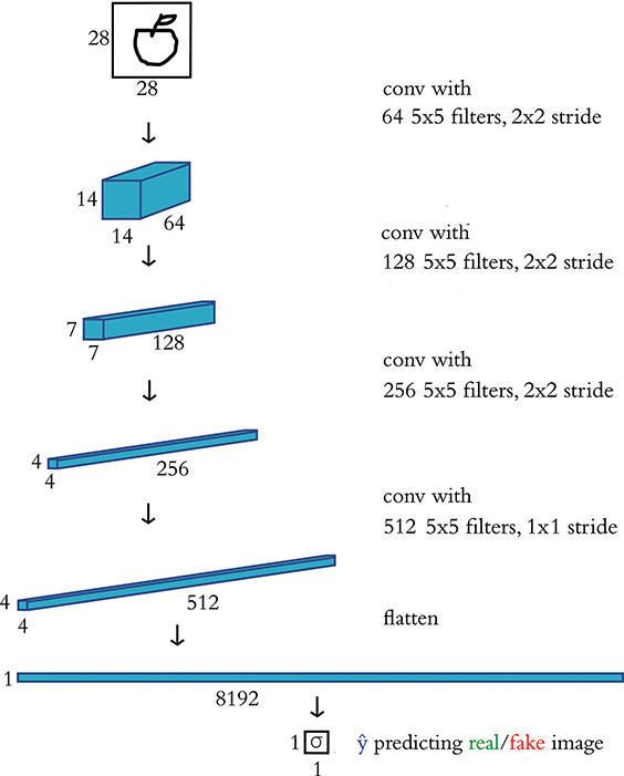
Figure 12.7 A schematic representation of our discriminator network for predicting whether an input image is real (in this case, a hand-drawn apple from the Quick, Draw! dataset) or fake (produced by an image generator)
We flatten the three-dimensional activation map from the final convolutional layer so that we can feed it into the dense output layer.
As with the film sentiment models in Chapter 11, discriminating real images from fakes is a binary classification task, so our (dense) output layer consists of a single sigmoid neuron.
10. More filters lead to more parameters and more model complexity, but also contribute to greater sharpness in the images the GANs produce. These values work well enough for this example.
11. We’ve largely used a filter size of 3 × 3 thus far in the book, although GANs can benefit from a slightly larger filter size, especially earlier in the network.
To build the discriminator, we call our build_discriminator function without any arguments:
discriminator = build_discriminator()
A summary of the model architecture can be output by calling the model’s summary method, which shows that the model has a total of 4.3 million parameters, most of which (76 percent) are associated with the final convolutional layer.
Example 12.4 provides code for compiling the discriminator.
Example 12.4 Compiling the discriminator network
discriminator.compile(loss='binary_crossentropy',
                      optimizer=RMSprop(lr=0.0008,
                                        decay=6e-8,
                                        clipvalue=1.0),
                      metrics=['accuracy'])
Let’s look at Example 12.4 line by line:
As in Chapter 11, we use the binary cross-entropy cost function because the discriminator is a binary classification model.
Introduced in Chapter 9, RMSprop is an alternative “fancy optimizer” to Adam.12
The decay rate (
decay, ρ) for the RMSprop optimizer is a hyperparameter described in Chapter 9.Finally,
clipvalueis a hyperparameter that prevents (i.e., clips) the gradient of learning (the partial-derivative relationship between cost and parameter values during stochastic gradient descent) from exceeding this value;clipvaluethereby explicitly limits exploding gradients (see Chapter 9). This particular value of1.0is common.
12. Ian Goodfellow and his colleagues published the first GAN paper in 2014. At the time, RMSProp was an optimizer already in vogue (the researchers Kingma and Ba published on Adam in 2014 as well, and it has become more popular in the years since). You might need to tune the hyperparameters a bit, but you could probably substitute RMSProp with Adam to similar effect.
The Generator Network
Although the CNN architecture of the discriminator network should largely look familiar, the generator network contains a number of aspects that you haven’t encountered previously in this book. The generator model is shown schematically in Figure 12.8.

Figure 12.8 A schematic representation of our generator network, which takes in noise (in this case, representing 32 latent-space dimensions) and outputs a 28×28-pixel image. After training as part of an adversarial network, these images should resemble images from the training dataset (in this case, hand-drawn apples).
We refer to the generator as a deCNN because it features de-convolutional layers (also known as convTranspose layers) that perform the opposite function of the typical convolutional layers you’ve encountered so far. Instead of detecting features and outputting an activation map of where the features occur in an image, de-convolutional layers take in an activation map and arrange the features spatially as outputs. An early step in the generative network reshapes the noise input (a one-dimensional vector) into a two-dimensional array that can be used by the de-convolutional layers. Through several layers of de-convolution, the generator converts the random noise inputs into fake images.
The code to build the generator model is in Example 12.5.
Example 12.5 Generator model architecture
z_dimensions = 32
def build_generator(latent_dim=z_dimensions,
                    depth=64, p=0.4):

    # Define inputs
    noise = Input((latent_dim,))

    # First dense layer
    dense1 = Dense(7*7*depth)(noise)
    dense1 = BatchNormalization(momentum=0.9)(dense1)
    dense1 = Activation(activation='relu')(dense1)
    dense1 = Reshape((7,7,depth))(dense1)
    dense1 = Dropout(p)(dense1)

    # De-Convolutional layers
    conv1 = UpSampling2D()(dense1)
    conv1 = Conv2DTranspose(int(depth/2),
                            kernel_size=5, padding='same',
                            activation=None,)(conv1)
    conv1 = BatchNormalization(momentum=0.9)(conv1)
    conv1 = Activation(activation='relu')(conv1)

    conv2 = UpSampling2D()(conv1)
    conv2 = Conv2DTranspose(int(depth/4),
                            kernel_size=5, padding='same',
                            activation=None,)(conv2)
    conv2 = BatchNormalization(momentum=0.9)(conv2)
    conv2 = Activation(activation='relu')(conv2)

    conv3 = Conv2DTranspose(int(depth/8),
                            kernel_size=5, padding='same',
                            activation=None,)(conv2)
    conv3 = BatchNormalization(momentum=0.9)(conv3)
    conv3 = Activation(activation='relu')(conv3)

    # Output layer
    image = Conv2D(1, kernel_size=5, padding='same',
                   activation='sigmoid')(conv3)

    # Model definition
    model = Model(inputs=noise, outputs=image)

    return model
Let’s go through the architecture in detail:
We specify the number of dimensions in the input noise vector (
z_dimensions) as 32. Configuring this hyperparameter follows the same advice we gave for selecting the number of dimensions in word-vector space in Chapter 11: A higher-dimensional noise vector has the capacity to store more information and thus can improve the quality of the GAN’s fake-image output; however, this comes at the cost of increased computational complexity. Generally, we recommend experimenting with varying this hyperparameter by multiples of 2.As with our discriminator model architecture (Example 12.3), we again opted to wrap our generator architecture within a function.
The input is the random noise array with a length corresponding to
latent_dim, which in this case is 32.The first hidden layer is a dense layer. This fully connected layer enables the latent-space input to be flexibly mapped to the spatial (de-convolutional) hidden layers that follow. The 32 input dimensions are mapped to 3,136 neurons in the dense layer, which outputs a one-dimensional array of activations. These activations are then reshaped into a 7×7×64 activation map. This dense layer is the only layer in the generator where dropout is applied.
The network has three de-convolutional layers (specified by
Conv2DTranspose). The first has 32 filters, and this number is halved successively in the remaining two layers.13 While the number of filters decreases, the size of the filters increases, thanks to the upsampling layers (UpSampling2D). Each time upsampling is applied (with its default parameters, as we use it here), both the height and the width of the activation map double.14 All three de-convolutional layers have the following:5×5
Stride of 1 × 1 (the default)
Padding set to
sameto maintain the dimensions of the activation maps after de-convolutionReLU activation functions
Batch normalization applied (to promote regularization)
The output layer is a convolutional layer that collapses the 28×28×8 activation maps into a single 28×28×1 image. The sigmoid activation function in this last step ensures that the pixel values range from
0to1, just like the data from real images that we feed into the discriminator separately.
13. As with convolutional layers, the number of filters in the layer corresponds to the number of slices (the depth) of the activation map the layer outputs.
14. This makes upsampling roughly the inverse of pooling.
Exactly as we did with the discriminator network, we call the build_generator function without supplying any arguments to build the generator:
generator = build_generator()
Calling the model’s summary method shows that the generator has only 177,000 trainable parameters—a mere 4 percent of the number of parameters in the discriminator.
The Adversarial Network
Combining the training processes from Figures 12.2 and 12.3, we arrive at the outline in Figure 12.9. By executing the code examples so far in this chapter, we have accomplished the following:
With respect to discriminator training (Figure 12.2), we’ve constructed our discriminator network and compiled it: It’s ready to be trained on real and fake images so that it can learn how to distinguish between these two classes.
With respect to generator training (Figure 12.3), we’ve constructed our generator network, but it needs to be compiled as part of the larger adversarial network in order to be ready for training.
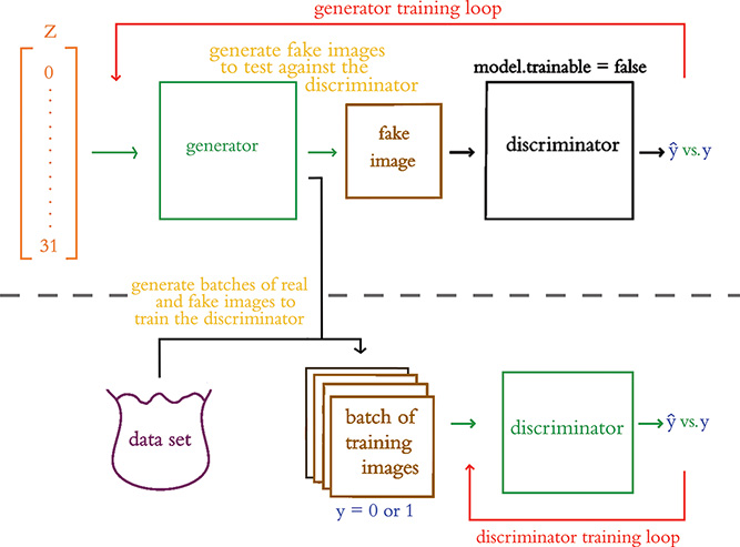
Figure 12.9 Shown here is a summary of the whole adversarial network. The horizontal dashes visually separate generator training from discriminator training. Green lines indicate trainable paths, whereas inference-only paths are in black. The red arrows above and below indicate the path of the backpropagation step during the respective training processes.
To combine our generator and discriminator networks to build an adversarial network, we use the code in Example 12.6.
Example 12.6 Adversarial model architecture
z = Input(shape=(z_dimensions,))
img = generator(z)
discriminator.trainable = False
pred = discriminator(img)
adversarial_model = Model(z, pred)
Let’s break this code down:
We use
Input()to define the model’s inputz, which will be an array of random noise of length 32.Passing
zintogeneratorreturns a 28×28 image output that we callimg.For the purposes of generator training, the parameters of our discriminator network must be frozen (see Figure 12.3), so we set the discriminator’s
trainableattribute toFalse.We pass the fake
imginto the frozendiscriminatornetwork, which outputs a prediction (pred) as to whether the image is real or fake.Finally, using the Keras functional API’s
Modelclass, we construct the adversarial model. By indicating that the adversarial model’s input iszand its output ispred, the functional API determines that the adversarial network consists of the generator passingimginto the frozen discriminator.
To compile the adversarial network, we use the code in Example 12.7.
Example 12.7 Compiling the adversarial network
adversarial_model.compile(loss='binary_crossentropy',
                          optimizer=RMSprop(lr=0.0004,
                                            decay=3e-8,
                                            clipvalue=1.0),
                          metrics=['accuracy'])
The arguments to the compile() method are the same as those we used for the discriminator network (see Example 12.4), except that the optimizer’s learning rate and decay have been halved. There’s a somewhat delicate balance to be struck between the rate at which the discriminator and the generator learn in order for the GAN to produce compelling fake images. If you were to adjust the optimizer hyperparameters of the discriminator model when compiling it, then you might find that you’d also need to adjust them for the adversarial model in order to produce satisfactory image outputs.
![]()
GAN Training
To train our GAN, we call the (cleverly titled) function train, which is provided in Example 12.8.
Example 12.8 GAN training
def train(epochs=2000, batch=128, z_dim=z_dimensions):

    d_metrics = []
    a_metrics = []

    running_d_loss = 0
    running_d_acc = 0
    running_a_loss = 0
    running_a_acc = 0

    for i in range(epochs):

        # sample real images:
        real_imgs = np.reshape(
            data[np.random.choice(data.shape[0],
                                  batch,
                                  replace=False)],
            (batch,28,28,1))

       # generate fake images:
       fake_imgs = generator.predict(
           np.random.uniform(-1.0, 1.0,
                             size=[batch, z_dim]))

       # concatenate images as discriminator inputs:
       x = np.concatenate((real_imgs,fake_imgs))

       # assign y labels for discriminator:
       y = np.ones([2*batch,1])
       y[batch:,:] = 0

       # train discriminator:
       d_metrics.append(
           discriminator.train_on_batch(x,y)
       )
       running_d_loss += d_metrics[-1][0]
       running_d_acc += d_metrics[-1][1]

       # adversarial net's noise input and "real" y:
       noise = np.random.uniform(-1.0, 1.0,
                                 size=[batch, z_dim])
       y = np.ones([batch,1])

       # train adversarial net:
       a_metrics.append(
          adversarial_model.train_on_batch(noise,y)
       )
       running_a_loss += a_metrics[-1][0]
       running_a_acc += a_metrics[-1][1]

       # periodically print progress & fake images:
       if (i+1)%100 == 0:

           print('Epoch #{}'.format(i))
           log_mesg = "%d: [D loss: %f, acc: %f]" %
           (i, running_d_loss/i, running_d_acc/i)
           log_mesg = "%s [A loss: %f, acc: %f]" %
           (log_mesg, running_a_loss/i, running_a_acc/i)
           print(log_mesg)

           noise = np.random.uniform(-1.0, 1.0,
                                     size=[16, z_dim])
           gen_imgs = generator.predict(noise)

           plt.figure(figsize=(5,5))

           for k in range(gen_imgs.shape[0]):
               plt.subplot(4, 4, k+1)
               plt.imshow(gen_imgs[k, :, :, 0],
                          cmap='gray')
               plt.axis('off')

           plt.tight_layout()
           plt.show()

     return a_metrics, d_metrics

# train the GAN:
a_metrics_complete, d_metrics_complete = train()
This is the largest single chunk of code in the book, so from top to bottom, let’s dissect it to understand it better:
The two empty lists (e.g.,
d_metrics) and the four variables set to0(e.g.,running_d_loss) are for tracking loss and accuracy metrics for the discriminator (d) and adversarial (a) networks as they train.We use the
forloop to train for however manyepochswe’d like. Note that while the term epoch is commonly used by GAN developers for this loop, it would be more accurate to call it a batch: During each iteration of theforloop, we will sample only128apple sketches from our dataset of hundreds of thousands of such sketches.Within each epoch, we alternate between discriminator training and generator training.
To train the discriminator (as depicted in Figure 12.2), we:
Sample a batch of 128 real images.
Generate 128 fake images by creating noise vectors (
z, sampled uniformly over the range [–1:0, 1:0]) and passing them into the generator model’spredictmethod. Note that by using thepredictmethod, the generator is only performing inference; it is generating images without updating any of its parameters.Concatenate the real and fake images into a single variable
x, which will serve as the input into our discriminator.Create an array,
y, to label the images as real (y = 1) or fake (y = 0) so that they can be used to train the discriminator.To train the
discriminator, we pass our inputsxand labelsyinto the model’strain_on_batchmethod.After each round of training, the training loss and accuracy metrics are appended to the
d_metricslist.
To train the generator (as in Figure 12.3), we:
Pass random noise vectors (stored in a variable called
noise) as inputs as well as an array (y) of all-real labels (i.e., y = 1) into thetrain_on_batchmethod of the adversarial model.The generator component of the adversarial model converts the
noiseinputs into fake images, which are automatically passed as inputs into the discriminator component of the adversarial model.Because the discriminator’s parameters are frozen during adversarial model training, the discriminator will simply tell us whether it thinks the incoming images are real or fake. Even though the generator outputs fakes, they are labeled as real (y = 1) and the cross-entropy cost is used during backpropagation to update the weights of the generator model. By minimizing this cost, the generator should learn to produce fake images that the discriminator erroneously classifies as real.
After each round of training, the adversarial loss and accuracy metrics are appended to the
a_metricslist.
After every 100 epochs we:
Print the epoch that we are in.
Print a log message that includes the discriminator and adversarial models’ running loss and accuracy metrics.
Randomly sample 16 noise vectors and use the generator’s
predictmethod to generate fake images, which are stored ingen_imgs.Plot the 16 fake images in a 4×4 grid so that we can monitor the quality of the generator’s images during training.
At the conclusion of the
trainfunction, we return the lists of adversarial model and discriminator model metrics (a_metricsandd_metrics, respectively).Finally, we call the
trainfunction, saving the metrics into thea_metrics_completeandd_metrics_completevariables as training progresses.
After 100 rounds (epochs) of training (see Figure 12.10), our GAN’s fake images appear to have some vague sketch-like structure, but we can’t yet discern apples in them. After 200 rounds, however (see Figure 12.11), the images do begin to have a loose appley-ness to them. Over several hundred more rounds of training, the GAN begins to produce some compelling forgeries of apple sketches (Figure 12.12). And, after 2,000 rounds, our GAN output the “machine art” demo images that we provided way back at the end of Chapter 3 (Figure 3.9).

Figure 12.10 Fake apple sketches generated after 100 epochs of training our GAN
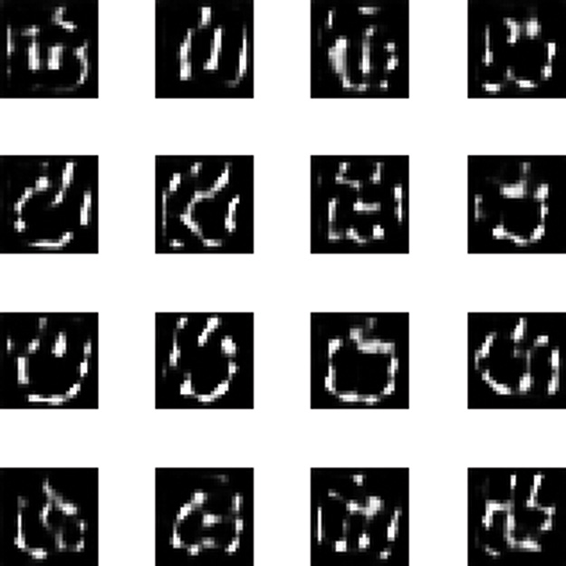
Figure 12.11 Fake apple sketches after 200 epochs of training our GAN

Figure 12.12 Fake apple sketches after 1,000 epochs of training our GAN
To wrap up our Generative Adversarial Network notebook, we ran the code in Examples 12.9 and 12.10 to create plots of our GAN’s training loss (Figure 12.13) and training accuracy (Figure 12.14). These show that the adversarial model’s loss declined as the quality of the apple-sketch forgeries improved; that is what we’d expect because this model’s loss is associated with fake images being misclassified as real ones by the discriminator network, and you can see from Figures 12.10, 12.11, and 12.12 that, the longer we trained, the increasingly real the fakes appeared. As the generator component of the adversarial model began to produce higher-quality fakes, the discriminator’s task of discerning real apple sketches from fake ones became more difficult, and so its loss generally rose over the first 300 epochs. From the ~300th epoch onward, the discriminator modestly improved at its binary classification task, corresponding to a gentle decrease in its training loss and an increase in its training accuracy.

Figure 12.13 GAN training loss over epochs
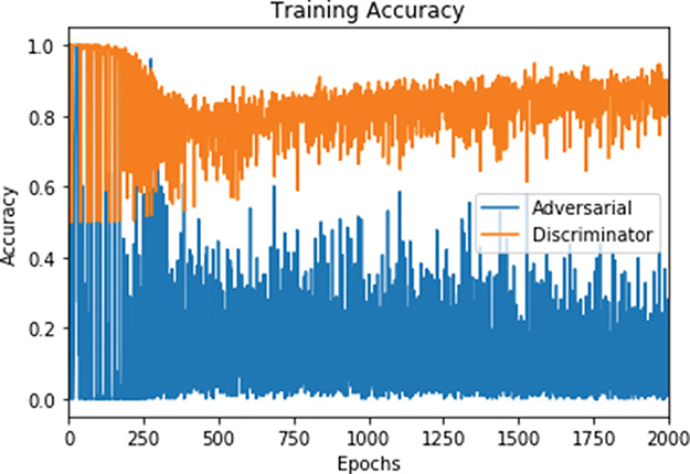
Figure 12.14 GAN training accuracy over epochs
Example 12.9 Plotting our GAN training loss
ax = pd.DataFrame(
     {
        'Adversarial': [metric[0] for metric in a_metrics_complete],
        'Discriminator': [metric[0] for metric in d_metrics_complete],
     }
).plot(title='Training Loss', logy=True)
ax.set_xlabel("Epochs")
ax.set_ylabel("Loss")
Example 12.10 Plotting our GAN training accuracy
ax = pd.DataFrame(
     {
        'Adversarial': [metric[1] for metric in a_metrics_complete],
        'Discriminator': [metric[1] for metric in d_metrics_complete],
     }
).plot(title='Training Accuracy')
ax.set_xlabel("Epochs")
ax.set_ylabel("Accuracy")
Summary
In this chapter, we covered the essential theory of GANs, including a couple of new layer types (de-convolution and upsampling). We constructed discriminator and generator networks and then combined them to form an adversarial network. Through alternately training a discriminator model and the generator component of the adversarial model, the GAN learned how to create novel “sketches” of apples.
Key Concepts
Here are the essential foundational concepts thus far. New terms from the current chapter are highlighted in purple.
parameters:
weight w
bias b
activation a
artificial neurons:
sigmoid
tanh
ReLU
linear
input layer
hidden layer
output layer
layer types:
dense (fully connected)
softmax
convolutional
de-convolutional
max-pooling
upsampling
flatten
embedding
RNN
(bidirectional-)LSTM
concatenate
cost (loss) functions:
quadratic (mean squared error)
cross-entropy
forward propagation
backpropagation
unstable (especially vanishing) gradients
Glorot weight initialization
batch normalization
dropout
optimizers:
stochastic gradient descent
Adam
optimizer hyperparameters:
learning rate η
batch size
word2vec
GAN components:
discriminator network
generator network
adversarial network