1
Essential Modeling Heuristics

1.1 Introduction

In Structured Development for Real-Time Systems, Volume 1, Chapter 4 (Modeling Heuristics), we defined an essential model as one that describes those things that a system must do to be successful, regardless of the technology chosen to implement it. In Chapters 6 through 13 of Volume 1, we introduced a modeling notation, which, as we shall demonstrate, is adequate to express the details of an essential model rigorously.

Unfortunately, neither an understanding of the characteristics of an essential model, nor a knowledge of the modeling notation, guarantees that a successful model can actually be built. Some guidelines – some modeling heuristics – are needed. These heuristics must be specific enough to provide detailed guidance to the model-builder yet general enough to cover the spectrum of situations in which an essential model must be built.

In this chapter we will introduce three powerful guidelines for essential model building: environment-based modeling, subject-matter-centered modeling, and minimum-complexity representation. Before discussing these in detail, let’s look at a commonly used heuristic for modeling requirements and examine its inadequacies.

1.2 Problems with Functional Decomposition

Functional decomposition is a specific application of the idea of top-down development discussed in Volume 1, Chapter 4. The developer begins by envisioning a system, or part of a system, as a single function (in other words, as a transformation of inputs into outputs). The system is then decomposed into a small set of sub-functions equivalent to the original function, and the interfaces between the subfunc-tions are identified. Each subfunction then becomes the starting point for a further decomposition into sub-subfunctions and identification of lower-level interfaces. The process continues until the lowest level of functions is simple enough to be specified in detail.

As an example, consider the specification of a control system for a picture-taking satellite. The modeler using functional decomposition might conceive of the overall function of the system as “Manage optical data collection.” This function might then be decomposed into “Manage data transmission,” “Manage data storage,” “Manage mechanical equipment control,” and other major subfunctions. “Manage data transmission” might be further decomposed into “Manage message input” and “Manage message output,” and so on. Figure 1.1 illustrates this process schematically.

Figure 1.1 Illustration of Functional Decomposition.

Functional decomposition has an attractive pedigree: it was one of the earliest development techniques, and it neatly matches top-down presentation techniques such as the notation described in Chapter 12 of Volume 1 (Organizing the Model). Nevertheless, there are major problems with this approach. First, Heitmeyer and McLean [1] argue that any statement of requirements arrived at by decomposition is implementation-dependent, since a more-or-less arbitrary choice among a set of possible decompositions has been made. An arbitrary choice of subsystems boundaries imposed by decomposition may thus prevent an implementer from using perfectly adequate algorithms that happen to be inconsistent with these boundaries.

Second, it has been our experience that the technique often does not produce good partitionings. Although criteria exist for evaluating alternate decompositions on the basis of interface complexity (Parnas [2] and DeMarco [3]), this is an after-the-fact approach that eliminates possible solutions only after the work is put in to create them. Functional decomposition does nothing to guide the developer to a partitioning with minimum interfaces. The technique thus invites “analysis paralysis,” in which endless discussions of the merits of various top-level partitionings of the model preclude progress toward understanding of the specifics.

These problems, taken together, cause us to regard functional decomposition as being of very limited value.

We feel that the shortcomings of functional decomposition arise from its failure to make explicit use of all the information available to the developer at requirements definition. Specifically, functional decomposition fails to focus on the environment in which the system to be built must operate.

This leads to our next topic, the application of environment-based modeling to the building of an essential model.

1.3 Environment-Based Modeling

To be sure that all the relevant information about the environment is captured in the essential model, it is beneficial actually to incorporate a model of the environment into the essential model. Modeling the environment provides a framework that is an alternative to functional decomposition.

The most important task in developing the environmental model is to specify the events to which the system must respond. This specification is the basis for the creation of a behavioral model, using an elaboration of a technique developed by McMenamin and Palmer [4].

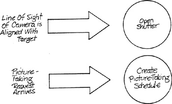
Let’s recall the picture-taking satellite example used to illustrate functional decomposition. Instead of attempting to identify subfunctions, sub-subfunctions, and so on, environment-based modeling would proceed by identifying events that require some system response. Possible events are “Line of sight of camera is aligned with target” and “Picture-taking request is made.” The behavioral model is then constructed by determining acceptable responses to the events, as illustrated in Figure 1.2.

Figure 1.2 Illustration of Environment-Based Modeling.

Although the behavioral model is a functional model (that is, it consists of a collection of transformations of inputs into outputs), it is derived not through decomposition but by a mapping of elements from the system’s environment into the model. Like the result of functional decomposition, the behavioral model can be represented by a leveled set of transformation schemas. In this case, the event responses would be aggregated into higher-level subsystems.

The event modeler carries out the mapping between the environmental and behavioral models by thinking of a system as a stimulus-response mechanism, which accomplishes a specific purpose by responding to events that occur in its environment. The identification of the events – the elemental stimuli that elicit a response from the system – provides a natural level of detail for a system description. The behavioral model has a point-by-point correspondence to identifiable parts of the environment in which the system will operate. It therefore has a low-level structure derived directly from the structure of the problem and should not bias the developer toward non-optimal solutions. In contrast to functional decomposition, this procedure may be thought of as “outside-in” rather than “top-down” modeling.

Although focusing on the system environment is useful, not all environmental elements are of equal relevance. Before examining the second major essential-modeling heuristic, subject-matter-centered modeling, let’s look at a classification scheme for these elements.

1.4 Components of the Total System

We focus in this book on systems that will ultimately involve building or adapting computer hardware and software to do the work described by the model. Systems of this type used in manufacturing, aerospace, and similar technological environments are called embedded systems. They are part of, and contribute to, systems that employ technology other than computer technology and whose primary purpose is not computation. An air traffic control system, for example, contains radars, radio transmitters, and radio receivers in addition to computers. Its purpose is to get aircraft safely into and out of some defined airspace: The computations performed by the computers within such a system, while important, are completely subordinate to the purpose of the larger system.

Alford [5] has proposed a characterization of the larger systems of which embedded systems are a part. Such systems have a perception space and an action space as illustrated by Figure 1.3. Objects (vehicles, people, and so on) enter the perception space of the system, are perceived by it, are acted upon, and finally leave the action space of the system. Some examples are given in Table 1.1

Figure 1.3 Perception-Action View of an Air Traffic Control System.

Table 1.1.

This characterization can easily be extended to traditional business systems: a savings account customer enters a bank, is identified by account number, is given some amount of money from his or her account, and leaves the bank.

In addition to the perception/action space objects, Alford identifies five components of systems matching his characterization: sensors, actors, computers, communication links, and people. We will use a slightly different scheme, lumping people and computers together and identifying the components as sensors, actors, communication links, and processors. (A single device sometimes serves as both a sensor and an actor.) To continue with the air traffic control example, the sensors would be the radar units, the actors would be the equipment that transmitted messages to the aircraft crew, and the communications links would be the data transmission lines, display terminals, and other equipment that passes information and control among radars, transmitters, computers, and air traffic control staff.

Let’s now use this classification to describe the application of subject-matter-centered modeling.

1.5 Subject-Matter-Centered Modeling

Consider the components of the total system grouped and listed as perception/action space objects, sensors/actors, communication links, and processors. An ordering has been defined from maximum to minimum subject-matter constraint. The perception/action space objects are, by definition, completely constrained by the subject matter. Changing the nature of these objects changes the nature of the system. A system that perceives and acts on parts on an assembly line has quite a different subject matter from one that perceives and acts on bank customers. Sensors and actors are somewhat constrained by the system’s subject matter, but typically have some flexibility in their selection. A satellite cannot use a thermocouple or a pH sensor to detect troop movements on the ground, but it can use any of a wide variety of electromagnetic radiation sensors. Communications links are in turn somewhat constrained by the nature of the sensors and actors that they tie to the system’s processors, but the subject-matter-specificity is considerably less. Processors, of course, are by definition subject-matter non-specific, and are thus at the low end of the constraint scale.

The significance of the constraint scale is that only the portions of the (actual or anticipated) environment that are subject-matter-specific should influence the structure of the behavioral model. Let’s use as an example the type of keyboard illustrated in Figure 1.4. Depression of a key causes contact between one of the input (read) lines and one of the output (write) lines. The keyboard is operated by periodically energizing the write lines one at a time, then checking the read lines for non-zero voltage. For example, a non-zero voltage on read line 2 while write line 0 is energized means that the ‘7’ key is being depressed.

Figure 1.4 Keyboard Configuration.

Consider an embedded system that will act as a keyboard device handler. The keyboard is an object in the perception/action space of this system. The values of the read lines are perceived, and the write lines are acted on. It is reasonable to expect functions within the essential model for this device handler to have names drawn from the perception/action space, such as “Energize write line” and “Store read line value.”

Now consider a system that operates in a chemical plant to monitor the parameters of a chemical reaction. A system of this kind could be implemented so that a technician reads a dial on the reaction vessel and keys in the reading. Although the keyboard of Figure 1.4 might be used in this system, it plays the role of a communications link rather than of a perception/action space object. An essential model for this type of system would contain functions like “Record pH value,” referring to the chemical reaction that is the perception/action space object, but should not contain functions referring to the keyboard technology. An implementation change for this system, such as replacing the keyboard by a direct link to the reaction vessel, should not affect the essential model.

1.6 Minimum-Complexity Representation

Since any system must respond to its environment, the behavioral model of the system must contain some representation of the relevant portions of the environment. In the case of an air-traffic control system, one can ask about the system’s representation of an aircraft, of the boundaries of the air space, and so on.

The heuristic of minimum-complexity representation states that the simplest representation that adequately models a situation should be chosen. Traditional process-oriented models of business systems have represented the system environment in terms of values of stored data elements. The data transformations in Figure 1.5, for example, are organized around the Inventory Items store. Each entry within the store represents one of the inventory items in the system’s environment, including the Quantity Available and the Item ID. The system is represented entirely in terms of data transformations, data flows, and data stores, which is inevitable since these are the only notational elements available in the traditional process model. However, it is reasonable to ask whether the extended notation of the transformation schema is useful for describing this system.

Figure 1.5 Representing the Environment in Stored Data.

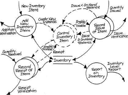
To explore this, let’s look at a state-transition diagram for a particular inventory item (Figure 1.6). The item isn’t in a defined state until it has been added to the system; thereafter it moves between Out of Stock and Available, depending on the pattern of receipts and issues. One could represent the system from Figure 1.5 by incorporating a set of control transformations, one for each existing type of item, each with an associated state diagram identical to Figure 1.6. Each control transformation would manage its own Record Receipt of Item and Record Issue of Item data transformations. The resulting transformation schema is shown in Figure 1.7. Although the notation is quite different, Figure 1.7 has many conceptual similarities to the Jackson System Design method. Jackson and Cameron [6] routinely represent multiple instances of objects in the system’s environment by multiple transformations, which they call sequential processes. Each instance of the transformation remembers the status of a particular instance of the object in the system’s environment. The specification for the transformation must define the possible values for the status of the object and the permissible sequences of statuses. Contrast this representation to that shown in Figure 1.5. In this model, data about multiple instances of an object in the environment may exist in the store, and the change in status from Available to Out of Stock is managed jointly by Record Receipt of Item and Record Issue of Item. The coordination required between these two transformations requires only shared data access and is simpler than the stored data and control connections illustrated in Figure 1.7. We therefore argue that Figure 1.5 is preferable because of its simplicity and clarity.

Figure 1.6 State Transition Diagram for Inventory Data.

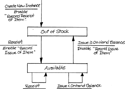
Figure 1.7 Inventory System with Control Transformations.

Let’s now turn the situation around and ask whether situations that we have been modeling with control transformations can be represented more simply in data transformation terms. Figure 1.8 illustrates a model of the Cruise Control System (Appendix A) in which each input is handled by a separate data transformation as was done in Figure 1.5, and in which the Status data store links the transformations and represents the state of the speed control mechanism. The possible values of status are Stopped, Maintaining Speed, Interrupted by Braking, and Resuming Speed. This picture has an appealing simplicity. Unfortunately, the Status data store does not show a true time-delayed connection among the processes as does the Inventory Items store in Figure 1.5. In fact, any change of status will immediately impact the behavior of Control Throttle. The model doesn’t clearly describe the causal connections between the inputs and the resulting behaviors of the system. Although simple, the representation is not adequate.

Figure 1.8 Data-Transformation-Only Version of Cruise Control.

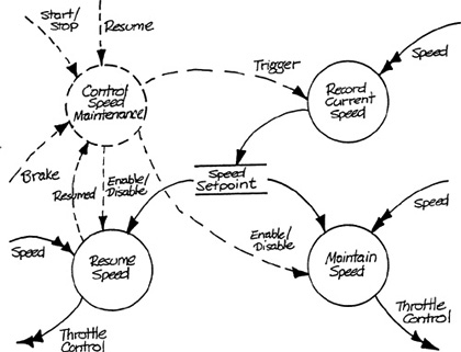
In Figure 1.9, we have used a control transformation to model the interaction between the event flows and the operation of the data transformations. The state transition diagram associated with the Control Speed Maintenance transformation specifies the interaction in discrete terms.

To summarize, one can represent something in a system’s environment (sensor/actor technology, or objects in the perception/action space) in either stored data or state transition terms. The stored data representation is characterized by separate data transformations assigned to separate inputs. Connections among transformations are non-causal, time-delayed storage links. The state of the object in the environment is expressed by stored data values. Multiple instances of the object in the environment are expressed by tags, identifying the instance, attached to input flows and to the stored data.

The state transition representation is characterized by a control transformation accepting multiple control inputs and driving multiple data transformations. Connections between transformations are immediate, causal event flow linkages. The state of the object in the environment is represented by a state associated with the control transformation. Multiple instances of the object in the environment are represented by multiple control transformations (multiple sets of states), each controlling individual sets of data transformations. The principle of minimum-complexity representation guides the choice of which representation to use in a particular case.

Figure 1.9 Control Transformation Added to Cruise Control Schema.

1.7 Summary

Essential modeling is fundamentally concerned with the issue of the subject matter of the system and deliberately defers implementation issues. In this chapter we have laid out heuristics for essential modeling that focus on the environment as a basis for constructing a model of the behavior of a system. To clarify the influence of the environment on an embedded system we have identified the roles played by the components of the total system in relation to their roles in an embedded system. Finally, we discussed two ways in which portions of the system can be represented in the essential model and conditions under which each can be the simplest representation of a system’s requirements.

Chapter 1: References

1. C.L. Heitmeyer and J.D. McLean, “Abstract Requirements Specification: A New Approach and Its Application,” IEEE Transactions on Software Engineering, Volume SE-9. No. 5, Sept. 1983, pp. 580-589.

2. D. Parnas, “On the Criteria to Be Used in Decomposing Systems into Modules.” Communications of the ACM, Vol. 5, No. 12 (December 1972), pp. 1053-58.

3. T. DeMarco, Structured Analysis and System Specification. New York: Yourdon Press, 1978.

4. S. McMenamin and J. Palmer, Essential Systems Analysis. New York: Yourdon Press, 1984.

5. M.W. Alford. “An Integrated Data/Control Flow Specification Technique” Paper Presented at the Rocky Mountain Institute for Software Engineering, Aspen, July 1984.

6. M. Jackson and J. Cameron, A Tutorial on JSD. London: Michael Jackson Associates, 1984.